10-100 TeV cosmic ray anisotropy measured at Baksan EAS ”Carpet” array

Abstract

Preliminary results of one year anisotropy measurement in the energy range $10^{13}-10^{14}$ eV as a function of energy are presented. The results are compared for two methods of data analysis: the standard one with meteo correction approach in use and another one so-called ”East minus West” method. Amplitudes and phases of anisotropy for three median energies E = 25 TeV, E = 75 TeV and E = 120 TeV are reported. Brief consideration of amplitude-phase dependence of anisotropy on energy is expounded.

1 Introduction

Experimental results on anisotropy of primary cosmic ray flux give important information for further theoretical study of the origin and propagation problems in cosmic ray physics. Together with numerical characteristics of anisotropy - amplitude and phase - the energy dependence of these characteristic gives additional information for better understanding of the above mentioned problems. Energy range of primary cosmic rays under anisotropy investigation is extremely wide - from $\sim$ 100 GeV up to $10^{5}$ TeV and higher. At 1 - 10 TeV range the measurements are carried out with detectors of Cerenkov emission of Extensive Air Showers or underground muon telescopes (Nagoya, Baksan Underground Scintillation Telescope; MACRO and others). Then, at 100-10000 TeV range, the EAS-TOP and CASCADE results are well known. And finally for $10^{17}$ eV and above anisotropy is studied with giant EAS installations such as Yakutsk, AGASA and Auger. One can find review of anisotropy results in [1] and bibliography in [1, 2, 3]. Some results of cosmic ray anisotropy studies with a Small Air Shower (SAS) arrays (E $\sim$ 10 TeV) in Northern hemisphere were published at seventieth-eightieth [4, 5, 6, 7, 8]. Amplitude and phase of anisotropy were derived from Fourier analysis of counting rate along the Right Ascension coordinate, without record of SAS arrival direction. The main results of those studies were: 1). Compton-Getting effect due to revolution of the Earth around the Sun in accordance with theoretical prediction [9] was observed, 2). Sidereal anisotropy with amplitude $\sim 0.06\%$ and phase $\sim$ 1 hour RA was measured with high statistical accuracy. When there are numerous results for E $<$ 10 TeV and E $>$ 100 TeV, the 10-100 TeV range is up to now slightly studied. Lack of experimental results at this energy range gives no possibility to arrive at clear conclusion about dependence of amplitude and phase of anisotropy on energy. At 2007, after some modernization of Baksan EAS installation, we resumed the measurement of anisotropy of SAS in the range 10-100 TeV with registration of arrival directions on celestial sphere. Below we report result of one year registration.

2 Experimental set-up and Energy Response

Central part of Baksan SAS array - ”Carpet” - consists of 400 liquid scintillation detectors, arranged in horizontal continuous square geometry - Fig.1. Dimension of the detector is 70x70x30 cm³. There are four outside huts (OH) on square diagonals at distance 30 m from the center of Carpet. Each hut contains 18 (3x6)detectors. The Carpet is divided into 25 square modules, each module = 16 detectors. Twenty nine (25 modules + 4 OH) sum anode pulses (each pulse is a sum of anode pulses of individual detectors of module) are registered with ADC, TDC and with multiple logic unit designed to produce the SAS triggers. Individual (each of 29) logic pulse is generated if corresponding sum anode pulse exceeds level corresponding to energy deposition of 0.5 relativistic particle. Energy deposition corresponding to 1 r.p. is equal 50 MeV. Multiplicity of individual logic signals together with anode amplitudes are the measure of power of SAS, following the primary particle energy.Arrival direction of SAS is calculated using the relative times from TDC channels. In the present analysis we have used three sorts of triggers:4-fold coincidence of corner modules 4CM, 4-fold coincidence of outside huts 4OH, 8-fold coincidence 4CM+4OH. Counting rate of coincidences: F(4CM)=1.39 Hz, F(4OH)=1.50 Hz, F(4CM+4OH)=0.72 Hz. Angular resolution: R(4CM)=$10^{o}$, R(4OH)=$3.5^{o}$, R(4CM+4OH)=$3.0^{o}$.One year data set was processed, only full days were included in analysis,useful time after ”noise” cuts and elimination of ”bad” days = $75\%$.Energy response for three sorts of trigger was evaluated by Monte Carlo simulations, made on the basis of CORSIKA codes (v. 6012, HDPM and Gheisha models). Vertical proton flux (with differential spectrum $\gamma$ = - 2.7) uniformly distributed over the circle area with r = 60 m was used in simulation. The roof of thickness 34 $g/cm^{2}$above the Carpet was taken into account. Evaluated median energies for three sorts of trigger are: E (4CM) = 25 TeV, E (4OH) = 75 TeV, E (4CM+4OH) = 120 TeV.

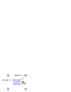
Figure 1: Plan of the Baksan SAS array.

3 Processing and analysis of experimental information.

Fourier analysis of resulting day waves in solar, sidereal and antisidereal time was done to find amplitudes and phases of the 1st and 2nd harmonics. Resulting day waves were obtained by two methods with posterior comparison of methods’ efficiency: a) traditional approach with meteo correction, b) differential method ”East minus West”. The following considerations were used as efficiency criteria: 1) Phase of the first solar harmonic must be close to 6 hours of Local Solar Time (Compton-Getting effect), and amplitude to be close to 0.034 for our geographic latitude. 2) Absence of statistically significant antisidereal wave. It means the absence of annual modulation of solar day wave. Otherwise the false sidereal wave inevitably arises as one of two side frequencies - sidereal and antisidereal.

3.1 Traditional approach

Counting rate in cosmic ray variation experiments depends essentially on variations of meteorological factors - atmosphere pressure and temperature. Hence, one need to exclude meteo induced variations to get pure initial variations of counting rate. Meteorological coefficients for three sorts of trigger were derived from multiple regression analysis. Amplitudes and phases of 1st harmonics after meteo correction are presented in Table 1. All 2nd harmonic amplitudes are inside statistics. It is necessary to note that comparatively large statistical error arises from short enough data set - only one year of registration. And nevertheless, phases of solar waves are in good coincidence with expected one from Compton-Getting effect - all three are close to 6 hour of Local Solar Time. At the same time extremely large ($>5\sigma$) amplitude of 75 TeV antisidereal wave gives rise to assume that meteo correction procedure by itself doesn’t guarantee total expulsion of extraneous variations. This fact arouses doubts about sidereal time result.

Table 1: Amplitudes and phases of 1st harmonic after meteo correction.The amplitude errors shown in Table1 and Table2 are statistical ones.

wave	Solar	Sidereal	Antisidereal
1st harmonic
25 TeV amplitude, $\%$	$0.025\pm 0.025$	$0.065\pm 0.025$	$0.064\pm 0.025$
phase, h	$6.4\pm 2.3$	$23.5\pm 1.4$	$19.1\pm 1.4$
75 TeV amplitude, $\%$	$0.050\pm 0.024$	$0.088\pm 0.024$	$0.122\pm 0.024$
phase, h	$7.5\pm 1.7$	$19.6\pm 1.0$	$1.2\pm 0.7$
120 TeV amplitude, $\%$	$0.047\pm 0.035$	$0.059\pm 0.035$	$0.087\pm 0.035$
phase, h	$6.8\pm 2.2$	$21.1\pm 1.7$	$22.4\pm 1.5$

3.2 East minus West method.

When studying anisotropy we come across not only with variations induced by meteo factors but also with apparatus instabilities. To remove them totally or simply to take into account their effect is not so easy task. Wit way to solve the problem is the ’East minus West” method mentioned for the first time in [10]. The method is based on the assumption that as meteo factors so apparatus instabilities produce equal variations in counting rates of showers arriving from East and West directions. Hence the difference between East-ward and West-ward counting rates can eliminate the uncontrolled and spurious variations. Sequence of differences of counting rates from two directions calculated during the day for each fixed time interval (20-min in our case) results in differential day wave.Then integration of resulting (sum of all days) differential wave results in primordial day wave characterized by amplitude and phase. Amplitudes and phases of 1st harmonics resulting from East-West method are presented in Table 2.

Table 2: Amplitudes and phases of 1st harmonic after East minus West method.

wave	Solar	Sidereal	Antisidereal
1st harmonic
25 TeV amplitude, $\%$	$0.046\pm 0.025$	$0.060\pm 0.025$	$0.045\pm 0.025$
phase, h	$6.0\pm 1.9$	$21.5\pm 1.5$	$7.9\pm 1.4$
75 TeV amplitude, $\%$	$0.063\pm 0.024$	$0.043\pm 0.024$	$0.068\pm 0.024$
phase, h	$6.8\pm 1.4$	$22.0\pm 1.9$	$5.8\pm 0.7$
120 TeV amplitude, $\%$	$0.032\pm 0.035$	$0.026\pm 0.035$	$0.011\pm 0.035$
phase, h	$8.3$	0.4	20.7

Comments to Table 2: 1) Antisidereal waves are inside of statistical uncertainties in contrast to meteo method. 2) Phases of solar waves are in good agreement with Compton-Getting effect. 3) There is also a hint that sidereal amplitude decreases with increase of energy - on Fig.2 points of this experiment are connected with dot line.

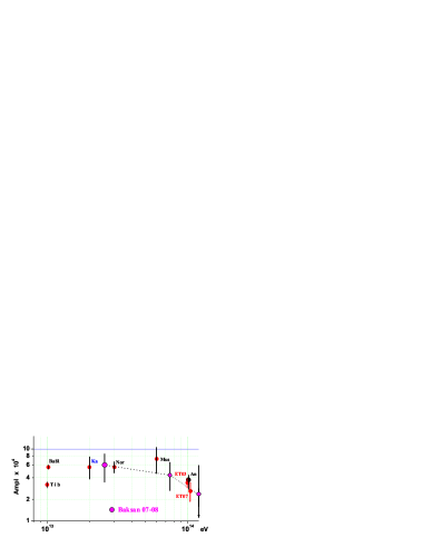
Figure 2: Amplitude of 1st harmonic of sidereal anisotropy for 10 -100 TeV energy range.

Ba81 - [7, 8], Tib - [13], Ka - [14],Nor - [4, 6], Mus - [5], ET03 - [11], ET07 - [2], An - [12]

Earlier EAS-TOP team also reported comparatively small amplitude [11] for E = 100 TeV. One year later Andyrchi result [12] for the same energy was presented being in excellent agreement with EAS-TOP one. It seems worthwhile to do some remarks on possible energy dependence of anisotropy. At 30th ICRC the EAS-TOP collaboration presented [2] results of reprocessed 8-year data set using E-W method - point ET07 at Fig.2. We can notice that this result together with previous ones for E = 100 TeV really indicate decreasing of amplitude for energy close to 100 TeV. And what is more interesting, with further increasing of energy the amplitude again increases up to 0.064 % at E = 400 TeV with drastic change in phase [2, 3] to 13.6 hour RA from 0.4 hour RA for 100 TeV. Apropos, such shift of phase was already pronounced in [11] for energy   300 TeV and higher but with less significance. Phase of max counting rate 0.4 hour RA for low energy corresponds to direction perpendicular to local Orion arm (in out of arm direction) and parallel to Galactic plane whereas 13.6 hour RA points to north Galactic Pole inside the local Galactic arm. Hence, it is possible to suppose that something changes in mechanism producing an anisotropy effect in primary cosmic ray flux at energy range 100 - 300 TeV. Obviously, to arrive at more definite conclusion we need acquire more data.

4 Conclusion

Posterior analysis demonstrates that ”East-West” method yields more reliable result on sidereal anisotropy in comparison with standard meteo correction method. Further accumulation of data is necessary to understand better the evolution of cosmic ray anisotropy in the energy range 10 - 100 TeV. Together with results from high energy range it will bring some new knowledge about origin and propagation of cosmic rays.

The work was supported in part by the RFBR grant N 06-02-16355, by the Government Contract N 02.445.11.7070 and by the RAS Basic Research Program ”Neutrino Physics”.

References

- [1] P.Ghia, ”Frontier Objects in Astrophysics and Particle Physics”, Italian Physical Society, 93(2007), p.475.
- [2] P.L Ghia (for EAS-TOP collaboration), report 1068, Proc.30th ICRC, Merida, Mexico, 2007.
- [3] M. Aglietta, V.V. Alekseenko, et al., submitted to APJL; astro-ph: arXiv: 0901.2740.
- [4] Sakakibara et al., Proc. 13th ICRC, Denver(1973), vol.2,pp.1058-1063.
- [5] Gombosi T. et al. ”Galactic cosmic ray anisotropy at eV”. Preprint KFKI-75-46, Central Research Institute for Physics, Budapest (1975).
- [6] Nagashima K. and Mori S. Proc. ICRSymp.,Tokyo (1976), pp.326-360.
- [7] Alexeenko V.V., Chudakov A.E., Gulieva E.N. and Sborshikov V.G. Proc.17th ICRC, Paris (1981),vol.2, pp.146-149.
- [8] Alexeenko V.V. and Navarra G. Let. Nuovo Cim., v.42, No.7(1985), pp.321-324.
- [9] Compton A.H. and Getting J.A. Phys.Rev., vol.47, No.11(1935),pp.817-821.
- [10] K.Nagashima et al. IL Nuovo Cim., v. 12 C, N. 6, Nov - Dic 1989.
- [11] EAS-TOP collaboration, Proc. 28th ICRC, 2003, Vol.1, pp.183-186.
- [12] V.A.Kozyarivsky et al.,Proc. 29 ICRC, Pune, 2005, v.2, pp.93-96; ArXiv:astro-ph/0406059.
- [13] Yi Zhang (for Tibet collaboration). ArXiv: astro-ph/0610671.
- [14] Y.Oyama. ArXiv: astro-ph/0605020.