Optimal leverage from non-ergodicity

Abstract

In modern portfolio theory, the balancing of expected returns on investments against uncertainties in those returns is aided by the use of utility functions. The Kelly criterion offers another approach, rooted in information theory, that always implies logarithmic utility. The two approaches seem incompatible, too loosely or too tightly constraining investors’ risk preferences, from their respective perspectives. The conflict can be understood on the basis that the multiplicative models used in both approaches are non-ergodic which leads to ensemble-average returns differing from time-average returns in single realizations. The classic treatments, from the very beginning of probability theory, use ensemble-averages, whereas the Kelly-result is obtained by considering time-averages. Maximizing the time-average growth rates for an investment defines an optimal leverage, whereas growth rates derived from ensemble-average returns depend linearly on leverage. The latter measure can thus incentivize investors to maximize leverage, which is detrimental to time-average growth and overall market stability. The Sharpe ratio is insensitive to leverage. Its relation to optimal leverage is discussed. A better understanding of the significance of time-irreversibility and non-ergodicity and the resulting bounds on leverage may help policy makers in reshaping financial risk controls.

This study focuses on the simple setup of self-financing investments, that is, investments whose gains and losses are reinvested without consumption or deposits of fresh funds, in assets undergoing geometric Brownian motion. The consequences of time irreversibility pertaining to studies of risk are discussed. Understanding these consequences appears particularly important in the light of the current financial and economic crisis. This will be elaborated at the end, in Sec. 4, after establishing the main concepts.

In Sec. 1 the portfolio selection problem, as introduced by Markowitz (1952), is reviewed. Its use of utility to express risk preferences is contrasted with a different ansatz, proposed by Kelly Jr. (1956), that makes use solely of the rôle of time in multiplicative processes. While in the terminology of modern portfolio theory, the latter ansatz can be interpreted as the assumption of logarithmic utility, in Sec. 1.1 the Kelly result is shown to be equivalent, in the present setup, to an application of Itô’s formula of stochastic calculus. In this sense it is not the reflection of a particular investor’s risk preferences but a generic null-hypothesis. Considerations of personal risk preferences can improve upon this hypothesis but they must not obscure the crucial rôle of time. In Sec. 2 it is shown by explicit calculation that the non-ergodicity of geometric Brownian motion can create a difference between ensemble-average and time-average growth rates. Itô’s formula is seen as a means to account for the effects of time. In Sec. 3 the growth-optimal leverage, which specifies a portfolio along the efficient frontier, is derived and related to a minimum investment time-horizon. Optimal leverage is compared to the Sharpe ratio. Finally, in Sec. 4 implications of the results from Sec. 3 for real investments are discussed, and the concept of statistical market efficiency is introduced.

1 Introduction

Modern portfolio theory deals with the allocation of funds among investment assets. We assume zero transaction costs and portfolios whose prices $p(t)$ follow geometric Brownian motion,

$$dp(t)=p(t)\left(\mu dt+\sigma dW_{t}\right),$$ (1)

where $\mu$ is a drift term, $\sigma$ is the volatility, and

$$W(T)\equiv\int_{t=0}^{t=T}dW_{t}$$ (2)

is a Wiener process.

Markowitz (1952) suggested to call a portfolio $i$ efficient if

a) there exists no other portfolio $j$ in the market with equal or smaller volatility, $\sigma_{j}\leq\sigma_{i}$, whose drift term $\mu_{j}$ exceeds that of portfolio $i$,

$$\text{for all~{}}j~{}\text{such that~{}}\sigma_{j}\leq\sigma_{i},\text{~{}we have~{}}\mu_{j}\leq\mu_{i}.$$ (3)

b) there exists no other portfolio $j$ in the market with equal or greater drift term, $\mu_{j}\geq\mu_{i}$, whose volatility $\sigma_{j}$ is smaller than that of portfolio $i$,

$$\text{for all~{}}j~{}\text{such that~{}}\mu_{j}\geq\mu_{i},\text{~{}we have~{}}\sigma_{j}\geq\sigma_{i}.$$ (4)

Markowitz (1952) argued that it is unwise to invest in any portfolio that is not efficient. In the presence of a riskless asset (with $\sigma_{i}$=0) all efficient portfolios lie along a straight line – the efficient frontier – that intersects, in the space of volatility and drift terms, the riskless asset, $R$, and the so-called market portfolio, $M$, (Tobin 1958), see Fig. 1.

Markowitz’ suggestion to focus on the mean $\mu$ and the variance $\sigma^{2}$ was later criticized because the first two moments alone do not sufficiently constrain the return distribution. Clearly preferable portfolios can appear inferior if assessed only by Markowitz’ 1952-criteria (Hanoch and Levy 1969). Below it will be stated specifically in what sense large $\mu$ and small $\sigma$ are desirable under the dynamics of (Eq. 1).

Since any point along the efficient frontier represents an efficient portfolio, Markowitz’ (1952) arguments need to be augmented with additional information in order to select the optimal portfolio. This additional information is generally considered a property of the investor, namely his risk preference, represented by a utility function, $u=u\left(p(t)\right)$, that specifies the usefulness or desirability of a particular investment outcome to a particular investor.

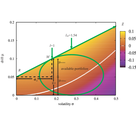
Figure 1: The efficient frontier (green straight line) intersects the the riskless asset $R$ (here $\mu_{\text{riskless}}=0.05$ per time unit) and is tangent to the space of available portfolios (green oval), touching at the point defined as the market portfolio, $M$ (here $\mu_{M}=0.1$ per time unit, resulting in an excess expected return of $M$ compared to $R$ of $\mu_{\text{excess}}=0.05$ per time unit; the volatility of the market portfolio $\sigma_{M}=0.18$ per square-root of time unit), corresponding to leverage $l=1$, left arrow. The color coding shows the expected, more specifically time-average, growth rate, $\bar{g}=\mu-\sigma^{2}/2$; the portfolio of optimal leverage (see Sec. 3, here $l_{\text{opt}}\approx 1.54$) along the efficient frontier is indicated by the right arrow. Both for fixed volatility $\sigma$ and fixed expected return, which we call the ensemble-average growth rate, $\mu$, there are no obtainable portfolios (those below the efficient frontier) whose time-average growth rates exceed that at the efficient frontier. Zero time-average growth rate is indicated white.

In a parallel development, Kelly Jr. (1956) considered portfolios that were also described by two parameters. In his case, the portfolios were double-or-nothing games on which one could bet an arbitrary fraction of one’s wealth (one parameter) and knew the outcome with some probability (second parameter). Both Markowitz (1952) and Kelly Jr. (1956) recognized that it is unwise to maximize what is often called the expected rate of return,

$$\left\langle g\right\rangle=\frac{1}{dt}\left\langle\frac{dp(t)}{p(t)}\right\rangle,$$ (5)

where $\left\langle\right\rangle$ denotes the ensemble mean over realizations of the Wiener process. Markowitz (1952) rejected such strategies because the portfolio with maximum expected rate of return is likely to be under-diversified. In Kelly’s case the probability of bankruptcy approaches one as games of maximum rate of return are repeated (Kelly Jr. 1956). In geometric Brownian motion bankruptcy is impossible, but the effects of time are essentially the same as in Kelly’s setup.

While Markowitz emphasized parameters such as risk preferences and personal circumstances (“The proper choice among portfolios depends on the willingness and ability of the investor to assume risk.” (Markowitz 1991)), Kelly used a fundamentally different ansatz by maximizing the so-called expected growth rate,

$$\bar{g}=\frac{1}{dt}\left\langle d\ln p\right\rangle,$$ (6)

rather than the expected rate of return, without an a priori need for additional information. The exact meaning of these two quantities will be worked out in Sec. 2, and a more precise nomenclature will be introduced shortly. The conditions under which the growth-rate ansatz alone yields meaningful results have been discussed in the literature (Merton and Samuelson 1974, Markowitz 1976, 1991). For self-financing portfolios (the focus of this study), where eventual outcomes are the product over intermediate returns, these conditions are met. This is a good approximation, e.g. for large pension funds where fluctuations in assets under management are dominated by market fluctuations (Schwarzkopf and Farmer 2008) and, arguably, for entire economies. Some stock market indeces, for example the DAX, also reflect the value of a hypothetical constant rebalanced self-financing portfolio with zero transaction costs. Equation (6) shows that the Kelly criterion, maximizing the expected growth rate, is mathematically similar to using logarithmic utility. In this special case, i.e. $u(p(t))=\ln\left(p(t)\right)$, the ensemble-average of the utility happens to be the time-average of the growth rate in a multiplicative process. The fact that the process is non-ergodic and the time-average has to be used explains why logarithmic utility so often yields intuitively sensible results, see Sec. 2.

The so-called Sharpe ratio, usually defined as $S=(\left\langle g\right\rangle-\mu_{\text{riskless}})/\sigma$, where $\mu_{\text{riskless}}$ is the rate of return on a riskless asset, is a means of analysis using Markowitz’ framework. It can be thought of as the slope of a straight line in Fig. 1 intersecting the riskless asset. We will return to the Sharpe ratio in Sec. 3.1, as it is best discussed using the main results about to be presented.

1.1 Two averages

In this section the reader is reminded that the two averages (Eq. 5) and (Eq. 6) are not necessarily identical. For riskless assets, the chain rule of ordinary calculus implies that (Eq. 5) and (Eq. 6) are identical, $\left\langle g\right\rangle_{\text{riskless}}=\bar{g}_{\text{riskless}}$, but this is not the case for non-zero volatility.

Combining (Eq. 1) and (Eq. 5), we now compute the expectation value of the fractional price increment per infinitessimal time step, the expected rate of return,

$$\left\langle g\right\rangle =\frac{1}{dt}\left\langle\frac{p(t)\mu dt+p(t)\sigma dW_{t}}{p(t)}\right\rangle$$ (7)

$$=\mu+\sigma\frac{1}{dt}\left\langle dW_{t}\right\rangle$$

$$=\mu.$$

From now on we will call this quantity the ensemble-average growth rate, for reasons that will be made clear in Sec. 2.

The object $d\ln p$ in (Eq. 6) has to be treated carefully using Itô’s formula. With the chain rule of ordinary calculus replaced by Itô’s version, (Eq. 5) and (Eq. 6) now correspond to different averages.

Itô’s formula for (Eq. 1), which we need to evaluate (Eq. 6), takes the form

$$df=\left(\frac{\partial f}{\partial t}+\mu p\frac{\partial f}{\partial p}+\frac{1}{2}\sigma^{2}p^{2}\frac{\partial^{2}f}{\partial p^{2}}\right)dt+p\sigma\frac{\partial f}{\partial p}dW_{t},$$ (8)

where $f=f(p(t),t)$ is some function of the Itô process $p(t)$ of (Eq. 1), and time $t$. The dependencies of $p(t)$ and $f(p(t),t)$ have been left out in (Eq. 8) to avoid clutter. The third term on the right of (Eq. 8) constitutes the difference from the increment for a function of a deterministic process. Due to the second derivative, Itô’s formula can only take effect if $f(p(t),t)$ is non-linear in $p$. To derive the increment $d\ln p$, we need to choose $f(p(t),t)\equiv\ln(p(t))$, that is, a non-linear function. We arrive at

$$d\ln p=\left(\mu-\frac{\sigma^{2}}{2}\right)dt+\sigma dW_{t}.$$ (9)

Notice that Itô’s formula changes the behavior in time, whereas the noise term is unchanged. In the literature, the corresponding average,

$$\bar{g} =\frac{1}{dt}\left\langle d\ln p\right\rangle$$ (10)

$$=\mu-\frac{\sigma^{2}}{2}+\frac{\sigma}{dt}\left\langle dW_{t}\right\rangle$$

$$=\mu-\frac{\sigma^{2}}{2},$$

is called the expected growth rate, or logarithmic geometric mean rate of return. Here we call it the time-average growth rate.

Distributions of logarithmic returns for many asset classes are highly non-Gaussian, see e.g. Mantegna and Stanley (1995). This does not affect the applicability of the concepts about to be discussed, however, as their justification is the irreversibility of time, see Sec. 2. In general, the time-average growth rate of a self-financed portfolio whose rates of return obey a given probability distribution is the logarithm of the geometric mean of that distribution, see e.g. Kelly Jr. (1956), Markowitz (1976). Extending the results of this study to return distributions that are not log-normal thus only requires the computation of the geometric mean.

Equation (10) shows that while the ensemble-average growth rate enters into the time-average growth rate, it does so in combination with the volatility, quantifying for the present setup the statement that large returns and small volatilities are desirable. This is illustrated in Fig. 1.

2 Ergodicity

How can we make sense of the difference between the quantities computed in (Eq. 7) and (Eq. 10) in the presence of non-zero volatility? The problem that additional information is needed to select the right portfolio, which was first treated by Bernoulli (1738), disappears when using (Eq. 10) – how did this problem arise in the first place, and what is the meaning of (Eq. 7)? It will be shown in this section that the non-ergodic nature of (Eq. 1) allows us to obtain $\left\langle g\right\rangle=\mu$ from an estimate for the growth rate averaged over an ensemble of infinitely many realizations of the stochastic process, whereas the time average of the same estimate produces $\bar{g}=\mu-\frac{\sigma^{2}}{2}$.

To generate the ensemble average, stochasticity is removed by letting the sample size, or number of realizations, or number of parallel universes diverge before the non-trivial effects of time, which arise from multiplicative noise, are fully taken into account. Equation (7) is thus the answer to the following question: “what is the rate of return on this investment, computed from an average over all possible universes?”, where a universe is defined as a particular sequence of events, i.e. one realization of the process (Eq. 1). This nomenclature is employed to emphasize that we only live in one realization of the universe but stay alive in that universe for some time. For most of us, therefore, this question is less relevant than the question: “what is the rate of return on this investment, averaged over time?”, to which the answer is (Eq. 10). This is illustrated in Fig. 2, where one realization of a self-financed portfolio is compared to an average over an increasing number of universes. This is achieved by producing independent sequences of wealth, corresponding to resetting an investor’s wealth and starting over again. The independent sequences are then averaged (arithmetically) at equal times. As this averaging procedure over universes destroys stochasticity, the stochastic exponential growth process (whose time-average growth rate is (Eq. 10)) approaches deterministic exponential growth (whose growth rate is the ensemble-average growth rate, (Eq. 7)). The procedure of starting over again is like going back in time, or periodically resetting one’s investment to its initial value. But going back in time is not possible, and the self-financing portfolios considered here do not allow any resetting. For processes with Wiener noise, (Eq. 2), Itô’s formula can encode the multiplicative effect of time in the ensemble average. These intuitive arguments will now be made precise.

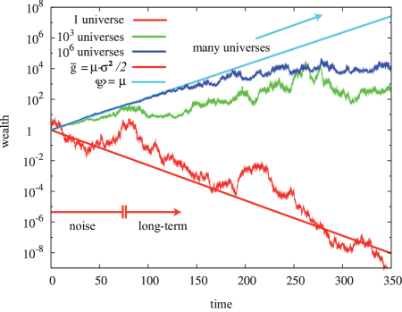
Figure 2: Wealth starts at unity at time $T=0$ and then behaves according to (Eq. 1) with $\mu=0.05$ per time unit and volatility $\sigma=0.45$ per square root of one time unit, implying the time-average exponential growth rate $\bar{g}\approx-0.051$ per time unit. For short times the performance is noise-dominated; after $T\approx 75$ time units (red arrow, (Eq. 19)) the time-average growth rate takes over (see also Fig. 3). To uncover the ensemble-average growth rate (Eq. 5) from the dynamics, an average over many independent universes must be taken.

Ergodicity requires a unique stationary probability distribution of the process $p(T)$ in the long-time limit $T\to\infty$. Geometric Brownian motion is therefore trivially non-ergodic because it is not a stationary process. This implies that there is no guarantee for the ensemble average of an observable to be identical to its time average. The observable we are interested in is the growth rate. It will be shown that (Eq. 5) corresponds to the ensemble average of a particular estimator for the growth rate, and that (Eq. 6) corresponds to the time average.

In practice, an exponential growth rate is estimated from observations over a finite time $T$. To add the possibility of averaging over $N$ parallel universes (or completely independent systems), we consider the estimator

$$g_{\text{est}}(T,N)=\frac{1}{T}\ln\left\langle\frac{p(T)}{p(0)}\right\rangle_{N}.$$ (11)

Here, the angled brackets denote the average over $N$ realizations, $\left\langle\right\rangle_{N}=\frac{1}{N}\sum_{i=1}^{N}$. The different $p_{i}(T)$ are obtained by solving the stochastic differential equation (Eq. 1) by integrating (Eq. 9) over time and then exponentiating,

$$p_{i}(T)=p(0)\exp\left(\left(\mu-\frac{\sigma^{2}}{2}\right)T+\sigma W_{i}(T)\right).$$ (12)

The sample average in (Eq. 11) must not enclose the logarithm. The quantity that reveals the non-ergodic properties of (Eq. 1) and clarifies the meaning of (Eq. 5) is obtained by averaging the values $p_{i}(T)$ from individual realizations, $i$, first, before the logarithm translates them into a growth rate. This procedure corresponds precisely to Fig. 2, where outcomes $p_{i}(T)$ are averaged first at equal times, and then a growth rate is derived by taking the logarithm. This is different from Bernoulli’s treatment, where the logarithm is a utility function and would be inside the sample average, obscuring the conceptual failure of the ensemble-average. It was Kelly Jr. (1956) who first pointed out that the time average should be considered instead.

The ensemble average of the estimator (Eq. 11) can be identified with the limit

$$\left\langle g\right\rangle=\lim_{N\to\infty}g_{\text{est}}(T,N),$$ (13)

whereas the time average results from the limit

$$\bar{g}=\lim_{T\to\infty}g_{\text{est}}(T,N=1).$$ (14)

Writing the averages as these two limits helps elucidate the relation between (Eq. 5) and (Eq. 6), and it shows the symmetry or absence thereof between effects of additional time and effects of additional parellel universes included in the estimate. We will now calculate both to show explicitly that the limits are not interchangeable. We start with the ensemble-average. The Wiener process $W(T)$ in (Eq. 2) is Gaussian-distributed with mean 0 and standard deviation $\sqrt{T}$. Using the fundamental transformation law of probabilities, (Eq. 12) thus implies that $\left(\frac{p(T)}{p(0)}\right)$ is log-normally distributed, according to

$$P\left(\frac{p(T)}{p(0)}\right)=\frac{1}{\left(\frac{p(T)}{p(0)}\right)\sqrt{2\pi T\sigma^{2}}}\exp\left(-\frac{\left(\ln\left(\frac{p(T)}{p(0)}\right)-(\mu-\frac{\sigma^{2}}{2})T\right)^{2}}{2T\sigma^{2}}\right).$$ (15)

The first moment of $\left(\frac{p(T)}{p(0)}\right)$ is

$$\lim_{N\to\infty}\left\langle\frac{p(T)}{p(0)}\right\rangle_{N}=\exp(\mu T),$$ (16)

the well known expectation value of log-normally distributed variables. Using this in (Eq. 13) in conjunction with (Eq. 11) yields

$$\left\langle g\right\rangle =\mu$$ (17)

$$=\frac{1}{dt}\left\langle\frac{dp(t)}{p(t)}\right\rangle,$$

where the last line follows from (Eq. 7), explaining our nomenclature of referring to (Eq. 5) as an ensemble-average growth rate.

Next, we consider (Eq. 14), where the long-time limit is responsible for eliminating stochasticity. Using $N=1$ since we are interested only in one realization that could be our reality, and substituting (Eq. 11) and (Eq. 12) in (Eq. 14) we find

$$\bar{g} =\lim_{T\to\infty}\frac{1}{T}\left(\left(\mu-\frac{\sigma^{2}}{2}\right)T+\sigma W(T)\right)$$ (18)

$$=\mu-\frac{\sigma^{2}}{2}+\lim_{T\to\infty}\left(\sigma T^{-1/2}W(1)\right)$$

$$=\mu-\frac{\sigma^{2}}{2}$$

$$=\frac{1}{dt}\left\langle d\ln p\right\rangle.$$

The step from line one to two in (Eq. 18) follows from the scaling properties of Brownian motion. Although clearly $W(T)$ cannot be equated to $T^{1/2}W(1)$ for any specific realization, the step is valid because of the limit $T\to\infty$. The final line follows from (Eq. 10), and we identify the time-average growth rate with (Eq. 6). The decay of the stochastic term as $T^{-1/2}$ is illustrated in Fig. 3.

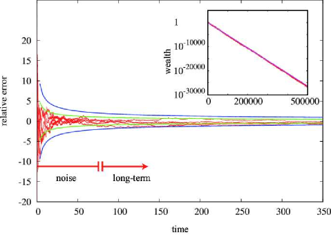
Figure 3: Relative errors $\frac{g_{\text{est}}(T,N=1)-\bar{g}}{\bar{g}}$ in estimates of the time-average growth rate, using the estimator $g_{\text{est}}(T,N=1)=\frac{1}{T}\ln\left(\frac{p(T)}{p(0)}\right)$ in single realizations of the process described in the caption of Fig. 2. Green lines show one relative standard deviation from expected estimates, $\frac{\sigma T^{-1/2}}{\bar{g}}$, blue lines show two standard deviations.
Inset: Long-time averages approach deterministic behavior with the time-average growth rate.

Equation (12) shows that the median of $\left(\frac{p(T)}{p(0)}\right)$ is $\exp\left(\left(\mu-\frac{\sigma^{2}}{2}\right)T\right)$. But this is not the expectation value, as the multiplicative nature of the process makes for very large, though unlikely, positive fluctuations, and in the ensemble but not in time these off-set the term $-\frac{\sigma^{2}}{2}T$. Interpreting this in an investment context exposes the dangers of misinterpreting (Eq. 5) and (Eq. 6): using the ensemble-average growth rate where the time-average growth rate would be appropriate overestimates the effect of positive fluctuations. Extreme situations can be envisaged, where the investor is bound to lose everything, although from the perspective of the ensemble average, a few lucky copies of him in parallel universes make up for his loss, making an investment proposition seem attractive (Peters 2009). But because resources cannot be exchanged with other members of the ensemble (in parallel universes), this offset is of no use to the investor as he progresses through time.

Using the estimator (Eq. 11), we have shown that (Eq. 5) is an ensemble-average growth rate where stochasticity is removed by the limit $N\to\infty$ and the effects of time are suppressed. Equation (6) is the time-average growth rate, where stochasticity is removed by the limit $T\to\infty$. The difference between the two explicitly calculated growth rates, i.e. the fact that the limits $\lim_{N\to\infty}$ and $\lim_{T\to\infty}$ do not commute, is a manifestation of the non-ergodicity of the system. Both rates can be obtained as ensemble-averages as in (Eq. 7) and (Eq. 10); in differential form, the ensemble-average growth rate is straight-forward, whereas the time-average growth rate requires the application of Itô’s formula. Intuitively, Itô’s formula corresponds to the inclusion of effects of ignorance regarding the future (see Lau and Lubensky (2007), Øksendal (2005), Ch. 3), and it encodes the effect of time correctly for noise terms of the type of (Eq. 2).

At zero volatility the “time-average” (certain) growth rate equals the ensemble-average growth rate, and any investor will choose the highest-yielding portfolio available, maximizing both the time-average growth rate and the ensemble-average growth rate over all possible universes (there is only one possible universe now). Generalizing to the stochastic case, it is still sensible to maximize time-average growth rates, but this is not equivalent to maximizing ensemble-average growth rates. A good guide, whether investing with or without volatility, is concern for the future, rather than concern for copies of oneself in parallel universes.

3 Minimum investment horizon and optimal leverage

Logarithmic utility, the Kelly criterion and time-average growth rates are often associated with “long-term investment”. The long term here means a time scale that is long enough for the deterministic part of the exponent in (Eq. 12) to dominate over the noise. Applying this terminology to the present case, one is investing either for the long term, or in a regime where randomness dominates – the latter case may be described as “gambling”. If in (Eq. 12), the $W(T)$ is replaced by $\sqrt{\left\langle W(T)^{2}\right\rangle}=\sqrt{T}$, we estimate that gambling stops, and the long term begins when

$$t>t_{c}=\frac{\sigma^{2}}{\left(\mu-\frac{\sigma^{2}}{2}\right)^{2}}.$$ (19)

In Fig. 2 the corresponding time scale is $t_{c}\approx 75$ time steps, indicated by the break in the red arrow. At this point, the typical relative error in estimates $g_{\text{est}}(T,N=1)$ of $\bar{g}$ based on past performance is unity, indicated by a break in the arrow in Fig. 3. In a single universe, such as our reality, the system is never dominated by the ensemble-average growth rate – neither in the short run nor in the long run. Instead, there is an initial noise-regime where no significant trends can be discerned, whereafter the time-average growth rate dominates the performance.

Equation (19) indicates how long we must expect to wait for the trend of the market to become distinguishable from fluctuations, wherefore $t_{c}$ may be viewed as a minimum investment horizon. The parameters of Fig. 1, with a time unit of one year, imply $t_{c}\approx 4.6$ years. Historical comparisons between portfolios with similar stochastic properties are meaningful only on much longer time scales.

The use of the null model of maximizing the time-average growth rate eliminates the a priori need to specify risk-preferences. Tailoring real-life investments to real investors’ needs does require difficult to formalize knowledge of their circumstances, but a number of issues can be illuminated without such knowledge in the simple context of the null-hypothesis. For instance, a well-defined optimal leverage can be computed as will be shown now. The result follows directly from Kelly’s (1956) arguments, and several authors have come to the same conclusions using different methods (Kestner 2003, Thorp 2006). In addition, the characteristic time scale of (Eq. 19) is calculated for the leveraged case, which defines a critical leverage where the expected growth rate vanishes.

Any efficient portfolio along the straight efficient frontier can be specified by its fractional holdings of the market portfolio (Sharpe 1964), which we define as the leverage, $l$. For instance, an investor who keeps all his money in the riskless asset holds a portfolio of leverage $l=0$; half the money in the riskless asset and half in the market portfolio is leverage $l=0.5$, and borrowing as much money as one owns and investing everything in the market portfolio corresponds to $l=2$ etc.

The ensemble-average growth rate in the leveraged case can be written as the sum $\mu_{\text{riskless}}+l\mu_{\text{excess}}$, where $\mu_{\text{excess}}$ is the excess ensemble-average growth rate of the market portfolio over the riskless growth rate, see Fig. 1. At zero leverage, only the riskless growth rate enters; the excess ensemble-average growth rate is added in proportion to the leverage. Noting that both the ensemble-average growth rate and the volatility depend linearly on the leverage, we obtain the leveraged stochastic process

$$dp_{l}(t)=p_{l}(t)\left(\mu_{\text{riskless}}+l\mu_{\text{excess}})dt+l\sigma_{M}dW_{t}\right),$$ (20)

where $\sigma_{M}$ is the volatility of the market portfolio. Just like with (Eq. 1), we can use Itô’s formula, (Eq. 8), to derive the equation of motion for the logarithm of the price, $p_{l}(t)$, of the leveraged portfolio,

$$d\ln p_{l}=\left(\mu_{\text{riskless}}+l\mu_{\text{excess}}-\frac{l^{2}\sigma_{M}^{2}}{2}\right)dt+l\sigma_{M}dW_{t}.$$ (21)

The time-average leveraged exponential growth rate is thus

$$\bar{g_{l}} =\frac{1}{dt}\left\langle d\ln p_{l}\right\rangle$$ (22)

$$=\left(\mu_{\text{riskless}}+l\mu_{\text{excess}}-\frac{l^{2}\sigma_{M}^{2}}{2}\right).$$

The positive contribution to $\bar{g_{l}}$ is linear in the leverage, but the negative contribution is quadratic in the leverage. The quadratic term is an effect of time and makes the time-average growth rate non-monotonic in the leverage.

Markowitz (1952) rejected strategies of maximum ensemble-average growth because the corresponding portfolios are likely to be under-diversified and hence to have an unacceptably high volatility. Equation (22) shows that in the limit of large leverage, seeking high ensemble-average growth rates, the time-average growth rate along the efficient frontier diverges negatively, as $\lim_{l\to\infty}\bar{g_{l}}/l^{2}=-\sigma_{M}^{2}/2<0$.

To find the optimal leverage, we differentiate (Eq. 22) with respect to $l$ and set the result to zero, obtaining

$$l_{\text{opt}}=\mu_{\text{excess}}/\sigma_{M}^{2}.$$ (23)

The second derivative of (Eq. 22) with respect to $l$ is $-\sigma_{M}^{2}$, which is always negative, implying that $\bar{g_{l}}$ corresponding to $l_{\text{opt}}$ is maximized. This calculation shows that there exists a privileged portfolio along the efficient frontier. If the market portfolio has a lower volatility than the portfolio of maximum time-average growth rate, as in Fig. 1, then the wise investor will leverage his position by borrowing ($l_{\text{opt}}>1$). If, on the other hand, the market portfolio has a higher volatility, as in Fig. 2, then he will keep some fraction of his money safe ($l_{\text{opt}}<1$).

We note that in geometric Brownian motion $\bar{g}$ can never be increased by decreasing $\mu$ at constant volatility, nor can it be increased by increasing volatility at constant $\mu$, because from (Eq. 10), $\frac{\partial\bar{g}}{\partial\mu}>0$ and $\frac{\partial\bar{g}}{\partial\sigma}<0$. Therefore, the globally (i.e. selected from all possible portfolios) growth-optimal portfolio will be located on the efficient frontier. This temporal optimization thus does not contradict modern portfolio theory. For the dynamics of (Eq. 1) it confirms (Eq. 3) and (Eq. 4) as the definition of efficient, i.e. potentially optimal, portfolios.

Including the leverage in (Eq. 19) results in the leveraged characteristic time scale separating gambling from investing

$$t_{c}^{l}=\frac{l^{2}\sigma_{M}^{2}}{\left(\mu_{\text{riskless}}+l\mu_{\text{excess}}-\frac{l^{2}\sigma_{M}^{2}}{2}\right)^{2}}.$$ (24)

This time scale diverges at the critical leverages,

$$l_{c}^{\pm}=l_{\text{opt}}\pm\sqrt{l_{\text{opt}}^{2}+2\left(\frac{\mu_{\text{riskless}}}{\sigma_{M}^{2}}\right)}$$ (25)

We are interested especially in the positive root, $l_{c}^{+}$, where the time-average leveraged growth rate (the denominator of (Eq. 24)) is zero due to over-leveraging. The minimum investment horizon (Eq. 24) becomes infinite, meaning that such an investment will forever be a gamble. The parameters of Fig. 1, for example, imply $l_{c}^{+}\approx 3.88$, where the extrapolations of the white and green lines in the figure cross.

For leverages, $l>l_{c}^{+}$, the time-average growth rate is negative, and the time scale (Eq. 24) is finite and marks the transition between noise and discernible loss of invested capital. This is the case in Fig. 2, where $l_{\text{opt}}\approx 0.25$, the critical leverage $l_{c}\approx 0.49$, the system runs at $l=1$, and $t_{c}^{l=1}\approx 75$ time units.

3.1 Sharpe Ratio

The results from Sec. 3 also yield insights into the Sharpe ratio, mentioned in Sec. 1. Writing in 1966, Sharpe suggested to assess the quality of a portfolio specified by some $\mu$ and $\sigma$ using the slope of the straight line in the $\mu$ vs. $\sigma$ plane in Fig. 1 that corresponds to combinations of the portfolio and the riskless asset (i.e. to all possible values of $l$),

$$S=\frac{\mu-\mu_{\text{riskless}}}{\sigma}.$$ (26)

The concept of ergodicity is relatively young, with major results in ergodic theory emerging in the second half of the 20${}^{\text{th}}$ century (Lebowitz and Penrose 1973). For early roots of the discussion, see Uffink (2004). The concepts did not immediately diffuse into the economics literature: in the 1966 paper Sharpe makes no distinction between time- and ensemble-averages. It is assumed here that he refers to ensemble averages throughout the paper. Some authors assume that he refers to time-averages (Bouchaud and Potters 2000), but the resulting quantity, $\frac{\mu-\frac{\sigma^{2}}{2}-\mu_{\text{riskless}}}{\sigma}$, has a less straight-forward meaning. Despite the exclusive use of ensemble averages in (Eq. 26), $S$ is also meaningful in the context of time averages in geometric Brownian motion: given two portfolios $M_{1}$ and $M_{2}$, where $S(M_{1})>S(M_{2})$, the optimally leveraged portfolio $M_{1}^{l_{\text{opt 1}}}$ always has a greater time-average growth rate than the optimally leveraged portfolio $M_{2}^{l_{\text{opt 2}}}$.

Sharpe was fully aware of the limitations of his measure: $S(M_{1})>S(M_{2})$ does not mean that an investment in $M_{1}$ will outperform an investment in $M_{2}$, as it is possible that $M_{1}$ is far from optimally leveraged. He concluded that “The investor’s task is to select from among the efficient portfolios the one that he considers most desirable [i.e. to choose a leverage $l$], based on his particular feelings regarding risk and expected return (Sharpe 1966).” Without considerations of ergodicity, investors are indeed left to making decisions based on their feelings.

The optimal leverage $l_{\text{opt}}=\frac{\mu_{\text{excess}}}{\sigma_{M}^{2}}$, differs from the Sharpe ratio (Eq. 26) for the market portfolio only by a square in the volatility. Indeed, it may also be considered a fundamental measure of the quality of a portfolio: if the optimal leverage for a given investment opportunity is high, then this is a good opportunity that calls for a large commitment.

Optimal leverage, unlike the Sharpe ratio, is a dimensionless quantity. This is a significant difference, as it implies that the numerical value of optimal leverage, which is a pure number, can distinguish between fundamentally different dynamical regimes, see e.g. Barenblatt (2003). For example, a value $l_{\text{opt}}<1$, irrespective of its constituting $\sigma_{M}$ and $\mu_{\text{excess}}$, or the unit of time used to measure these quantities, implies that an investor will be better off keeping some of his money safe. The Sharpe ratio, (Eq. 26), on the other hand, has dimension $[S]=\mathrm{T}^{-1/2}$, wherefore it depends on the chosen unit of time, implying that its numerical value is arbitrary. For example, a portfolio with Sharpe ratio 5, where $\mu$ is measured as a percentage per year and $\sigma$ as a percentage per square-root of one year would have Sharpe ratio $\frac{5}{\sqrt{365}}\approx 0.26$ if the chosen time unit were one day.

In the context of the current crisis the limitation of the Sharpe ratio is perhaps best expressed by its insensitivity to leverage,

$$S_{l}=\frac{l(\mu-\mu_{\text{riskless}})}{l\sigma}=S.$$ (27)

Using the Sharpe ratio alone to assess the quality of an investment would be dangerous, as this measure cannot detect the negative effects of leverage. Given the systemic incentives for using large leverage, this insensitivity can become a danger to market stability.

4 Discussion

Practically relevant lessons from the above considerations may be learned from the extremes. A 100% mortgage, for instance, corresponds to infinite leverage, implying $\bar{g}\to-\infty$, on the borrower’s investment (assuming that the purchase is not part of a larger investment portfolio). Although total loss on a home purchase only means dipping into negative equity, certain financial products that have become popular in recent years must be regarded as irresponsible. Conversely, (Eq. 22) shows that for $l\ll 1$ the time-average growth rate is well approximated by the ensemble average. From the very beginning, treatments of gambling focused on ensemble-average outcomes, e.g. Cardano’s 16${}^{\text{th}}$ century “Liber de Ludo Aleae”, translated by Gould in Ore (1953). This is appropriate as long as wagers are much less than total wealth, meaning leverage close to zero, where $\bar{g}$ becomes indistinguishable from $\left\langle g\right\rangle$.

The current financial crisis started in the summer of 2007, with the US housing market collapsing and the visible consequence of Northern Rock in the UK suddenly unable to raise credit, i.e. leverage, on the open market. Subsequently, credit markets began to freeze. After the nationalization of Fannie Mae and Freddie Mac and the bankruptcy of Lehman Brothers in September 2008 entire markets for leverage-oriented financial products disappeared (securitization and credit default swaps, for instance, were strongly affected). Leverage clearly played a big rôle. The scale of this crisis suggests to revisit some of the basic tenets of the economic formalism, including the concept of equilibrium, the rôle of time, and indeed the frequent implicit assumption of ergodicity.

It is emphasized here that ergodicity can be inadvertently assumed by writing an expectation value $\left\langle\right\rangle$, which implies the limit $N\to\infty$ of infinitely many realizations of a process. The straight-forward expected outcome, $\left\langle p(T)\right\rangle=\int pP(p)dp$, of some investment is indeed an average over many universes. Even if subsequently an exponential growth rate is derived from this as $\frac{1}{T}\ln\left(\frac{\left\langle p(T)\right\rangle}{p(0)}\right)$, the multiplicative effects of time are ignored, and the result will not be the time-average growth rate. We have seen that this problem persists, even if Itô’s formula is used to find the distribution of $p(T)$.

Real portfolios of constant leverage (apart from $l=0$ and possibly $l=1$) need to be constantly rebalanced as the value of the market portfolio fluctuates and changes the fraction of wealth invested in it. Holding any such portfolio is costly, both in terms of monitoring time and in terms of transaction costs. For applications, the above considerations would thus need to be adapted, even if real prices were perfectly described by (Eq. 1). The value of real optimal leverage depends on the investor’s ability to balance portfolios, which is affected by the available technology and, due to market impact, by the volume of the investment. The assumptions made in this study are likely to lead to an over-estimate of optimal leverage: Equation (23) was derived in continuous time, corresponding to truly constantly rebalanced portfolios, zero transaction costs were assumed, log-normal return-distributions, certain knowledge of $\mu$ and $\sigma$, and no risk premiums charged on money borrowed for leveraging.

Modelling the S&P500 or the DJIA with (Eq. 1), one would choose parameters close to those of Fig. 1 with time units of one year. This implies an optimal leverage, as calculated above, of 1.54, but it is unlikely that the simple strategy of borrowing money and investing it in the S&P500 would outperform the market. It is equally unlikely that investing only part of one’s money in the S&P500 would outperform the market, as would be the case if $l_{\text{opt}}<1$. A reasonable guess is that real optimal leverage is close to $l_{\text{opt}}=1$, a possible attractor for a self-organized market system. How could such statistical market efficiency work? If $l_{\text{opt}}>1$, money will be borrowed to be invested. This situation can arise as a consequence of low interest rates and low-cost credit. Leverage tends to increase volatility due to potential margin calls and similar constraints on investors (Geanakoplos 1997). Thus, as investors increase their leverage, they reduce optimal leverage, creating a negative feedback loop whose strength depends on the magnitude of the impact of leverage on volatility (“$\frac{d\sigma}{dl}$”), this brings optimal leverage down, $l_{\text{opt}}\to 1^{+}$. Conversely, if optimal leverage is less than unity, investors will sell risky assets, thereby reducing prices and increasing expected returns, such that optimal leverage increases, possibly up to $l_{\text{opt}}\to 1^{-}$.

The time scales associated with such a feedback loop can be long, especially in situations where leverage initially reduces volatility. The current financial crisis has been related to a continued extension of credit (Soros 2008a, b), i.e. increasingly leveraged investments. Effects of leverage that are initially volatility-reducing can be discussed in terms of mortgages: easy availability of mortgages increases house prices, which leads to few defaults, even if loans are given to borrowers who cannot service them from wages. In turn, because volatility decreases, optimal leverage increases, and houses appear a good investment. Consequently, more money is lent to home buyers, leading to a destabilizing run-away dynamics. Soros (2008a) has called such interaction between the asset price and the investment in the asset (the loan) “reflexivity”. After this initial reflexive phase of bubble creation, leverage will be perceived in some areas to have risen far beyond optimality, creating an unstable market situation. The ensuing crisis may be viewed as a response where volatility suddenly increases, reducing optimal leverage, which in turn leads to deleveraging and falling prices.

The use of leverage is not fundamentally constrained by the prevailing framework of portfolio selection, which relies on a necessarily and explicitly subjective notion of optimality, dependent on utility, or risk preferences. This has become problematic because asymmetric reward structures have encouraged excessive leveraging. Securitization, for example, creates such structures by separating the sellers of leverage products (such as mortgages), who are rewarded for every sale, from those who eventually bear the risk. Similarly, an investment manager who benefits from gains in the account he manages but is not personally liable for losses has an incentive to exceed growth-optimal leverage (see footnote on p. 5). In the ideal setup discussed above, the growth-optimal ansatz suggests a simple reward scheme through alignment of interests: requiring investment managers to invest all their wealth in the accounts managed by them. It is thereby achieved that the growth-optimal investment strategy for the account is also growth optimal for the investment manager. It is commonly said that excessive leverage arises when investors are short-term oriented, but there is no benefit from leveraging beyond optimality even in the short term – this regime is dominated by noise, not by ensemble-average growth rates. It is harmless to reward investment managers daily, hourly or indeed continuously for their performance – as long as they share the risks as much as the rewards.

Equation (22) carries an important message regarding reward structures in the financial industry. Excessive leverage leads to large fluctuations in asset prices but also more generally in economic output (the current recession being a case in point). The introduction of such fluctuations must reduce time-average economic growth. Remuneration practices have been criticized on a moral basis, using concepts like greed, excess and inequality. Objectively one can argue that remuneration structures can go against the common good by reducing economic growth by generating unnecessary fluctuations.

In conclusion, utility functions were introduced in the early 18${}^{\text{th}}$ century to solve a problem that arose from using ensemble averages where time averages seem more appropriate. Much of the subsequently developed economic formalism is limited by a similar use of ensemble averages and often overlooks the general problem that time- and ensemble averages need not be identical. This issue was treated in detail only in the 20${}^{\text{th}}$ century in the field of ergodic theory. Making use of this work, a privileged portfolio uniquely specified by an optimal leverage and a maximized time-average growth rate is seen to exist along the efficient frontier, the advantages of which have also been discussed elsewhere (Breiman 1961, Merton and Samuelson 1974, Cover and Thomas 1991). The concept of many universes is a useful tool to understand the limited significance of ensemble averages. While modern portfolio theory does not preclude the use of, in its nomenclature, logarithmic utility, it seems to underemphasize its fundamental significance. It was pointed out here that the default choice to optimize the time-average growth rate is physically motivated by the passage of time and the non-ergodic nature of the multiplicative process.

References

- Barenblatt (2003) Barenblatt, G.I., Scaling 2003, Cambridge University Press.
- Bernoulli (1738) Bernoulli, D., Specimen Theoriae Novae de Mensura Sortis. Translation “Exposition of a New Theory on the Measurement of Risk” by L. Sommer (1956). Econometrica, 1738, 22, 23–36.
- Bouchaud and Potters (2000) Bouchaud, J.P. and Potters, M., Theory of financial risks 2000, Cambridge University Press.
- Breiman (1961) Breiman, L., Optimal gambling systems for favorable games. In Proceedings of the Fourth Berkeley Symposium, pp. 65–78, 1961.
- Cover and Thomas (1991) Cover, T.M. and Thomas, J.A., Elements of Information Theory 1991, Wiley & Sons.
- Geanakoplos (1997) Geanakoplos, J., Promises promises. In The Economy as an Evolving Complex Systems II, SFI Studies in the Sciences of Complexity, edited by B. Arthur, Durlauf and D. Lane, pp. 285–320, 1997, Adddison-Wesley.
- Hanoch and Levy (1969) Hanoch, G. and Levy, H., The efficiency analysis of choices involving risk. Rev. Econ. Stud., 1969, 36, 335–346.
- Hull (2006) Hull, J.C., Options, Futures, and Other Derivatives, 6 2006, Prentice Hall.
- Kelly Jr. (1956) Kelly Jr., J.L., A New Interpretation of Information Rate. Bell Sys. Tech. J., 1956, 35.
- Kestner (2003) Kestner, L., Quantitative Trading Strategies 2003, McGraw-Hill.
- Lau and Lubensky (2007) Lau, A.W.C. and Lubensky, T.C., State-dependent diffusion: Thermodynamic consistency and its path integral formulation. Phys. Rev. E, 2007, 76, 011123.
- Lebowitz and Penrose (1973) Lebowitz, J.L. and Penrose, O., Modern ergodic theory. Phys. Today, 1973, pp. 23–29.
- Mantegna and Stanley (1995) Mantegna, R.N. and Stanley, H.E., Scaling behavior in the dynamics of an economic index. Nature, 1995, 376, 46–49.
- Markowitz (1952) Markowitz, H., Portfolio Selection. J. Fin., 1952, 1, 77–91.
- Markowitz (1976) Markowitz, H.M., Investment for the Long Run: New Evidence for an Old Rule. J. Fin., 1976, 31, 1273–1286.
- Markowitz (1991) Markowitz, H.M., Portfolio Selection, Second 1991, Blackwell Publishers Inc.
- Merton and Samuelson (1974) Merton, R.C. and Samuelson, P.A., Fallacy of the log-normal approximation to optimal portfolio decision-making over many periods. J. Fin. Econ., 1974, 1, 67–94.
- Øksendal (2005) Øksendal, B., Stochastic Differential Equations, 6th ed. 2003, Corrected 3rd printing 2005, Springer.
- Ore (1953) Ore, O., Cardano the gambling scholar 1953, Princeton University Press.
- Peters (2009) Peters, O., On time and risk. Bulletin of the Santa Fe Institute, 2009, 24, 36–41.
- Schwarzkopf and Farmer (2008) Schwarzkopf, Y. and Farmer, D., Time evolution of the mutual fund size distribution. available at SSRN: http://ssrn.com/abstract=1173046 2008.
- Sharpe (1964) Sharpe, W.F., Capital Asset Prices: A Theory of Market Equilibrium under Conditions of Risk. J. Fin., 1964, 19, 425–442.
- Sharpe (1966) Sharpe, W.F., Mutual fund performance. J. Business, 1966, 39, 119–138.
- Soros (2008a) Soros, G., The crisis and what to do about it. New York Rev. Books, 2008a, 55.
- Soros (2008b) Soros, G., The new paradigm for financial markets – the credit crisis of 2008 and what it means 2008b, PublicAffairs.
- Thorp (2006) Thorp, E.O., Vol. 1, 9 – The Kelly criterion in blackjack, sports betting, and the stock market. In Handbook of Asset and Liability Management: Theory and Methodology, 2006, Elsevier.
- Timmermann (1993) Timmermann, A.G., How Learning in Financial Markets Generates Excess Volatility and Predictability in Stock Prices. Quart. J. Econ., 1993, 108.
- Tobin (1958) Tobin, J., Liquidity Preference as Behavior Towards Risk. Rev. Econ. Stud., 1958, 25, 65–86.
- Uffink (2004) Uffink, J., Boltzmann’s Work in Statistical Physics. 2004, Technical report, Stanford Encyclopedia of Philosophy.
- van Kampen (1992) van Kampen, N.G., Stochastic Processes in Physics and Chemistry 1992, Elsevier (Amsterdam).