First-principle solubilities of alkali and alkaline earth metals in Mg-B alloys

Abstract

By devising a novel framework, we present a comprehensive theoretical study of solubilities of alkali (Li, Na, K, Rb, Cs) and alkaline earth (Be, Ca, Sr, Ba) metals in the he boron-rich Mg-B system. The study is based on first-principle calculations of solutes formation energies in MgB₂, MgB₄, MgB₇ alloys and subsequent statistical-thermodynamical evaluation of solubilities. The advantage of the approach consists in considering all the known phase boundaries in the ternary phase diagram. Substitutional Na, Ca, and Li demonstrate the largest solubilities, and Na has the highest (0.5-1 % in MgB₇ at $T=650-1000$ K). All the considered interstitials have negligible solubilities. The solubility of Be in MgB₇ can not be determined because the corresponding low-solubility formation energy is negative indicating the existence of an unknown ternary ground state. We have performed a high-throughput search of ground states in binary Mg-B, Mg-$A$, and B-$A$ systems, and we construct the ternary phase diagrams of Mg-B-$A$ alloys based on the stable binary phases. Despite its high temperature observations, we find that Sr₉Mg₃₈ is not a low-temperature equilibrium structure. We also determine two new possible ground states CaB₄ and RbB₄, not yet observed experimentally.

I Introduction

The interest in magnesium diboride emerged after the discovery of superconductivity in MgB₂ at about $T_{c}$=39 K.MgB2-2001 Attempts to increase $T_{c}$ by small additions of alkali (LiOwens01Li ; Zhao01Li ; Zhang02CaLi ; Cimb02Li ; Karp08Li , NaToul02NaCa ; Agost07Na , RbPalnich07RbCsBa ; Singh08RbCs , CsPalnich07RbCsBa ; Singh08RbCs ) and alkaline earth (BeFeln01Be , CaToul02NaCa ; Zhang02CaLi ; Cheng03Ca ; Tamp03CaSr , BaPalnich07RbCsBa ) metals to MgB₂, proved to be unsuccessful. The difficulty was attributed not only to the inability of such solutes to decrease $T_{c}$ but also to their low solubility and precipitation in secondary phases. Although a claimed superconductivity at 50K was reported for the Mg-B-$A$ ($A$=Cs, Rb, Ba) system Palnich07RbCsBa , attempts to reproduce the results have been so far unsuccessful (for $A$=Cs, Rb) Singh08RbCs . The problem can be attributed to solutes’ segregation in grain boundaries and to thus to low solubility in the bulk phase (much lower than reported in Ref. Palnich07RbCsBa, ).

For consistent interpretation of experimental observations, theoretical studies of solubility in Mg-B of alkali metals and alkaline earth metal solubilities are therefore necessary. For instance, in Ref. WuGao05, , the semi-empirical Miedema approach Miedema80 and the Toop’s model Toop65 were used to address the the heats of formation of binary alloys Mg-$A$, B-$A$, and Mg-B ($A$=Li, Na, and Ca). It was proposed that Ca may form stable compounds while Na, Li could lead to meta-stable or unstable ternary phases in MgB₂. In Ref. BernMass06, , by calculating first-principle formation energies of Li and Na impurities in MgB₂, and by neglecting the effects of other ground states in the ternary phase diagram solubility calculations, it was concluded that Na should have very low solubility, whereas the solubility of Li should be comparatively higher although modestly diminished by a segregation into LiB phase.

The present paper is orthogonal to previous studied. We develop a comprehensive theoretical framework to determine the solubilities of alkali metals (Li, Na, K, Rb, Cs) and alkaline earths (Be, Ca, Sr, Ba) in the boron-rich Mg-B system. The study consists of first-principle calculations of solutes formation energies in MgB₂, MgB₄, MgB₇ alloys and subsequent statistical-thermodynamical evaluation of solubilities with respect to all known equilibrium states of the Mg-B-$A$ system. The results help outlining future directions in experimental searches.

The paper is organized as following. In Section II, we describe the adopted solubility mechanisms in Mg-B. In Section III, we introduce the relevant impurity formation energies in terms of supercell energy calculations and the appropriate ground state(s). In Section IV, the approximation for the free energy of Mg-B-$A$ solid solution is formulated. In Section V, we present an approach for solubility calculation considering all the ternary ground states. A simple analytical low-solubility approximation is devised. Section VI is devoted to the high-throughput ab initio search for ground states in binary Mg-B, Mg-$A$, and B-$A$ systems, to the ternary phase diagrams of Mg-B-$A$ systems, and to the impurity formation energies determined through the phase boundaries of the systems. The numerical values of solubilities are presented in Section VII. Section VIII summarizes the results, draws conclusions, and comments on strategies for future research in this area.

II Mg-B-$A$ solid solution

For the description of solubility of alkali and alkaline earth metal elements $A$ ($A$=Li, Be, Na, Mg, K, Ca, Rb, Sr, Cs, Ba) in the Mg-B system, we consider the disordered solid solutions of $A$-atoms as interstitial and magnesium-substitutional impurities in the experimentally reported compounds MgB-exper ; Pauling MgB₂, MgB₄, and MgB₇. We do not consider boron substitutions by $A$ because they has not been observed experimentallyOwens01Li ; Zhao01Li ; Zhang02CaLi ; Cimb02Li ; Karp08Li ; Toul02NaCa ; Agost07Na ; Palnich07RbCsBa ; Singh08RbCs ; Feln01Be ; Cheng03Ca ; Tamp03CaSr . The disordered solid solution of $A$ inside Mg-B is labeled as “(1)” throughout the paper.

While the magnesium-substitutional positions are determined Pauling , the “most accommodating” interstitial locations have to be found. The task is implemented with the following exhaustive search performed through our software AFLOWSC20 ; AFLOW . Let us consider a quadruplet of no-coplanar atoms, where the first atom belongs to the unit cell and the others are closer than the maximum diagonal of the unit cell to the first atom. A cage is defined when the spherical region of space touching all the four atoms of the quadruplet does not contain further atoms inside. An interstitial position is found if the cage has its center inside the unit cell. By considering all the possible combinations, the symmetrically inequivalent interstitials can be identified through the calculation of their site symmetry (with the factor group of the unit cell). Note that in unit cells with complex arrangements, many of the interstitials positions can be extremely close. Thus, an interstitial atom located in any of those close positions would deform the nearby local atomic environment and relax to the same final location. Hence, the number of symmetrically inequivalent cages can be further reduced by considering the whole set of positions that would agglomerate upon insertion of an interstitial atom, as a single interstitial position. The results of the search are presented in Table 1. The table demonstrates that the higher boron contents the larger number of cages and the larger radius of the bigger cage.

Table 1: Centers and sizes of the symmetrically inequivalent interstitial cages for the MgB₂, MgB₄, and MgB₇ unit cells. Coordinates are presented as fractions of the standard unit cell basis vectors $(a,b,c)$ Pauling . The radius is the distance from the cage center to the nearest Mg or B atom. $\nu_{i}$ indicates the numbers of the symmetrically equivalent cages within the unit cell. The total numbers of distinct geometrical cages before agglomeration upon insertion of an interstitial is reported in brackets.

Structure	$i$	Coordinates	Cage	$\nu_{i}$
		(fract. of $a$,$b$,$c$)	radius (${\AA}$)
MgB2	1	0.341, 0.681, 0.000	1.7619	2 (6)
	2	0.006, 0.000, 0.500	1.7616	1 (6)
	3	0.500, 0.500, 0.122	1.6015	6 (6)
MgB4	1	0.106, 0.669, 0.412	1.9145	4 (52)
(Mg4B16)	2	0.375, 0.250, 0.337	1.7836	4 (4)
	3	0.145, 0.632, 0.813	1.7821	8 (24)
	4	0.144, 0.750, 0.925	1.7252	4 (24)
	5	0.225, 0.750, 0.719	1.6322	4 (4)
	6	0.086, 0.015, 0.527	1.6128	8 (8)
	7	0.101, 0.543, 0.261	1.5322	8 (8)
MgB7	1	0.000, 0.049, 0.618	2.0050	8 (152)
(Mg8B56)	2	0.189, 0.250 0.821	1.8937	8 (24)
	3	0.250, 0.217, 0.750	1.7995	8 (8)
	4	0.243, 0.250, 0.505	1.7888	8 (24)
	5	0.197, 0.250, 0.469	1.7802	8 (24)
	6	0.000, 0.250, 0.150	1.7002	4 (24)
	7	0.012, 0.000, 0.000	1.6995	8 (64)
	8	0.250, 0.062, 0.250	1.6068	8 (40)
	9	0.000, 0.171, 0.788	1.4991	8 (8)
	10	0.131, 0.186, 0.119	1.4443	16(16)

III Formation energies definitions

“Raw” formation energies

Let us define the so-called “raw” formation energies $\mu_{i}$ and $\overline{\mu}_{s}$ (composition unpreserving Mishin ) as the changes of the energies of the solvent upon introduction of one solute atom $A$ in the $i$-th type interstitial or $s$-th type substitutional positions. In first-principles calculations, the solvent can be replaced by a large supercell (“sc”), so that

$$\begin{array}[]{c}\mu_{i}\equiv\mu_{i}^{(1)}(\texttt{\footnotesize A})=E_{\texttt{\footnotesize sc}}[\texttt{\footnotesize A}^{(i)}\texttt{\footnotesize Mg}_{n_{\texttt{\tiny sc}}}\texttt{\footnotesize B}_{m_{\texttt{\tiny sc}}}]-E_{\texttt{\footnotesize sc}}[\texttt{\footnotesize Mg}_{n_{\texttt{\tiny sc}}}\texttt{\footnotesize B}_{m_{\texttt{\tiny sc}}}],\\ \\ \overline{\mu}_{s}\equiv\mu_{s}^{(1)}(\texttt{\footnotesize A})-\mu^{(1)}(\texttt{\footnotesize Mg})=\\ E_{\texttt{\footnotesize sc}}[\texttt{\footnotesize A}^{(s)}\texttt{\footnotesize Mg}_{n_{\texttt{\tiny sc}}-1}\texttt{\footnotesize B}_{m_{\texttt{\tiny sc}}}]-E_{\texttt{\footnotesize sc}}[\texttt{\footnotesize Mg}_{n_{\texttt{\tiny sc}}}\texttt{\footnotesize B}_{m_{\texttt{\tiny sc}}}],\end{array}$$ (1)

where $n_{\texttt{\tiny sc}}$ and $m_{\texttt{\tiny sc}}$ are the numbers of Mg and B atoms in the supercell; $\mu^{(1)}(\texttt{\footnotesize Mg})$, $\mu_{i}^{(1)}(\texttt{\footnotesize A})$, and $\mu_{s}^{(1)}(\texttt{\footnotesize A})$ are the zero-temperature chemical potentials of the Mg-atom, and the $A$-atoms in the $i$-th interstitial and $s$-th substitutional positions, respectively note1 .

The conventional unit cells of MgB₂, MgB₄, and MgB₇ are used to construct the appropriate supercells. The supercells are chosen to have solute-solute $A$-$A$ distance at least $\sim$2.5 times the nearest neighbor solvent bonds in order to diminish the contribution of the $A$-$A$ interactions to the calculated energies. We use $2\times 2\times 2$ unit cells for MgB₂, while there is no need to create supercells of MgB₄ and MgB₇ since their unit cells are already large enough. Note that boron-boron (B-B) bond is the shortest among the Mg-Mg, B-B, and Mg-B bonds. Table 2 summarizes the parameters of the supercells and Table 3 lists the supercell atomic compositions.

Table 2: Numbers of atoms $n,m$ (Mg_nB_m) in the conventional unit cells (“uc”) Pauling and in the constructed supercells (“sc”) for MgB₂, MgB₄, and MgB₇. $\nu_{s}$ indicates the number of symmetrically equivalent $s$-type Mg atom positions within the corresponding unit cell: $\sum_{s}\nu_{s}=n_{\texttt{\footnotesize uc}}$. $d_{\texttt{\footnotesize A}\texttt{\footnotesize A}}$ and $d_{\texttt{\footnotesize B}\texttt{\footnotesize B}}$ are the distances between the nearest solutes and nearest solvent atoms (boron-boron in our case) in the supercell.

Compound	$n_{\texttt{\footnotesize uc}}$	$m_{\texttt{\footnotesize uc}}$	$\nu_{s}$	$n_{\texttt{\footnotesize sc}}$	$m_{\texttt{\footnotesize sc}}$	$d_{\texttt{\footnotesize B}\texttt{\footnotesize B}}$ (${\AA}$)	$d_{\texttt{\footnotesize A}\texttt{\footnotesize A}}/d_{\texttt{\footnotesize B}\texttt{\footnotesize B}}$
MgB2	1	2	1	8	16	1.7811	3.46
MgB4	4	16	4	4	16	1.7004	2.60
MgB7	8	56	4,4	8	56	1.7372	3.44

Table 3: Interstitial and substitutional supercell atomic compositions ($x_{\texttt{\footnotesize A}}^{\texttt{\footnotesize sc}}$,$x_{\texttt{\footnotesize B}}^{\texttt{\footnotesize sc}}$,$x_{\texttt{\footnotesize Mg}}^{\texttt{\footnotesize sc}}$) as functions of the $n_{\texttt{\footnotesize sc}}$ (for Mg) and $m_{\texttt{\footnotesize sc}}$ (for B) numbers of atoms in the super cell.

	Interstitials	Substitutional
$x_{\texttt{\footnotesize A}}^{\texttt{\footnotesize sc}}$	$[1+n_{\texttt{\footnotesize sc}}+m_{\texttt{\footnotesize sc}}]^{-1}$	$[n_{\texttt{\footnotesize sc}}+m_{\texttt{\footnotesize sc}}]^{-1}$
$x_{\texttt{\footnotesize B}}^{\texttt{\footnotesize sc}}$	$m_{\texttt{\footnotesize sc}}[1+n_{\texttt{\footnotesize sc}}+m_{\texttt{\footnotesize sc}}]^{-1}$	$m_{\texttt{\footnotesize sc}}[n_{\texttt{\footnotesize sc}}+m_{\texttt{\footnotesize sc}}]^{-1}$
$x_{\texttt{\footnotesize Mg}}^{\texttt{\footnotesize sc}}$	$n_{\texttt{\footnotesize sc}}[1+n_{\texttt{\footnotesize sc}}+m_{\texttt{\footnotesize sc}}]^{-1}$	$n_{\texttt{\footnotesize sc}}[n_{\texttt{\footnotesize sc}}+m_{\texttt{\footnotesize sc}}]^{-1}$

“True” formation energies

The “true” formation energies (composition preserving Mishin ) are defined from the “raw” formation energies (composition unpreserving Mishin ) as

$$\begin{array}[]{c}E_{\texttt{\footnotesize A}}^{(i)}\equiv\mu_{i}-\mu_{\texttt{\footnotesize A}}^{\texttt{\footnotesize pure}},\\ \\ E_{\texttt{\footnotesize A}}^{(s)}\equiv\overline{\mu}_{s}+\mu_{\texttt{\footnotesize Mg}}^{\texttt{\footnotesize pure}}-\mu_{\texttt{\footnotesize A}}^{\texttt{\footnotesize pure}},\end{array}$$ (2)

where $\mu_{\texttt{\footnotesize A}}^{\texttt{\footnotesize pure}}$ and $\mu_{\texttt{\footnotesize Mg}}^{\texttt{\footnotesize pure}}$ are the chemical potentials (energies per atom) of $A$- and Mg-atoms in pure $A$- and Mg-solids at zero temperature, respectively.

Low-solubility formation energies

In Ref. SolubTi, , a quantity called “low-solubility formation energy”, was shown to determine the dilute solubility in binary alloys through the temperature exponential factor. The quantity can be generalized to the case of Mg-B-$A$ alloy as (compare with Eq. (29) in Ref. SolubTi, ):

$$E_{\texttt{\footnotesize sol}}^{\alpha}(A)\equiv\Delta E^{\alpha}_{\texttt{\footnotesize sc}/\texttt{\footnotesize at}}/x_{\texttt{\footnotesize A}}^{\texttt{\footnotesize sc}}$$ (3)

with $\alpha=(i),(s)$ and

$$\begin{array}[]{c}\Delta E^{(i)}_{\texttt{\footnotesize sc}/\texttt{\footnotesize at}}=\frac{E_{\texttt{\footnotesize sc}}[\texttt{\footnotesize A}^{(i)}\texttt{\footnotesize Mg}_{n_{\texttt{\tiny sc}}}\texttt{\footnotesize B}_{m_{\texttt{\tiny sc}}}]}{1+n_{\texttt{\footnotesize sc}}+m_{\texttt{\footnotesize sc}}}-E_{\texttt{\footnotesize at}}^{\texttt{\footnotesize mix}}(x_{\texttt{\footnotesize A}}^{\texttt{\footnotesize sc}},x_{\texttt{\footnotesize B}}^{\texttt{\footnotesize sc}},x_{\texttt{\footnotesize Mg}}^{\texttt{\footnotesize sc}}),\\ \\ \Delta E^{(s)}_{\texttt{\footnotesize sc}/\texttt{\footnotesize at}}=\frac{E_{\texttt{\footnotesize sc}}[\texttt{\footnotesize A}^{(s)}\texttt{\footnotesize Mg}_{n_{\texttt{\tiny sc}}-1}\texttt{\footnotesize B}_{m_{\texttt{\tiny sc}}}]}{n_{\texttt{\footnotesize sc}}+m_{\texttt{\footnotesize sc}}}-E_{\texttt{\footnotesize at}}^{\texttt{\footnotesize mix}}(x_{\texttt{\footnotesize A}}^{\texttt{\footnotesize sc}},x_{\texttt{\footnotesize B}}^{\texttt{\footnotesize sc}},x_{\texttt{\footnotesize Mg}}^{\texttt{\footnotesize sc}}),\end{array}$$ (4)

where $E_{\texttt{\footnotesize at}}^{\texttt{\footnotesize mix}}(x_{\texttt{\footnotesize A}}^{\texttt{\footnotesize sc}},x_{\texttt{\footnotesize B}}^{\texttt{\footnotesize sc}},x_{\texttt{\footnotesize Mg}}^{\texttt{\footnotesize sc}})$ is the energy of a the three phase mixture at the same composition of the supercell (see Table 3):

$$E_{\texttt{\footnotesize at}}^{\texttt{\footnotesize mix}}(x_{\texttt{\footnotesize A}}^{\texttt{\footnotesize sc}},x_{\texttt{\footnotesize B}}^{\texttt{\footnotesize sc}},x_{\texttt{\footnotesize Mg}}^{\texttt{\footnotesize sc}})=X_{1}\frac{E_{\texttt{\footnotesize uc}}[\texttt{\footnotesize Mg}_{n_{\texttt{\tiny uc}}}\texttt{\footnotesize B}_{m_{\texttt{\tiny uc}}}]}{n_{\texttt{\tiny uc}}+m_{\texttt{\tiny uc}}}+X_{2}E_{\texttt{\footnotesize at}}^{(2)}+X_{3}E_{\texttt{\footnotesize at}}^{(3)}.$$ (5)

The coefficients $X_{k}$ ($k$=1,2,3) are determined from the following linear system of equations

$$\left\{\begin{array}[]{c}x_{\texttt{\footnotesize A}}^{\texttt{\footnotesize sc}}=\,\,\,\,\,\,\,\,\,\,\,\,\,\,\,\,\,\,\,\,\,\,\,\,\,\,\,\,\,\,\,\,\,\,X_{2}x_{\texttt{\footnotesize A}}^{(2)}+X_{3}x_{\texttt{\footnotesize A}}^{(3)}\\ x_{\texttt{\footnotesize B}}^{\texttt{\footnotesize sc}}=X_{1}\frac{m_{\texttt{\tiny uc}}}{n_{\texttt{\tiny uc}}+m_{\texttt{\tiny uc}}}+X_{2}x_{\texttt{\footnotesize B}}^{(2)}+X_{3}x_{\texttt{\footnotesize B}}^{(3)}\\ x_{\texttt{\footnotesize Mg}}^{\texttt{\footnotesize sc}}=X_{1}\frac{m_{\texttt{\tiny uc}}}{n_{\texttt{\tiny uc}}+m_{\texttt{\tiny uc}}}+X_{2}x_{\texttt{\footnotesize Mg}}^{(2)}+X_{3}x_{\texttt{\footnotesize Mg}}^{(3)},\end{array}\right.$$ (6)

where $E_{\texttt{\footnotesize at}}^{(k)},x_{\texttt{\footnotesize A}}^{(k)},x_{\texttt{\footnotesize B}}^{(k)},x_{\texttt{\footnotesize Mg}}^{(k)}$ ($k$=2,3) are the energies (per atom) and stoichiometric compositions of the two other ground states that, together with Mg${}_{n_{\texttt{\tiny uc}}}$B${}_{m_{\texttt{\tiny uc}}}$, form the convex-hull triangle containing the point $(x_{\texttt{\footnotesize A}}^{\texttt{\footnotesize sc}},x_{\texttt{\footnotesize B}}^{\texttt{\footnotesize sc}},x_{\texttt{\footnotesize Mg}}^{\texttt{\footnotesize sc}})$ in the ternary phase diagram. For example, MgB₂, Mg, and LiB₃ are the three ground states surrounding Mg₇B₁₆Li (a supercell of MgB₂ with a substitutional Li atom) as shown in Fig. 2. The coefficient $X_{k}$ ($k$=1,2,3) represents the fraction of the $k$-th phase in the mixture. The quantities $\Delta E^{\alpha}_{\texttt{\footnotesize sc}/\texttt{\footnotesize at}}$ defined in Eq. (4) are the supercell formation energies (per atom) determined with respect to the mixture of ground states SolubTi . $E_{\texttt{\footnotesize sol}}^{\alpha}(A)$ and $\Delta E^{\alpha}_{\texttt{\footnotesize sc}/\texttt{\footnotesize at}}$ can not be negative. If they do, it indicates that the list of ground states is incomplete, and a better phase diagram should be established (the missed ground state can be supercell itself) SolubTi .

In analogy of with binary alloys SolubTi , the ternary alloy “low-solubility formation energy” $E_{\texttt{\footnotesize sol}}^{\alpha}(A)$ is shown to determine the solubility of $A$ in the low-solubility limit (Section V).

IV Free energy of Mg-B-$A$ solid solution

The Gibbs free energy per unit cell (“uc”) of the Mg-B-$A$ solid solution is determined within the mean-field approximation:

$$\begin{array}[]{c}G_{\texttt{\footnotesize uc}}^{(1)}[\{c_{i},c_{s}\},T]=E_{\texttt{\footnotesize uc}}[\texttt{\footnotesize Mg}_{n_{\texttt{\tiny uc}}}\texttt{\footnotesize B}_{m_{\texttt{\tiny uc}}}]+\Delta g_{\texttt{\tiny I}}+\Delta g_{\texttt{\tiny S}},\\ \\ \Delta g_{\texttt{\tiny I}}=\sum_{i}\nu_{i}\{c_{i}\mu_{i}+k_{B}T[c_{i}\ln c_{i}+(1-c_{i})\ln(1-c_{i})]\},\\ \\ \Delta g_{\texttt{\tiny S}}=\sum_{s}\nu_{s}\{c_{s}\overline{\mu}_{s}+k_{B}T[c_{s}\ln c_{s}+(1-c_{s})\ln(1-c_{s})]\},\end{array}$$ (7)

where $k_{\texttt{\footnotesize B}}$ is a Boltzmann constant, $T$ is the temperature, and $E_{\texttt{\footnotesize uc}}[\texttt{\footnotesize Mg}_{n_{\texttt{\tiny uc}}}\texttt{\footnotesize B}_{m_{\texttt{\tiny uc}}}]$ represents the energy (enthalpy) of initial $\texttt{\footnotesize Mg}_{n_{\texttt{\tiny uc}}}\texttt{\footnotesize B}_{m_{\texttt{\tiny uc}}}$ unit cell without $A$-solutes; the summations over $i$ and $s$ are over all the inequivalent types of interstitial and substitutional positions in unit cell; $c_{i}$ and $c_{s}$ are equal to the site-concentrations of $A$-atoms at each interstitial ($i$-) and substitutional ($s$-) type, respectively. Thus, we assume that the concentrations in the equivalent positions are equal in the disordered state. The “raw” formation energies $\mu_{i}$ and $\overline{\mu}_{s}$ are introduced in Sec. III. Although, the mean-field approximation neglects correlations, it should work well when the deviation from stoichiometry is small (see Sec. 19 in Ref. KrivSm64, ). In addition, we neglect solute-solute interactions that might be important especially for high solute concentrations. In conclusion, our model is similar to Wagner-Schottky model of a system of non-interacting particles WagnerSchottky30 .

For given concentrations $\{c_{i},c_{s}\}$, the total number of atoms per unit cell, $N^{\texttt{\footnotesize at}}_{\texttt{\footnotesize uc}}$, the total concentrations of $A$-interstitials, $x_{\texttt{\footnotesize A}^{(i)}}^{(1)}$, $A$-substitutional, $x_{\texttt{\footnotesize A}^{(s)}}^{(1)}$, and the total concentration of $A$-atoms, $x_{\texttt{\footnotesize A}}^{(1)}$, are determined as

$$\begin{array}[]{c}N^{\texttt{\footnotesize at}}_{\texttt{\footnotesize uc}}=\sum_{i}\nu_{i}c_{i}+n_{\texttt{\footnotesize uc}}+m_{\texttt{\footnotesize uc}},\\ \\ x_{\texttt{\footnotesize A}^{(i)}}^{(1)}=\sum_{i}\nu_{i}c_{i}/N^{\texttt{\footnotesize at}}_{\texttt{\footnotesize uc}},\texttt{ }x_{\texttt{\footnotesize A}^{(s)}}^{(1)}=\sum_{s}\nu_{s}c_{s}/N^{\texttt{\footnotesize at}}_{\texttt{\footnotesize uc}},\\ \\ x_{\texttt{\footnotesize A}}^{(1)}=x_{\texttt{\footnotesize A}^{(i)}}^{(1)}+x_{\texttt{\footnotesize A}^{(s)}}^{(1)}.\end{array}$$ (8)

At given temperature and concentration $x_{\texttt{\footnotesize A}}^{(1)}$, the Gibbs free energy per atom $G_{\texttt{\footnotesize at}}^{(1)}[x_{\texttt{\footnotesize A}}^{(1)},T]$ is determined by minimizating Eq. (7) with respect to $\{c_{i}\}$ and $\{c_{s}\}$:

$$G_{\texttt{\footnotesize at}}^{(1)}[x_{\texttt{\footnotesize A}}^{(1)},T]=\min_{\{c_{i},c_{s}\}}\left[G_{\texttt{\footnotesize at}}^{(1)}[\{c_{i},c_{s}\},T]\right]_{x_{\texttt{\footnotesize A}}^{(1)}},$$ (9)

where

$$G_{\texttt{\footnotesize at}}^{(1)}[\{c_{i},c_{s}\},T]=G_{\texttt{\footnotesize uc}}^{(1)}[\{c_{i},c_{s}\},T]/N^{\texttt{\footnotesize at}}_{\texttt{\footnotesize uc}}.$$ (10)

The solution $\{c_{i},c_{s}\}$ defines the equilibrium distribution of interstitial and substitutional $A$-solutes in the Mg${}_{n_{\texttt{\footnotesize uc}}}$B${}_{m_{\texttt{\footnotesize uc}}}$ solvent.

In the case of small concentrations of interstitials, the minimization can be done with the Lagrange multiplier method, obtaining:

$$\begin{array}[]{c}c_{i}=\left[1+\exp\frac{\mu_{i}+\mu(1-x_{\texttt{\footnotesize A}}^{(1)})}{k_{B}T}\right]^{-1},\texttt{ }c_{s}=\left[1+\exp\frac{\mu_{s}+\mu}{k_{B}T}\right]^{-1}.\end{array}$$ (11)

where the Lagrange multiplier $\mu$ is determined from the following equation (derived from Eq. (8)):

$$x_{\texttt{\footnotesize A}}^{(1)}(n_{\texttt{\footnotesize uc}}+m_{\texttt{\footnotesize uc}})=\sum_{i}\nu_{i}c_{i}(1-x_{\texttt{\footnotesize A}}^{(1)})+\sum_{s}\nu_{s}c_{s}.$$ (12)

V Solubility

According to Nernst’s theorem, either a single compound or a phase separation of compounds at correct stoichiometry can be present at equilibrium at zero temperature. At finite temperatures, the composition of phases can differ from stoichiometry through solution because of the entropic promotion (Sec. VII and Ref. SolubTi, ). At a given temperature, the solubility of $A$-atoms in a compound is defined as the maximum homogeneously achievable concentration of $A$-atoms, without the formation of a new phase.

To calculate the solubility note2 , we consider the Gibbs free energy $G_{\texttt{\footnotesize at}}^{\texttt{\footnotesize mix}}$ of the mixture of three phases with a given general (“gen”) composition $x^{\texttt{\footnotesize gen}}\equiv(x^{\texttt{\footnotesize gen}}_{\texttt{\footnotesize A}},x^{\texttt{\footnotesize gen}}_{\texttt{\footnotesize B}},x^{\texttt{\footnotesize gen}}_{\texttt{\footnotesize Mg}})$. The first phase is the substitutional and/or interstitial solid solution with atomic concentration $x_{\texttt{\footnotesize A}}^{(1)}$ of element $A$ in Mg${}_{n_{\texttt{\footnotesize uc}}}$B${}_{m_{\texttt{\footnotesize uc}}}$. At zero temperature, the two other phases and Mg${}_{n_{\texttt{\footnotesize uc}}}$B${}_{m_{\texttt{\footnotesize uc}}}$ form a triangle containing the point $x^{\texttt{\footnotesize gen}}$ in the ternary phase diagram. At a finite temperature, the free energy $G_{\texttt{\footnotesize at}}^{\texttt{\footnotesize mix}}$ is the generalization of Eq. (5):

$$\begin{array}[]{c}G_{\texttt{\footnotesize at}}^{\texttt{\footnotesize mix}}[x_{\texttt{\footnotesize A}}^{(1)},T]\simeq X_{1}[x_{\texttt{\footnotesize A}}^{(1)},T]G_{\texttt{\footnotesize at}}^{(1)}[x_{\texttt{\footnotesize A}}^{(1)},T]+\\ \\ X_{2}[x_{\texttt{\footnotesize A}}^{(1)},T]E_{\texttt{\footnotesize at}}^{(2)}+X_{3}[x_{\texttt{\footnotesize A}}^{(1)},T]E_{\texttt{\footnotesize at}}^{(3)},\end{array}$$ (13)

where $G_{\texttt{\footnotesize at}}^{(1)}[x_{\texttt{\footnotesize A}}^{(1)},T]$ is given by Eq. (9), and the second and third phases are assumed to be stoichiometric, so that their free energies can be approximated by their ground state energies (enthalpies) $E_{\texttt{\footnotesize at}}^{(2)}$ and $E_{\texttt{\footnotesize at}}^{(3)}$, respectively. The approximation does not affect much the results, as we are interested in the small solubility regime of $A$. Similarly to Eq. (6), the fractions $X_{k}$ are determined by solving the system:

$$\left\{\begin{array}[]{c}x^{\texttt{\footnotesize gen}}_{\texttt{\footnotesize A}}=X_{1}x_{\texttt{\footnotesize A}}^{(1)}+X_{2}x_{\texttt{\footnotesize A}}^{(2)}+X_{3}x_{\texttt{\footnotesize A}}^{(3)}\\ x^{\texttt{\footnotesize gen}}_{\texttt{\footnotesize B}}=X_{1}x_{\texttt{\footnotesize B}}^{(1)}+X_{2}x_{\texttt{\footnotesize B}}^{(2)}+X_{3}x_{\texttt{\footnotesize B}}^{(3)}\\ x^{\texttt{\footnotesize gen}}_{\texttt{\footnotesize Mg}}=X_{1}x_{\texttt{\footnotesize Mg}}^{(1)}+X_{2}x_{\texttt{\footnotesize Mg}}^{(2)}+X_{3}x_{\texttt{\footnotesize Mg}}^{(3)},\end{array}\right.$$ (14)

where the second “(2)” and third “(3)” phases are at stoichiometry. In addition, we have

$$\begin{array}[]{c}x_{\texttt{\footnotesize B}}^{(1)}=\frac{n_{\texttt{\footnotesize uc}}}{n_{\texttt{\footnotesize uc}}+m_{\texttt{\footnotesize uc}}}\left(1-x_{\texttt{\footnotesize A}^{(i)}}^{(1)}[x_{\texttt{\footnotesize A}}^{(1)},T]\right),\\ x_{\texttt{\footnotesize Mg}}^{(1)}=1-x_{\texttt{\footnotesize A}}^{(1)}-x_{\texttt{\footnotesize B}}^{(1)},\end{array}$$ (15)

where $x_{\texttt{\footnotesize A}^{(i)}}^{(1)}[x_{\texttt{\footnotesize A}}^{(1)},T]$ is the equilibrium concentration of $A$-interstitials in the first phase given by Eqs. (8-9) at for chosen total concentration $x_{\texttt{\footnotesize A}}^{(1)}$. The minimization of $G_{\texttt{\footnotesize at}}^{\texttt{\footnotesize mix}}$ with respect to $x_{\texttt{\footnotesize A}}^{(1)}$ gives the solubility $x_{\texttt{\footnotesize A}}^{(1)}(T)$ in the first phase “(1)”:

$$G_{\texttt{\footnotesize at}}^{\texttt{\footnotesize mix}}[x_{\texttt{\footnotesize A}}^{(1)}(T),T]=\min_{x_{\texttt{\footnotesize A}}^{(1)}}G_{\texttt{\footnotesize at}}^{\texttt{\footnotesize mix}}[x_{\texttt{\footnotesize A}}^{(1)},T].$$ (16)

This procedure, equivalent to the common-tangent method, is the generalization of the approach developed in Ref. SolubTi, to the case of ternary alloys. The method is somehow different from that developed in Ref. SigliPROC, . Although, the regular solution model used in Ref. SigliPROC, and the presented ideal solution model coincide in the low solubility regime, the consideration of only two ground states (“gs”) by the authors of Ref. SigliPROC, , differs from our approach requiring the knowledge of the whole ternary stability. This is because the disordered Mg-B-$A$ solution does not generally belong to the Mg-B$\leftrightarrow$$gs$⁽²⁾ or Mg-B$\leftrightarrow gs^{(3)}$ lines in the ternary phase diagram. Thus, we have to consider the phase mixture of Mg${}_{n_{\texttt{\footnotesize uc}}}$B${}_{m_{\texttt{\footnotesize uc}}}$, $gs^{(2)}$, and , $gs^{(3)}$ to guarantee accurate estimation of the solubility.

Low-solubility approximation

In order to get the analytical expression for equilibrium solubilities from Eq. (16), further approximations are required: (a) the equilibrium concentration of solute $A$ is small and (b) only substitutional or interstitial positions of one type $\alpha$ are occupied (this approximation will be eliminated at the end of section). Thus, from Eqs. (13,16)) we obtain:

$$\frac{\partial G_{\texttt{\footnotesize at}}^{\texttt{\footnotesize mix}}}{\partial x_{\texttt{\footnotesize A}}^{(1)}}\approx\frac{\partial E_{\texttt{\footnotesize at}}^{\texttt{\footnotesize mix}}}{\partial x_{\texttt{\footnotesize A}}^{(1)}}+X_{1}\frac{\partial G_{\texttt{\footnotesize at}}^{(1)}[x_{\texttt{\footnotesize A}}^{(1)},T]}{\partial x_{\texttt{\footnotesize A}}^{(1)}}=0,$$ (17)

where

$$E_{\texttt{\footnotesize at}}^{\texttt{\footnotesize mix}}[x_{\texttt{\footnotesize A}}^{(1)},x^{\texttt{\footnotesize gen}}]=X_{1}E_{\texttt{\footnotesize at}}^{(1)}+X_{2}E_{\texttt{\footnotesize at}}^{(2)}+X_{3}E_{\texttt{\footnotesize at}}^{(3)},$$ (18)

and the fractions $X_{k}=X_{k}[x_{\texttt{\footnotesize A}}^{(1)},x^{\texttt{\footnotesize gen}}]$ come from Eqs. (14,15). Note that the circa ($\approx$) in Eq. (17) corresponds to approximation (a) applied to Eqs. (7,10):

$$\frac{\partial X_{1}}{\partial x_{\texttt{\footnotesize A}}^{(1)}}G_{\texttt{\footnotesize at}}^{(1)}\approx\frac{\partial X_{1}}{\partial x_{\texttt{\footnotesize A}}^{(1)}}E_{\texttt{\footnotesize at}}^{(1)}.$$ (19)

Equations (14,15) lead to:

$$\frac{\partial X_{k}}{\partial x_{\texttt{\footnotesize A}}^{(1)}}\approx-X_{1}\frac{\partial X_{k}}{\partial x^{\texttt{\footnotesize gen}}_{\texttt{\footnotesize A}}}$$ (20)

and through Eq. (18):

$$\frac{\partial E_{\texttt{\footnotesize at}}^{\texttt{\footnotesize mix}}}{\partial x_{\texttt{\footnotesize A}}^{(1)}}\approx-X_{1}\frac{\partial E_{\texttt{\footnotesize at}}^{\texttt{\footnotesize mix}}}{\partial x^{\texttt{\footnotesize gen}}_{\texttt{\footnotesize A}}}.$$ (21)

By using the expression of $G^{(1)}$ from Eq. (7), we have

$$\frac{\partial G_{\texttt{\footnotesize at}}^{(1)}}{\partial x_{\texttt{\footnotesize A}}^{(1)}}\approx\mu_{\alpha}+k_{B}T\ln\frac{c_{\alpha}}{1-c_{\alpha}},$$ (22)

where the circa ($\approx$) corresponds to approximation (a) note3 .

Equation (17) can be solved with respect to $c_{\alpha}$ with the help of Eqs. (21,22) as

$$c_{\alpha} = \left[1+\exp\frac{E_{\texttt{\footnotesize sol}}^{\alpha}(A)}{k_{B}T}\right]^{-1}$$ (23)

$$\simeq \left.\exp\left(-\frac{E_{\texttt{\footnotesize sol}}^{\alpha}(A)}{k_{\texttt{\footnotesize B}}T}\right)\right|_{k_{\texttt{\footnotesize B}}T\ll E_{\texttt{\footnotesize sol}}^{\alpha}(A)},$$

where

$$E_{\texttt{\footnotesize sol}}^{\alpha}(A)=\mu_{\alpha}-\frac{\partial E_{\texttt{\footnotesize at}}^{\texttt{\footnotesize mix}}}{\partial x^{\texttt{\footnotesize gen}}_{\texttt{\footnotesize A}}}$$

$$=\frac{1}{x_{\texttt{\footnotesize A}}^{\texttt{\footnotesize gen}}}\left[E_{\texttt{\footnotesize at}}^{(1)}+\mu_{\alpha}x_{\texttt{\footnotesize A}}^{\texttt{\footnotesize gen}}-\left(E_{\texttt{\footnotesize at}}^{(1)}+\frac{\partial E_{\texttt{\footnotesize at}}^{\texttt{\footnotesize mix}}}{\partial x^{\texttt{\footnotesize gen}}_{\texttt{\footnotesize A}}}x_{\texttt{\footnotesize A}}^{\texttt{\footnotesize gen}}\right)\right]$$

$$=\frac{1}{x_{\texttt{\footnotesize A}}^{\texttt{\footnotesize gen}}}\left[E^{(1)}_{\texttt{\footnotesize at}}(x^{\texttt{\footnotesize gen}})-E_{\texttt{\footnotesize at}}^{\texttt{\footnotesize mix}}(x^{\texttt{\footnotesize gen}})\right].$$ (24)

Both Equations (24) and (3) define the same quantity: the low-solubility formation energy, $E_{\texttt{\footnotesize sol}}^{\alpha}(A)$, determining the low-solubility of $A$-solutes in $\alpha$ type positions. In addition, by using Eqs. (8)-(23)note3 the total equilibrium concentration of solute $A$ in the phase (1) becomes

$$x_{\texttt{\footnotesize A}}^{(1)}\approx\frac{\nu c_{\alpha}}{n_{\texttt{\footnotesize uc}}+m_{\texttt{\footnotesize uc}}},$$ (25)

where $c_{\alpha}$ is determined by Eq. (23).

Approximation (b) can be relaxed if the various types of substitutional and interstitial positions are occupied independently. This is expected to be true in the low solute concentration limit. Thus, expression (25) can be integrated out through the various types of positions, leading to

$$x_{\texttt{\footnotesize A}}^{(1)}\approx\frac{\sum_{i}\nu_{i}c_{i}+\sum_{s}\nu_{s}c_{s}}{n_{\texttt{\footnotesize uc}}+m_{\texttt{\footnotesize uc}}},$$ (26)

where $c_{i}$ and $c_{s}$ are obtained from a set of Eq. (23), by using the corresponding $E_{\texttt{\footnotesize sol}}^{(i)}(A)$ and $E_{\texttt{\footnotesize sol}}^{(s)}(A)$ for each type of defects.

VI First-principles calculations

The first-principles calculations of energies are performed by using our high-throughput quantum calculations framework AFLOW SC13 ; SC20 ; MS1 ; Kolmogorov_Lithium_Borides and the software VASP kresse1993 . We use projector augmented waves (PAW) pseudopotentials bloechl994 and exchange-correlation functionals as parameterized by Perdew and Wang PW91 for the generalized gradient approximation (GGA). Simulations are carried out without spin polarization (not required for the elements under investigation), at zero temperature, and without zero-point motion. All structures are fully relaxed (shape and volume of the cell and internal positions of the atoms). The effect of lattice vibrations is omitted. Numerical convergence to within about 1 meV/atom is ensured by enforcing a high energy cut-off (414 eV) and dense 4,500 k-point meshes.

Ground states determination

The calculation of solubility of $A$ in Mg-B compounds requires the knowledge of the relevant ground states in the ternary Mg-B-$A$ system. The systems under investigations have not been well characterized experimentally or theoretically, and only the binary Mg-B, B-$A$, and Mg-$A$ systems have been studied. Hence, we performed additional high-throughput searches to determine if further ground states exist in the three binary systems SC13 ; SC20 ; MS1 ; Kolmogorov_Lithium_Borides . Based on the knowledge of the binary systems, we built qhull the ternary ground state phase diagrams for Mg-B-$A$, with the expectation that no missed ternary ground state is relevant to the solubility of $A$ (Ref. note4, ).

Table 4: The formation energies $\Delta E^{\texttt{\footnotesize bin}}_{\texttt{\footnotesize at}}$ (Eq. (27)) for Mg-B, B-$A$, and Mg-$A$ binary ground states ($A$=Li, Be, Na, Mg, K, Ca, Rb, Sr, Cs, Ba). The symbol (+) indicates possible ground states never observed experimentally (CaB₄ and RbB₄). The symbol (-) indicates the experimentally observed Sr₉Mg₃₈, which was not confirmed to be a ground states by first-principle calculations.

	$\Delta E^{\texttt{\footnotesize bin}}_{\texttt{\footnotesize at}}$	Proto-	Space	Pearson	Ref.
	(eV/at.)	typePauling	groupIntTabs
Li3B14	-0.219	Li3B14	I$\overline{4}$2d(122)	tI160	Li3B14,
LiB3	-0.235	LiB3	P4/mbm(127)	tP20	LiB3,
Li8B7	-0.216	Li8B7	P$\overline{6}$m2(187)	hP15	Kolmogorov_Lithium_Borides,
Be3B50	-0.032	Be3B50	P42/nnm(134)	tP53	Be3B50,
Be1.11B3	-0.096	Be1.11B3	P6/mmm(191)	hP111	BeB3,
MgBe13	-0.009	NaZn13	Fm$\overline{3}$c(226)	cF112	MgBe13,
NaB15	-0.059	NaB15	Imma(74)	oI64	NaB15,
Na3B20	-0.070	Na3B20	Cmmm(65)	oC46	Na3B20,
MgB7	-0.138	MgB7	Imma(74)	oI64	MgB7,
MgB4	-0.152	MgB4	Pnma(62)	oP20	MgB4,
MgB2	-0.151	AlB2	P6/mmm(191)	hP3	MgB2,
KB6	-0.043	CaB6	Pm$\overline{3}$m(221)	cP7	KB6,
CaB6	-0.423	CaB6	Pm$\overline{3}$m(221)	cP7	CaB6,
CaB4(+)	-0.410	UB4	P4/mbm(127)	tP20	CaB4,
CaMg2	-0.128	MgZn2	P63/mmc(194)	hP12	CaMg2,
RbB4(+)	-0.163	UB4	P4/mbm(127)	tP20	-
SrB6	-0.464	CaB6	Pm$\overline{3}$m(221)	cP7	SrB6BaB6,
Sr2Mg17	-0.055	Th2Ni17	P63/mmc(194)	hP38	Sr2Mg17Ba2Mg17,
Sr9Mg38(-)	-0.070	Sr9Mg38	P63/mmc(194)	hP94	Sr9Mg38,
Sr6Mg23	-0.085	Th6Mg23	Fm$\overline{3}$m(225)	cF116	Sr6Mg23Ba6Mg23,
SrMg2	-0.114	MgZn2	P63/mmc(194)	hP12	SrMg2BaMg2,
BaB6	-0.421	CaB6	Pm$\overline{3}$m(221)	cP7	SrB6BaB6,
Ba2Mg17	-0.072	Zn17Th2	R$\overline{3}$mh(166)	hR57	Sr2Mg17Ba2Mg17,
Ba6Mg23	-0.085	Th6Mg23	Fm$\overline{3}$m(225)	cF116	Sr6Mg23Ba6Mg23,
BaMg2	-0.097	MgZn2	P63/mmc(194)	hP12	SrMg2BaMg2,

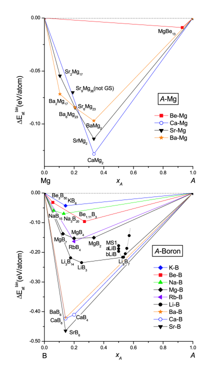
Figure 1: (Color online) Formation energies $\Delta E^{\texttt{\footnotesize bin}}_{\texttt{\footnotesize at}}$ for Mg-B, B-$A$, and Mg-$A$ binary ground states ($A$=Li, Be, Na, Mg, K, Ca, Rb, Sr, Cs, Ba) from Table 4. The dashed parabola for the Li-B system indicates the linear chains phases of Ref. Kolmogorov_Lithium_Borides,

The existence of the ground states for a given binary $A$-$B$ system is based on binary bulk formation energy, which, for each phase $\phi$ with stoichiometry $A_{x_{\texttt{\tiny A}}}B_{x_{\texttt{\tiny B}}}$, is determined with respect to pure $A$ and $B$ energies $E_{\texttt{\footnotesize at}}(A)$ and $E_{\texttt{\footnotesize at}}(B)$ as

$$\Delta E^{\texttt{\footnotesize bin}}_{\texttt{\footnotesize at}}(\phi)\equiv E_{\texttt{\footnotesize at}}(\phi)-x_{\texttt{\footnotesize A}}E_{\texttt{\footnotesize at}}(A)-x_{\texttt{\footnotesize B}}E_{\texttt{\footnotesize at}}(B).$$ (27)

The results are presented at Table 4 and in Figure 1. For each element $A$, the reference energy is chosen to be the lowest among the pure fcc, bcc and hcp energiesSC15 . The reference energy for boron is taken to be $\alpha$-boron (Refs. Pauling, ; aLiB, ; bLiB, ; boron, ; MS1, ).

All experimentally observed phases are confirmed except for Sr₉Mg₃₈ (P6₃/mmc). We also find two possible new phases, CaB₄ and RbB₄, both P4/mbm (#127) and with UB₄ prototype (CaB₄ was previously identified in ab initio online databaseCaB4 ). The formation energies for Ba₂Mg₁₇, Ba₆Mg₂₃, BaMg₂, and CaMg₂ are similar to those of Ref. ZKL07, (reported as -0.079 eV, -0.089 eV, -0.088 eV, and -0.126 eV, respectively). The small differences can be explained on the basis of different GGA pseudopotentials (PW91 versus PBE) and different energy cut-offs (414 eV versus 360 eV). Our results can not be compared with the thermodynamic discussion based on the semi-empirical Miedema method reported in Ref. WuGao05, , because we include further ground state prototypes other than those used in the heat of formations fitting in Ref. WuGao05, .

Figure 2: (color online) The ternary ground state phase diagrams of Mg-B-$A$ alloys ($A$=Li, Be, Na). The filled circles represent known ground states. The blue stars and red triangles represent the substitutional (Mg₇B${}_{56}A$, Mg₃B${}_{16}A$, Mg₇B${}_{16}A$) and interstitial (Mg₈B${}_{56}A$, Mg₄B${}_{16}A$, Mg₈B${}_{16}A$) supercells, respectively. Each supercell has been constructed from the most appropriate Mg-B compound (MgB₂, MgB₄, or MgB₇). The question mark in the Mg-B-Be system indicates the existence of new possible ternary ground state(s) (Sec. VI).

Figure 3: (color online) The ternary ground state phase diagrams of Mg-B-$A$ alloys ($A$=K, Rb, Cs).

Figure 4: (color online) The ternary ground state phase diagrams of Mg-B-$A$ alloys ($A$=Ca, Sr, Ba).

The calculated ternary ground state phase diagrams for Mg-B-$A$ alloys are depicted in Figs. 2,3,4. Note that in each phase diagram, the red triangles and blue stars represent the supercells with one interstitial or substitutional $A$ atom, respectively. In the interstitial case, the supercells belong to the lines Mg_nB_m$\leftrightarrow{A}$, while in the substitutional case, the supercells belong to the lines parallel to Mg$\leftrightarrow{A}$ and intersecting the Mg_nB_m (constant B concentration).

Formation energies numerical results

Table 5: Interstitial (i) and substitutional (s) quantities for alkali and alkaline earth solute elements $A$ in MgB₂, MgB₄, and MgB₇ compounds.: “raw” formation energies $\mu_{i}$, $\overline{\mu}_{s}$ (Eq. (1)), “true” formation energies $E_{\texttt{\footnotesize A}}^{(i)}$, $E_{\texttt{\footnotesize A}}^{(s)}$ (Eq. (2)) and low-solubility formation energies $E_{\texttt{\footnotesize sol}}^{(i)}$, $E_{\texttt{\footnotesize sol}}^{(s)}$ (Eqs. (3)). In each case, the presented value is the lowest one among all the possible interstitial or substitutional positions.

		MgB2		MgB4		MgB7
$A$	(eV)	(i)	(s)	(i)	(s)	(i)	(s)
Li	$\mu_{i},\overline{\mu}_{s}$	0.542	-0.111	0.234	-0.109	-0.959	-0.055
	$E_{\texttt{\footnotesize A}}^{(i,s)}$	2.444	0.310	2.136	0.312	0.943	0.366
	$E_{\texttt{\footnotesize sol}}^{(i,s)}$	2.716	0.574	2.654	0.686	1.657	0.506
Be	$\mu_{i},\overline{\mu}_{s}$	-2.665	-0.876	-0.506	-0.710	-1.577	-2.100
	$E_{\texttt{\footnotesize A}}^{(i,s)}$	1.042	1.350	3.201	1.516	2.130	0.126
	$E_{\texttt{\footnotesize sol}}^{(i,s)}$	1.054	1.21	3.201	1.256	2.181	-0.557
Na	$\mu_{i},\overline{\mu}_{s}$	5.623	1.839	2.409	1.285	1.999	0.869
	$E_{\texttt{\footnotesize A}}^{(i,s)}$	6.932	1.666	3.718	1.113	3.308	0.697
	$E_{\texttt{\footnotesize sol}}^{(i,s)}$	6.944	1.526	3.718	0.802	3.308	0.147
K	$\mu_{i},\overline{\mu}_{s}$	7.022	4.674	2.984	3.001	3.453	2.077
	$E_{\texttt{\footnotesize A}}^{(i,s)}$	8.061	4.232	4.023	2.559	4.492	1.635
	$E_{\texttt{\footnotesize sol}}^{(i,s)}$	8.073	4.092	4.023	2.248	4.492	0.838
Ca	$\mu_{i},\overline{\mu}_{s}$	2.833	-0.295	1.042	-1.107	1.251	-1.941
	$E_{\texttt{\footnotesize A}}^{(i,s)}$	4.751	-0.732	2.960	-0.671	3.169	-1.504
	$E_{\texttt{\footnotesize sol}}^{(i,s)}$	6.364	1.747	4.993	1.218	5.453	0.358
Rb	$\mu_{i},\overline{\mu}_{s}$	9.463	6.572	3.733	3.957	4.751	3.312
	$E_{\texttt{\footnotesize A}}^{(i,s)}$	10.393	6.021	4.663	3.406	5.681	2.761
	$E_{\texttt{\footnotesize sol}}^{(i,s)}$	10.406	5.981	4.862	3.460	6.047	2.477
Sr	$\mu_{i},\overline{\mu}_{s}$	5.514	1.761	1.334	0.221	2.149	-0.960
	$E_{\texttt{\footnotesize A}}^{(i,s)}$	7.138	1.618	2.958	0.364	3.773	-0.817
	$E_{\texttt{\footnotesize sol}}^{(i,s)}$	9.042	3.802	5.282	2.544	6.348	1.331
Cs	$\mu_{i},\overline{\mu}_{s}$	4.663	8.436	4.559	5.064	6.488	5.131
	$E_{\texttt{\footnotesize A}}^{(i,s)}$	5.523	7.815	5.419	4.444	7.349	4.510
	$E_{\texttt{\footnotesize sol}}^{(i,s)}$	5.536	7.675	5.419	4.134	7.349	3.411
Ba	$\mu_{i},\overline{\mu}_{s}$	2.450	3.959	1.365	1.084	3.118	0.335
	$E_{\texttt{\footnotesize A}}^{(i,s)}$	4.373	3.518	3.288	1.525	5.041	0.777
	$E_{\texttt{\footnotesize sol}}^{(i,s)}$	5.971	5.99	5.306	3.400	7.309	2.624

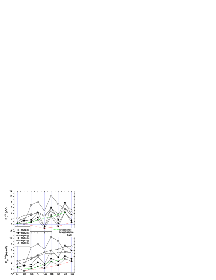
Figure 5: (Color online) Representation of the formations energies from Table 5. Dashed (green) and dotted (red) lines connect the lowest formation energies for alkali and alkaline earth elements, respectively.

The calculated parameters of the model (“raw” $\mu_{i}$, $\overline{\mu}_{s}$ (Eq. (1)), “true”- $E_{\texttt{\footnotesize A}}^{(i)}$, $E_{\texttt{\footnotesize A}}^{(s)}$ (Eq. (2)) and low-solubility $E_{\texttt{\footnotesize sol}}^{(i)}$, $E_{\texttt{\footnotesize sol}}^{(s)}$ (Eqs. (3)) formation energies) are presented in Table 5 and in Fig. 5.

The values of the low-solubility energies reported in Table 5 suggest the following. (a) Only $E_{\texttt{\footnotesize sol}}^{(s)}$ for substitutional Be in MgB₇ was found to be negative, indicating the existence of unknown ground state(s) within the triangle MgB${}_{7}\leftrightarrow{}$Be₃B${}_{50}\leftrightarrow{}$Be_1.11B₃. This fact is summarized by the question mark in Fig. 2. (b) Generally, the substitutional systems have lower formation energy than the interstitial systems. Exceptions are Be, Cs, and Ba in MgB₂; (c) Although oscillating, the formation energies tends to increase with the element number, as shown in Fig. 5. Regular oscillations are observed for all substitutionals systams starting with Na. The lower and higher boundaries of such correspond to alkaline earth and alkali elements, respectively. (d) Na, Ca, and Li substitutionals in MgB₇ have the lowest formation energies (0.147 eV, 0.358 eV, and 0.506 eV, respectively), resulting in high solubility (Sec. VII). (e) In general for substitutionals systems, the higher boron contents the lower formation energy (except Li and Be). (f) The corresponding “true” $E_{\texttt{\footnotesize A}}^{(i,s)}$ and low-solubility $E_{\texttt{\footnotesize sol}}^{(i,s)}(A)$ formation energies generally demonstrate a similar behavior as functions of $A$. Exceptions are $E_{\texttt{\footnotesize A}}^{(s)}<0$ for $A$=Ca and Sr and $E_{\texttt{\footnotesize sol}}^{(s)}(A)<0$ for $A$=Be. The difference is due to the consideration of all the known ground states for the determination of $E_{\texttt{\footnotesize sol}}^{(i,s)}$ and not only pure Mg, B and $A$ (as for $E_{\texttt{\footnotesize A}}^{(i,s)}$).

For Li-Mg-B, in Ref. BernMass06, the formation energies were obtained from first principles for interstitial and substitutional Li in boron-rich MgB₂ (3.00 eV and 0.27 eV, respectively). The results of Ref. BernMass06, are different form our low-solubility formation energies $E_{\texttt{\footnotesize sol}}^{(i)}$(Li)=2.72 eV and $E_{\texttt{\footnotesize sol}}^{(s)}$(Li)=0.57 eV (see Table 5), because only the hexagonal $\alpha$-LiB phase was considered as a ground state in Ref. BernMass06, and the other boron-rich phases were reported to be unstable (the $\alpha$-LiB was refined in Ref. Kolmogorov_Lithium_Borides, by variational minimization of the Li and B concentration as Li₈B₇). However, in our high-throughput framework, we found LiB₃ and Li₃B₁₄ to be stable LiBBB , and the approriate analysis of the formation energies should be done with respect to the triangle MgB₂$\leftrightarrow{}$LiB₃$\leftrightarrow{}$Mg as shown in Fig. 2. In the low-solubility limit of Li, since the supercell concentration is close to MgB₂, the lever rule of phase decomposition of the mixtures does not cause significant errors if the energies are calculated with respect to other references, and therefore the results of Ref. BernMass06, are somehow similar.

For Na-Mg-B, it can be shown that the substitutional Na formation energy in magnesium-rich MgB₂ (1.74 eV) obtained in Ref. BernMass06, is equivalent to our “true” formation energy for substitutional Na in MgB₂ ($E_{\texttt{\footnotesize Na}}^{(s)}=1.67$ eV, see Table 5). The observed small numerical difference between two results can be attributed to the different energy cutoffs for the basis set (414 eV versus 312 eV) note5 .

VII Solubility results

Solubility results are presented in Table 6 (the low-solubility approximation values are shown in brackets). We report only values larger than 10^-6 (Li, Na, Ca, and K). The values on Table 6 suggest the following. (a) Na is the only element which has a substantial solubility: Na in MgB₇ is $\sim$ 0.5-1 % at $T=650-1000$ K. (b) The substitutional solubility of Be in MgB₇ can not be determined because the corresponding formation energy $E_{\texttt{\footnotesize sol}}^{(s)}$ (see Eq. (3)) is negative implying that the ground state list is not complete. Thus the approach of Sec. V is not applicable. (c) In agreement with their lowest formation energies $E_{\texttt{\footnotesize sol}}^{(s)}$ (Table 5 and Fig. 5), substitutional Li, Na, and Ca experience the largest solubilities among all studied systems; (d) Due to their comsiderably high formation energies $E_{\texttt{\footnotesize sol}}^{(i)}$ (Table 5 and Fig. 5), all the investigated interstitial systems have negligible solubilities. (e) The low-solubility approximation and the general theory agree within 5%.

Table 6: Calculated equilibrium interstitial $x_{\texttt{\footnotesize A}^{(i)}}^{(1)}$ (i) and substitutional $x_{\texttt{\footnotesize A}^{(s)}}^{(1)}$ (s) $A$-solute concentrations at temperatures $T=$300, 650, and 1000 K, in MgB₂, MgB₄, and MgB₇ compounds. The values obtained within the low-solubility approximation are reported in brackets. Zeros are used for values smaller than $10^{-6}$. For Be “$\Delta E<0$” indicates that the corresponding formation energy $E_{\texttt{\footnotesize sol}}^{(s)}$ (see Eq. (3)) is negative implying that the ground state(s) list is not complete and the approach of Sec. V is not applicable.

$x_{\texttt{\footnotesize A}^{(i,s)}}^{(1)}$		MgB2		MgB4		MgB7
$A$	$T$ (K)	i	s	i	s	i	s
Li	300	0	0	0	0	0	0
	650	0	1.3$\times 10^{-5}$	0	0	0	9.9$\times 10^{-6}$
			(1.2$\times 10^{-5}$)				(9.9$\times 10^{-6}$)
	1000	0	4.5$\times 10^{-4}$	0	6.9$\times 10^{-5}$	0	2.6$\times 10^{-4}$
			(4.3$\times 10^{-4}$)		(7.0$\times 10^{-5}$)		(2.6$\times 10^{-4}$)
Be	300	0	0	0	0	0	$\Delta E<0$
	650	0	0	0	0	0	$\Delta E<0$
	1000	0	0	0	0	0	$\Delta E<0$
Na	300	0	0	0	0	0	2.1$\times 10^{-4}$
							(2.1$\times 10^{-4}$)
	650	0	0	0	0	0	4.4$\times 10^{-3}$
							(4.2$\times 10^{-3}$)
	1000	0	0	0	1.8$\times 10^{-5}$	0	1.0$\times 10^{-2}$
					(1.8$\times 10^{-5}$)		(0.96$\times 10^{-2}$)
K	300	0	0	0	0	0	0
	650	0	0	0	0	0	0
	1000	0	0	0	0	0	3.6$\times 10^{-6}$
Ca	300	0	0	0	0	0	0
	650	0	0	0	0	0	1.1$\times 10^{-4}$
							(1.0$\times 10^{-4}$)
	1000	0	0	0	0	0	1.0$\times 10^{-3}$
							(0.96$\times 10^{-3}$)
Rb	300	0	0	0	0	0	0
	650	0	0	0	0	0	0
	1000	0	0	0	0	0	0
Sr	300	0	0	0	0	0	0
	650	0	0	0	0	0	0
	1000	0	0	0	0	0	0
Cs	300	0	0	0	0	0	0
	650	0	0	0	0	0	0
	1000	0	0	0	0	0	0
Ba	300	0	0	0	0	0	0
	650	0	0	0	0	0	0
	1000	0	0	0	0	0	0

The calculated negligible solubilities of Be, Na, Ca in MgB₂ agree with previous experimental observationsZhang02CaLi ; Tamp03CaSr ; Cheng03Ca ; Toul02NaCa ; Agost07Na ; Feln01Be . We did not find any sign of nonvanishing solubilities of Rb, Cs and Ba in the MgB₂ alloy even at high annealing temperature in disagreement with the reported experimental data of Ref. Palnich07RbCsBa, . However, our negligible Rb and Cs solubility in bulk MgB₂ are in agreement with the experimental conclusion made in Ref. Singh08RbCs, where the author suggest that Rb and Cs dopants most likely segregate in grain boundaries.

The obtained low solubilities of Li and Sr in MgB₂ differ from experimental vales (solubility up to $30\%$ in Refs. Zhao01Li, ; Owens01Li, ; Cimb02Li, ; Zhang02CaLi, ; Tamp03CaSr, ; Karp08Li, ). This discrepancy can be attributed to segregation of Li and Sr in the grain boundaries as was concluded for Rb and Cs in Ref. Singh08RbCs, . In particular, the value of $E_{\texttt{\footnotesize sol}}^{(s)}$=3.8 eV for Sr is too large for non-negligiblle bulk solubility. For Li in MgB₂ the calculated formation energy $E_{\texttt{\footnotesize sol}}^{(s)}$=0.57 eV is not very large and it is the smallest among the investigated solutes in MgB₂. In Ref. BernMass06, , qualitative conclusions about high solubility of Li and low solubility of Na in MgB₂ were made based on a large difference between the corresponding formation energies. Our numerical results demonstrate that, despite much lower formation energy of Li in comparison with Na in MgB₂, the Li-solubility is still very low (Sec. VI).

It should be emphasized that our model is in thermodynamical equilibrium which can be difficult to reach at low temperatures and the experimental equilibrium solubility tends usually to be overestimated. In fact, the formation of metastable and/or unstable states which are subsequently frozen at low temperatures, can make solubility measurements very challenging. In such scenarios, the measured solubility may correspond to spinodal concentration rather then actual binodal concentration or simply characterize the frozen out of equilibrium solubility remaining from the initial specimen preparation at higher temperature. Besides, the segregation of defects into grain-boundaries, especially in multicrystalline samples prepared through non optimal cooling dramatically affect the amount of frozen defects and solutes.

Although in our study we did not perform an extensive search over the configurational space of ternary alloy, if a new ternary phases were present near MgB₂, the solute atoms would concentrate and nucleate such phases, and this may be misinterpreted as a high solubility in MgB₂ phase. Furthermore, a new equilibrium ternary phase would result in an increase of impurities formation energies and, correspondingly, in a decrease of solubility. Numerical approximations in the first-principles are not expected to affect the values of solubility: i.e. tipically for $\delta E_{\texttt{\footnotesize sol}}\sim 30$ meV/atom, $\delta x_{\texttt{\footnotesize A}}^{(1)}\sim 2\times 10^{-4}$. Lattice vibrations and solute-solute interactions are neglected because they are not expected to play important roles at low temperatures and low solute concentrations.

VIII Conclusions

In the present paper, we present an approach to study the solubilities in ternary alloys. The advantage of the approach is in taking into account all known ternary ground states rather than just pure solids. Based on the approach, we propose an analytical low-solubility approximation that can be used for high-throughput calculations of solubilities in alloys.

Combining the developed approach with first principle calculations, we have determined the formation energies and solubilities of alkali (Li, Na, K, Rb, Cs) and alkaline earth (Be, Ca, Sr, Ba) metals in the Mg-B system. It is found that the considered metals have low solubilities in the boron-rich Mg-B alloy. Substitutional Na, Ca, and Li experience the the largest solubilities, with Na in MgB₇ reaching 0.5-1% at $T=650-1000$ K. All the considered interstitial scenarios leed to negligible solubilities. The solubility of Be in MgB₇ can not be determined with our model because the corresponding low-solubility formation energy is negative implying that the existing ground states list must be augmented through a more extensive search over the configurational space.

We also present a high-throughput search of ground states in binary Mg-B, Mg-$A$, and B-$A$ alloys ($A$=Li, Be, Na, Mg, K, Ca, Rb, Sr, Cs, Ba). Ternary phase diagrams Mg-B-$A$ are constructed based on of the determined phases. Sr₉Mg₃₈ is not an equilibrium ground state despite its high temperature validations. Two new ground states CaB₄ and RbB₄ are found.

References

- (1) Electronic address: stefano@duke.edu
- (2) J. Nagamatsu, N. Nakagawa, T. Muranaka, Y. Zenitani, and J. Akimitsu, Nature (London) 410, 63 (2001).
- (3) F. J. Owens, Physica C 363, 202 (2001).
- (4) Y. G. Zhao, X. P. Zhang, P. T. Qiao, H. T. Zhang, S. L. Jia, B. S. Cao, M. H. Zhu, Z. H. Han, X. L. Wang, and B. L. Gu, Physica C 361, 91 (2001).
- (5) X. P. Zhang, Y. G. Zhao, P. T. Qiao, Z. S. Yin, S. L. Jia, B. S. Cao, M. H. Zhu, Z. H. Han, Y. H. Xiong, P. J. Li, and B. L. Gu, Journal of Superconductivity: Incorporating Novel Magnetism, 15, 159 (2002).
- (6) M. R. Cimberle, M. Novak, P. Manfrinetti, and A. Palenzona, Supercond. Sci. Technol. 15, 47 (2002).
- (7) J. Karpinski, N. D. Zhigadlo, S. Katrych, K. Rogacki, B. Batlogg, M. Tortello, and R. Puzniak, Phys. Rev. B 77, 214507 (2008).
- (8) P. Toulemonde, N. Musolino, H. L. Suo, and R. Flükiger Journal of Superconductivity: Incorporating Novel Magnetism 15, 613 (2002).
- (9) A. Agostino, M. Panetta, P. Volpe, M. Truccato, S. Cagliero, L. Gozzelino, R. Gerbaldo, G. Ghigo, F. Laviano, G. Lopardo, and B. Minetti, IEEE Transactions on Applied Superconductivity 17, 2774 (2007).
- (10) A. V. Palnichenko, O. M. Vyaselev and N. S. Sidorov, JETP Letters 86, 272 (2007).
- (11) R. K. Singh, Y. Shen, R. Gandikota, D. Wright, C. Carvalho, J. M. Rowell, and N. Newman, Supercond. Sci. Technol. 21, 025012 (2008).
- (12) I. Felner, Physica C 353, 11 (2001).
- (13) C. H. Cheng, Y. Zhao, X. T. Zhu, J. Nowotny, C. C. Sorrell, T. Finlayson, and H. Zhang, Physica C 386, 588 (2003).
- (14) A. Tampieri, G. Celotti, S. Sprio, and D. Rinaldi, International Journal of Modern Physics B 17, 438 (2003).
- (15) X. S. Wu and J. Gao, Physica C 418, 151 (2005).
- (16) A. R. Miedema, P. F. de Chatel, F. R. de Boer, Physica B & C 100, 1 (1980).
- (17) W. Toop, Trans. Met. 237, 738 (1965) .
- (18) F. Bernardini and S. Massidda, Europhys. Lett., 76, 491 (2006).
- (19) T. B. Massalski, Binary Alloy Phase Diagrams, 2nd ed. (ASM International, Materials Park, OH, 2003).
- (20) Pauling file: Inorganic Materials Database and Design System - Binaries Edition, edited by P. Villars (ASM International, Metals Park, OH, 2002).
- (21) S. Curtarolo, D. Morgan, and G. Ceder, Calphad 29, 163-211 (2005).
- (22) S. Curtarolo, Aflow: a computational software to calculate properties of materials in a high-throughput fashion. http://materials.pratt.duke.edu/aflow.html
- (23) Y. Mishin and D. Farkas, Phil. Mag. A 75, 169 (1997); Y. Mishin and C. Herzig, Acta Mater. 48, 589 (2000).
- (24) The bar at indicates that the quantity is not a chemical potential itself, as the number of particle is conserved.
- (25) R. V. Chepulskii and S. Curtarolo, “Calculation of solubility in titanium alloys from first-principles”, submitted to Acta Materialia (2009). http://arxiv.org/abs/0901.0200
- (26) M. A. Krivoglaz and A. A. Smirnov, The Theory of Order-Disorder in Alloys (Macdonald, London, 1964).
- (27) C. Wagner and W. Schottky, Z. Physik. Chem. B 11, 163 (1930).
- (28) In this method, the general composition plays just a supplementary role not effecting the results if necessarily belongs to the three-phase compositional triangle.
- (29) C. Sigli, L. Maenner, C. Sztur, and R. Shahni, in Proceedings of the 6th International Conference on Aluminum Alloys (ICAA-6), edited by T. Sato et al. (Japan Institute of Light Metals, 1998), Vol. 1, p. 87
- (30) In this case, the approximation (a) implies the neglection of in Eq. (15) and in the denominator of Eq. (10), respectively.
- (31) S. Curtarolo, D. Morgan, K. Persson, J. Rodgers, and G. Ceder, Phys. Rev. Lett. 91, 135503 (2003).
- (32) A. N. Kolmogorov and S. Curtarolo, Phys. Rev. B 73, 180501(R) (2006).
- (33) A. N. Kolmogorov and S. Curtarolo, Phys. Rev. B 74, 224507 (2006).
- (34) G. Kresse and J. Hafner, Phys. Rev. B 47, 558 (1993).
- (35) P. E. Blochl, Phys. Rev. B 50, 17953 (1994).
- (36) Y. Wang and J. P. Perdew, Phys. Rev. B bf 44, 13 298 (1991).
- (37) http://www.qhull.org/
- (38) The approximation implies that a true-ternary ground state does not exist or, if it exist, it is in a region of the phase diagram not relevant for solubility of in MgB2, MgB4 and MgB7.
- (39) International Tables for Crystallography, Vol. A, edited by T. Hahn (D. Reidel, Dordrecht, 1983).
- (40) G. Mair, R. Nesper, and H.G. von Schnering, Journal of Solid State Chemistry 75, 30 (1988).
- (41) G. Mair, H.G. von Schnering, M. Wörle, and R. Nesper, Zeitschrift für Anorganische und Allgemeine Chemie 625, 1207 (1999).
- (42) F. X. Zhang, F. F. Xu, and T. Tanaka, Journal of Solid State Chemistry 177, 3070 (2004).
- (43) J. Y. Chan, F. R. Fronczek, D. P. Young, J. F. DiTusa, and P. W. Adams, Journal of Solid State Chemistry 163, 385 (2002).
- (44) T. W. Baker, Acta Crystallographica 15, 175 (1962).
- (45) R. Naslain and J. S. Kasper, Journal of Solid State Chemistry 1, 150 (1970).
- (46) B. Albert and K. Hofmann, Zeitschrift für Anorganische und Allgemeine Chemie 625, 709 (1999).
- (47) A. Guette, M. Barret, R. Naslain, P. Hagenmuller, L. E. Tergenius, and T. Lundström, Journal of the Less-Common Metals 82, 325 (1981).
- (48) A. Guette, R. Naslain, and J. Galy, Comptes Rendus Hebdomadaires des Seances de l’Academie des Sciences, Serie C: Sciences Chimiques 275, 41 (1972).
- (49) N. V. Vekshina, L. Y. Markovskii, Y. D. Kondrashev, and T. K. Voevodskaya, Journal of Applied Chemistry of the USSR, translated from Zhurnal Prikladnoi Khimii 44, 970 (1971).
- (50) R. Naslain and J. Etourneau, Comptes Rendus Hebdomadaires des Seances de l’Academie des Sciences, Serie C: Sciences Chimiques 263, 484 (1966).
- (51) L. Pauling and S. Weinbaum, Zeitschrift für Kristallographie, Kristallgeometrie, Kristallphysik, Kristallchemie 87, 181 (1934).
- (52) M. Widom et. al., Alloy Database, http://alloy.phys.cmu.edu/.
- (53) H. Nowotny, Zeitschrift für Metallkunde 37, 31 (1946).
- (54) P. P. Blum and F. Bertaut, Acta Crystallographica 7, 81 (1954).
- (55) E. I. Gladyshevskii, P. I. Kripyakevich, M. Y. Teslyuk, O. S. Zarechnyuk, and Yu. B. Kuz’ma, Soviet Physics Crystallography, translated from Kristallografiya 6, 207 (1961).
- (56) F. E. Wang, F. A. Kanda, C. F. Miskell, and A. J. King, Acta Crystallographica 18, 24 (1965).
- (57) E. I. Gladyshevskii, P. I. Kripyakevich, Yu. B. Kuz’ma, and M. Y. Teslyuk, Soviet Physics Crystallography, translated from Kristallografiya 6, 615 (1961).
- (58) E. Hellner and F. Laves, Zeitschrift f r Kristallographie, Kristallgeometrie, Kristallphysik, Kristallchemie 105, 134 (1943).
- (59) Y. Wang, S. Curtarolo, C. Jiang, R. Arroyave, T. Wang, G. Ceder, L. Q. Chen, and Z. K. Liu, Calphad 28, 79-90 (2004).
- (60) Z. Liu, X. Qu, B. Huang, and Z. Li, J. Alloys Compd. 311, 256 (2000).
- (61) H. Rosner and W. E. Pickett, Phys. Rev. B 67, 054104 (2003).
- (62) M. Widom and M. Mihalkovic, Phys. Rev. B 77, 064113 (2008).
- (63) H. Zhang, J. Saal, A. Saengdeejing, Y. Wang, L.-Q. Chen and Z. K. Liu, in Magnesium Technology 2007, eds. R. S. Beals, A. A. Luo, N. R. Neelameggham and M. O. Pekguleryuz, Minerals, Metals and Materials Society/AIME, (Warrendale, PA, 2007), p. 345.
- (64) H. B. Borgstedt, and C. Guminsky, J. Phase Equilibria 24, 572 (2003).
- (65) As shown in Sec. V, the low-solubility formation energy (Na)=1.53 eV rather than “true” formation energy is more accurate for corresponding solubility characterization when the system is miscible. The 0.14 eV difference between and (Na) suggests that the effect of other ground state (MgB4, see Fig. 2) on the formation energy and subsequently on the solubility is not negligible.