Optimized L2-Orthogonal STC CPM for 3 Antennas

Abstract

In this paper, we introduce further our recently designed family of L² orthogonal Space-Time codes for CPM. With their advantage of maintaining both the constant envelope properties of CPM, the diversity of Space-Time codes and moreover orthogonality, and thus reduced decoding complexity, these codes are also full rate, even for more than two transmitting antennas.

The issue of power efficiency for these codes is first dealt with by proving that the inherent increase in bandwidth in these systems is quite moderate. It is then detailed how the initial state of the code influences the coding gain and has to be optimized. For the two and three antennas case, we determine the optimal values by computer simulations and show how the coding gain and therewith the bit error performance are significantly improved by this optimization.

I Introduction

The combination of space-time coding (STC) and continuous phase modulation (CPM) is an attractive field of research because the combination of STC and CPM brings the benefits of diversity and low power consumption to wireless communications. Zhang and Fitz [1] were the first to apply this idea by constructing a trellis based scheme. This idea was pursued by Zajić and Stüber in [2] for full response CPM, afterward optimized [3] and extended to partial response CPM in [4]. But for these codes the decoding effort grows exponentially with the number of transmitting antennas. This was circumvented by burst-wise orthogonality introduced by Silvester, Schober and Lampe in [5] and by block-wise orthogonality established by Wang and Xia [6][7]. Unfortunately, based on the Alamouti code [8], this latter design is restricted to two antennas. This restriction was partially circumvented in [9] by using quasi orthogonal STC for 4 transmitting antennas. However, to our knowledge, there was so far no consistent orthogonal design for a general number of antennas.

In our previous publications, by relaxing the orthogonality condition, we have been able to construct new $L^{2}$-orthogonal space-time codes which achieve full rate and full diversity with low decoding effort. More precisely, in [10] we have generalized the two-antenna code proposed by Wang and Xia [7] from pointwise to $L^{2}$-orthogonality and in [11] and [12], we introduce the first $L^{2}$-orthogonal code for CPM with three antennas. In this paper we shortly display some of these results and focus on several properties of these codes. Of special interest is the optimization of the bit error rate which depends on the initial phase of the system. Our simulation results illustrate the systemic behavior of these conditions.

II Parallel Coded CPM

II-A Space-Time code block

In MIMO systems, the signal sent $s(t)$ is transmitted via $L_{t}$ transmitting antennas. Here, similarly to [7], the continuous phase modulated sending signal will be split into blocks

$$\mathbf{S}(t)=\left[\begin{smallmatrix}s_{1,1}(t)&\ldots&s_{1,L_{t}}(t)\\ \vdots&s_{m,r}(t)&\vdots\\ s_{L_{t},1}(t)&\ldots&s_{L_{t},L_{t}}(t)\\ \end{smallmatrix}\right]$$ (1)

where each element of the sending matrix

$$s_{m,r}(t)=\sqrt{\frac{E_{s}}{L_{t}T}}\exp\left(j2\pi\phi_{m,r}(t)\right)$$ (2)

is defined within the time interval $(L_{t}l+r-1)T\leq t\leq(L_{t}l+r)T$. The indexes $m$ and $r$ denote respectively the sending antenna and the time slot in a block. $E_{s}$ is the symbol energy per transmit antenna Tx and per symbol time $T$. The phase signal

$$\phi_{m,r}(t)=\theta_{m}(L_{t}l+r)+h\sum_{i=1}^{\gamma}d_{m,r}^{(l,i)}q(t-i^{\prime}T)+c_{m,r}(t)$$ (3)

is essentially the phase of a conventional CPM signal [13] with an additional correction factor $c_{m,r}(t)$. The data symbols $d_{m,r}^{(l,i)}$ are uniquely determined for each element of the code block. A central point of the coding scheme is the mapping between these symbols and the data sequence $d_{j}$ with $d_{j}\in\Omega_{d}=\{-M+1,-M+3,\ldots,M-1\}$. As in conventional CPM, $h=2m_{0}/p$ is the modulation index where $m_{0}$ and $p$ are relative primes. The phase smoothing function $q(t)$ is a continuous function with $q(t)=0$ for $t\leq 0$ and $q(t)=1/2$ for $t\geq\gamma T$ and $\gamma$ is the memory length. The phase memory will be obtained from the definitions of correction factor and the mapping of the data symbols.

II-B $L^{2}-orthogonality$

To achieve simplified blockwise decoding as in systems based on orthogonal space-time block codes (OSTBC) [8][7], it is sufficient [11] to force each block to be $L^{2}$-orthogonal

$$\int\limits_{lL_{t}T}^{(l+1)L_{t}T}\mathbf{S}(t)\mathbf{S}^{\operatorname{\mathsf{H}}}(t)\operatorname{d\!}t=E_{s}\mathbf{I}$$ (4)

where $\mathbf{I}$ is the identity matrix. Hence the correlation between two different Tx antennas $s_{m,r}(t)$ and $s_{m^{\prime},r}(t)$ is zeroed over the $l^{\mbox{th}}$ complete STC block if

$$\int\limits_{lL_{t}T}^{(l+1)L_{t}T}s_{m,r}(t)s_{m^{\prime},r}^{*}(t)\operatorname{d\!}t=0$$ (5)

with $m\neq m^{\prime}$. Now, from theses conditions, $L^{2}$-orthogonal codes can be constructed [10][11][12] by expressing our design criteria:

1. the mapping of the data symbols $d_{m,r}^{(l,i)}$ to the data sequence $d_{j}$ and

2. the correction factor $c_{m,r}(t)$.

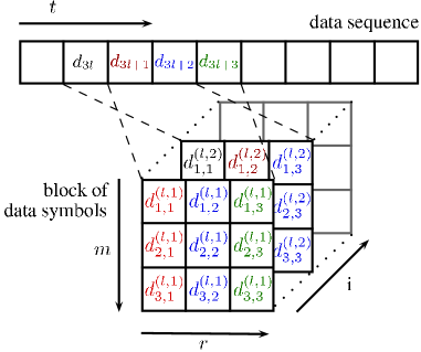
Figure 1: Mapping of the uncoded data sequence to the code block for 3 Tx antennas

Mapping: The most convenient mapping [11] is the parallel mapping where each data symbol of one time slot $r$ for $m=1,\ldots,L_{T}$ is mapped to the same symbol of the data sequence $d_{j}$. The following $L_{t}$ data symbols at $r+1$ are mapped to $d_{j+1}$ and so on. Each row of the code is therewith modulated by the same symbols of the data sequence and

$$d_{m,r}^{(l,i)}=d_{L_{t}l+r-i+1}$$ (6)

Due to this parallel structure, this solution is named parallel codes (PC). This mapping is illustrated in Figure 1.

Correction factor: The correction factor is determined by the phase difference $\Delta\phi$ between the different transmitting antennas at the end of each symbol in the code block. To ensure phase continuity, this difference has to be

• $1/2$ at $t=(2l+1)T$ for 2 Tx antennas

• and $1/3$ or $2/3$ at $t=(3l+1)T$ and $2/3$ or $4/3$ at $t=(3l+2)T$ for 3 Tx antennas.

We define the linear correction factor (linPC) as

$$c_{m,r}(t)=\frac{m-1}{L_{t}}\cdot\frac{t-(L_{t}l+r)T}{T}$$ (7)

and a more complex one based on the phase smoothing function $q(t)$ as

$$c_{m,r}(t)=\frac{m-1}{L_{t}}\sum\limits_{i=1}^{\gamma}2q(t-i^{\prime}T).$$ (8)

Without loss of generality, the correction factor of the first antenna is set to $c_{1,r}(t)=0$. Using Eq. (8) with Eq. (3) one can see that the sums from each equation can be merged. So, by combining the correction factor with the data symbol, we get new alphabets for each transmitting antenna $m$:

$$\textstyle\Omega_{d_{m}}=\{{\scriptstyle-M+1+\frac{2(m-1)}{L_{t}h},-M+3+\frac{2(m-1)}{L_{t}h},\ldots,M-1+\frac{2(m-1)}{L_{t}h}}\}.$$

Consequently, this code is called offset PC (offPC) and may be seen as $L_{t}$ conventional CPM signals with different alphabet sets $\Omega_{d_{m}}$ for each antenna $m$. The alphabet of the first antenna $\Omega_{d_{1}}$ is equal to the alphabet of a conventional CPM $\Omega_{d}$. For example, for two transmitting antennas we have $c_{1,r}(t)=0$, $c_{2,r}=\sum_{i=1}^{\gamma}q(t-i^{\prime}T)/2$ and then $\Omega_{d_{1}}=\Omega_{d}=\{-M+1,-M+3,\ldots,M-1\}$ and $\Omega_{d_{2}}=\{-M+1+1/h,-M+3+1/h,\ldots,M-1+1/h\}$. This intuitive representation greatly simplifies modulation and demodulation [11].

With these definitions of the coding scheme, we can rewrite the correction factor in the more generic form

$$\theta_{m}(L_{t}l+r+1)=\theta_{m}(L_{t}l+r)+\xi(L_{t}l+r)$$ (9)

where the function $\xi(L_{t}l+r)$ guarantees the continuity of the phase for any correction factor and mapping. For parallel mapping (similarly to conventional CPM) and $c_{m,r}(t)=0$, we get $\xi(L_{t}l+r)=\frac{h}{2}d_{L_{t}l+1-\gamma}$.

III Initial Phase

Our model includes now all the necessary parameters to construct $L^{2}$-orthogonal STC. The modulation index $h$ and the phase smoothing function $q(t)$ can be chosen with the usual restrictions of conventional CPM detailed above.

As proved by our simulations in section IV, the values of the initial phases $\theta_{m}(1)$, which are known to have no influence in conventional CPM systems [13], will be shown to have instead a great importance on the performance of the proposed code.

III-A Continuous-time Model

First, we need to introduce another formalism than the block structure used for design. The signals sent by each Tx antenna $m$ are rewritten as

$$\underline{s}_{m}(t)=\sqrt{\frac{E_{s}}{L_{t}T}}\exp(j2\pi[\theta_{m}(1)+h\sum\limits_{i=1}^{N_{c}}d_{i}q(t-(i-1)T)+c_{m}(t)]).$$ (10)

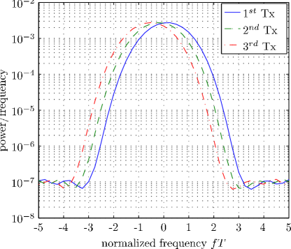
Figure 2: Power spectral density of the linPC analyzed with the Welch algorithm

In Eq. (10) the phase memory terms $\theta_{m}(L_{t}l+r)$ get included in the summation term. Only the initial phase $\theta_{m}(1)$ remains. This is due to the property of continuity in the definition of every symbol over the whole time $N_{c}T$ where $N_{c}$ is the number of transmitted symbols. As a result of the parallel mapping, the data symbols $d_{i}$ are also equal for each antenna. For offPC codes, we use the modified alphabets detailed in section II-B and no additional correction factor is necessary. For linPC codes, the correction factor $c_{m}(t)$ simplifies to a continuous linear function $c_{m}(t)=(m-1)t/L_{t}$.

It is interesting to see that for the second Tx antenna, the correction factor causes a constant phase offset of $2\pi/L_{t}$ per symbol and of $2\pi$ per block. For the 3 Tx antennas case, these offsets are multiplied by 2. The same effect is observed from the offset added to the alphabet $\Omega_{d_{m}}$.

This phase offset induces a frequency shift. For a phase shift of $2\pi(m-1)/L_{t}$ on a period of $T$, we get a frequency shift of $\Delta f_{m}=(m-1)/TL_{t}$ for antenna $m$ and a symbol length $T$.

Figure 2 shows the simulated power spectral density for the linPC code with 3 Tx antennas, $h=1/2$, $g=2$ and $M=4$. To achieve an attenuation in power of -30dB, a bandwidth expansion of some $5\,\mbox{Hz}T$ is necessary. This corresponds to an increased bandwidth demand of $\frac{\Delta f_{2}T}{5\mbox{Hz}T}=\frac{2}{3\cdot 5}=0.133$. As the alphabet size $M$ grows, the absolute bandwidth of the CPM signal widens but the shift caused by the coding scheme is constant. Therewith the additional relative bandwidth eventually decreases.

It should be recalled here that the highest achievable rate for linear codes with 4 Tx antennas is 3/4 [14]. It means that to transmit the same quantity of data during the same duration of time as for our proposed code a 25% increase in bandwidth is necessary.

With this continuous-time formalism, the signals sent can be rewritten in vector form as $\underline{s}(t)=[\underline{s}_{1}(t),\underline{s}_{2}(t),\cdots,\underline{s}_{L_{t}}(t)]^{\operatorname{\mathsf{T}}}$. Below underlined variables denote the vector representation and non-underlined variables the previously used matrix form. Thus we can write $\underline{s}(t)$ as the product of two matrices $\underline{\Theta}$ and $\underline{C}(t)$ and a vector $\underline{d}(t)$

$$\underline{s}(t)=\sqrt{\frac{E_{s}}{L_{t}T}}~{}\underline{\Theta}\,\underline{C}(t)\,\underline{d}(t)$$ (11)

The matrix of initial values $\underline{\Theta}=\operatorname{diag}(\underline{\theta})$ and the matrix of correction factors $\underline{C}(t)=\operatorname{diag}(\underline{c}(t))$ are $L_{t}\times L_{t}$ diagonal matrices obtained from the vectors

$$\underline{\theta}= \begin{bmatrix}\exp(j2\pi\theta_{1}(1))\\ \exp(j2\pi\theta_{2}(1))\\ \vdots\\ \exp(j2\pi\theta_{L_{t}}(1))\\ \end{bmatrix}, \underline{c}(t)= \begin{bmatrix}\exp(j2\pi c_{1}(t))\\ \exp(j2\pi c_{2}(1))\\ \vdots\\ \exp(j2\pi c_{L_{t}}(1))\\ \end{bmatrix}.$$ (12)

As a result of the parallel mapping, the vector of data symbols can be written as

$$\underline{d}(t)=\exp(j2\pi h\sum\limits_{i=1}^{N_{c}}d_{i}q(t-(i-1)T)){\begin{bmatrix}1&1&\ldots&1\end{bmatrix}}^{\operatorname{\mathsf{H}}}.$$ (13)

III-B Code Performance

The performance of theses codes may now by evaluated using the classical pair-wise error probability (PWEP). We assume optimal demodulation, i.e. maximum likelihood (ML) sequence detection (MLSD). Furthermore, it is considered that for $0\leq t\leq N_{c}T$ the signal $\underline{s}(t)$ modulated by the data sequence $d_{j}$ is the one truly sent. The PWEP is then the probability that this signal is erroneously detected as signal $\hat{\underline{s}}(t)$ modulated by $\hat{d}_{j}$ [2].

$$PWEP=P(\underline{s}(t)\rightarrow\hat{\underline{s}}(t)|\mathbf{A})=Q\left(\frac{\|\mathbf{A}^{\operatorname{\mathsf{T}}}\mathbf{\Delta}(t)\|}{\sqrt{2N_{0}}}\right)$$ (14)

where $\mathbf{A}$ is the channel matrix which is assumed to to have frequency flat quasi-static Rayleigh fading and mutual independent elements. The energy of noise is given by $N_{0}$ and $Q(\cdot)$ is the cumulative distribution function of the normal distribution (Q-function). The normalized difference vector $\mathbf{\Delta}(t)$ is given by

$$\mathbf{\Delta}(t)=\begin{bmatrix}\Delta_{1}(t)\\ \Delta_{2}(t)\\ \vdots\\ \Delta_{L_{t}}(t)\end{bmatrix}=\sqrt{\frac{L_{t}T}{E_{s}}}\begin{bmatrix}\underline{s}_{1}(t)-\hat{\underline{s}}_{1}(t)\\ \underline{s}_{2}(t)-\hat{\underline{s}}_{2}(t)\\ \vdots\\ \underline{s}_{L_{t}}(t)-\hat{\underline{s}}_{L_{t}}(t)\end{bmatrix}$$ (15)

The PWEP is minimized by maximizing the product of the eigenvalues of the signal matrix [15, 2]

$$\mathbf{C}_{s}=\left[\begin{smallmatrix}\int\limits_{0}^{N_{c}T}|\Delta_{1}(t)|^{2}\operatorname{d\!}t&\int\limits_{0}^{N_{c}T}\Delta_{1}(t)\Delta_{2}^{*}(t)\operatorname{d\!}t&\cdots&\int\limits_{0}^{N_{c}T}\Delta_{1}(t)\Delta_{L_{t}}^{*}(t)\operatorname{d\!}t\\ \int\limits_{0}^{N_{c}T}\Delta_{2}(t)\Delta_{1}^{*}(t)\operatorname{d\!}t&\int\limits_{0}^{N_{c}T}|\Delta_{2}(t)|^{2}\operatorname{d\!}t&\cdots&\int\limits_{0}^{N_{c}T}\Delta_{2}(t)\Delta_{L_{t}}^{*}(t)\operatorname{d\!}t\\ \vdots&&&\vdots\\ \int\limits_{0}^{N_{c}T}\Delta_{L_{t}}(t)\Delta_{1}^{*}(t)\operatorname{d\!}t&\int\limits_{0}^{N_{c}T}\Delta_{L_{t}}(t)\Delta_{2}^{*}(t)\operatorname{d\!}t&\cdots&\int\limits_{0}^{N_{c}T}|\Delta_{L_{t}}(t)|^{2}\operatorname{d\!}t\\ \end{smallmatrix}\right]$$ (16)

Using Eq. (11) and (15) the signal matrix can be written as

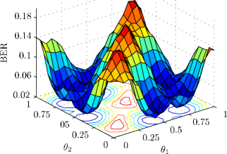
(a) offset PC with REC

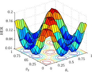
(b) offset PC with RC

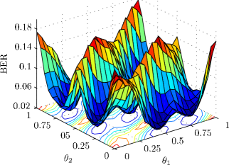
(c) linear PC with REC

Figure 3: Simulated BER for varying initial phase $\theta_{1}(1)$ and $\theta_{2}(1)$ and $\theta_{3}(1)=0$ for 3 Tx antennas at 13dB SNR

$$\mathbf{C}_{s}= \int\limits_{0}^{N_{c}T}\!\mathbf{\Delta}(t)\mathbf{\Delta}^{\operatorname{\mathsf{H}}}(t)\operatorname{d\!}t$$

$$= \int\limits_{0}^{N_{c}T}\!{\big{[}\underline{\Theta}\,\underline{C}(t)(\underline{d}(t)-\hat{\underline{d}}(t))\big{]}}\big{[}\underline{\Theta}\,\underline{C}(t)(\underline{d}(t)-\hat{\underline{d}}(t))\big{]}^{\operatorname{\mathsf{H}}}\operatorname{d\!}t$$

$$= ~{}\underline{\Theta}\big{(}\!\!\int\limits_{0}^{N_{c}T}\!\underline{C}(t)\,\Delta\underline{d}(t)\,\Delta\underline{d}^{\operatorname{\mathsf{H}}}(t)\,\underline{C}^{\operatorname{\mathsf{H}}}(t)\operatorname{d\!}t\big{)}\underline{\Theta}^{\operatorname{\mathsf{H}}}$$ (17)

with $\Delta\underline{d}(t)=\underline{d}(t)-\hat{\underline{d}}(t)$ and the integral over the matrix acting element-wise. Since $\underline{d}(t)$ has equal elements and is multiplied by its Hermitian transpose, we get an $L_{t}\times L_{t}$ all-ones matrix. This matrix is multiplied with the matrices of the correction factor and we obtain the correlation matrix of the correction vector

$$\mathbf{C}_{s}=\underline{\Theta}\!\int\limits_{0}^{N_{c}T}\!\underline{c}(t)\underline{c}^{\operatorname{\mathsf{H}}}(t)\operatorname{d\!}t~{}\underline{\Theta}^{\operatorname{\mathsf{H}}}.$$ (18)

By writing $c_{m}(t)=\frac{m-1}{L_{r}}\bar{c}(t)$ in Eq. (7) and (8), we get

$$\underline{c}_{m}(t)\underline{c}^{*}_{m^{\prime}}(t)=\exp\big{(}j2\pi\bar{c}(t)({\textstyle\frac{m-1}{L_{t}}-\frac{m^{\prime}-1}{L_{t}}})\big{)}.$$ (19)

The autocorrelation $\underline{c}_{m}(t)\underline{c}_{m}^{*}(t)$ is therewith always one and we have

$$\underline{c}(t)\underline{c}^{\operatorname{\mathsf{H}}}(t)=\left[\begin{smallmatrix}\exp\!\big{(}\frac{0}{L_{t}}j2\pi\bar{c}(t)\big{)}&\exp\!\big{(}-\frac{1}{L_{t}}j2\pi\bar{c}(t)\big{)}&\ldots&\exp\!\big{(}-\frac{L_{t}-1}{L_{t}}j2\pi\bar{c}(t)\big{)}\!\\ \exp\!\big{(}\frac{1}{L_{t}}j2\pi\bar{c}(t)\big{)}&\exp\!\big{(}\frac{0}{L_{t}}j2\pi\bar{c}(t)\big{)}&\ldots&\exp\!\big{(}-\frac{L_{t}-2}{L_{t}}j2\pi\bar{c}(t)\big{)}\!\\ \vdots&&&\vdots\\ \!\exp\!\big{(}\frac{L_{t}-1}{L_{t}}j2\pi\bar{c}(t)\big{)}&\exp\!\big{(}\frac{L_{t}-2}{L_{t}}j2\pi\bar{c}(t)\big{)}&\ldots&\exp\!\big{(}\frac{0}{L_{t}}j2\pi\bar{c}(t)\big{)}\\ \end{smallmatrix}\right]$$ (20)

The elementwise integration of this matrix is easily computed [12] in the special cases where $\bar{c}(t)$ is a linear function (linPC codes) or a sum of raised cosines (OffPC codes) [12]. In both cases, the matrix $\mathbf{C}_{s}$ is shown to have full rank [11] and thus our codes achieve full diversity. However, the PWEP approach doesn’t provide here any valuable estimate of the coding gain. For that reason, we detail hereafter some statistical estimates to show the influence of the initial phase values upon the coding gain.

IV Simulations

In this section, we benchmark by simulations the performance of the proposed codes. In all the simulations, we used an alphabet size of $M=4$ with 2-bit Gray-coding, a modulation index of $h=1/2$, a memory length of $\gamma=2$ and 12 samples per symbol. The signal is disturbed by complex code-block-wise Rayleigh fading of variance one. In this section all given phase values are relative values, e.g. 1 corresponds to $2\pi$ or $360^{\circ}$.

IV-A Two transmit antennas

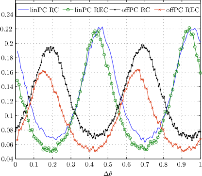
Figure 4: simulated BER for varying initial phase $\theta_{2}$ for 2 Tx antennas at SNR=12.5dB

The bit error rate (BER - $E_{b}/N_{0}$) for the proposed two transmitting antenna codes depends on the difference of the initial phase $\Delta\theta=\theta_{2}(1)-\theta_{1}(1)$. Figure 4 shows the results of computer simulations for linPC and offPC codes with different phase smoothing functions $q(t)$. The variation of performance covers almost one decade. This shows the importance of a carefully chosen initial phase.

Mainly, the position of the minimal BER seems to depend on the correction factor used. Between linPC and offPC, the minima are shifted by $1/4$. However, the phase smoothing function used has only minor influence on the position of the minima. It is also interesting to see that the distance between the minima is $1/2$ and further simulations show a periodicity of $1$.

IV-B Three transmit antennas

offPC	$\theta_{1}$	0.1	0.15	0.4	0.45	0.75	0.8
	$\theta_{2}$	0.45	0.75	0.8	0.1	0.15	0.4
linPC	$\theta_{1}$	0.75	0.4	0.45	0.7	0.05	0.1
	$\theta_{2}$	0.15	0.15	0.5	0.8	0.5	0.8

TABLE I: Initial phase values for minimal BER (SNR=12.5dB; 2REC)

For the three antennas codes, the BER also depends on the initial phase $\theta_{m}(1)$. Fig. 3 shows the simulation results for different codes with varying initial phases for the first and second antenna and null initial phase for the third antenna. It can be seen that the phase offset for a minimal BER depends on the correction factor chosen (Fig. 3(a) and 3(c)). However, similarly to the two antenna code, the form of the phase smoothing function $q(t)$ has almost no influence on the position of the minima (Fig. 3(a) and 3(b)). In Table I the optimal initial phase are summarized for the first and second antenna. Other simulations for different alphabet sizes $M$, modulation indexes $h$ and memory length $\gamma$ validate the position of the minima and prove it is an important issue for the optimal design of parallel codes.

IV-C Bit Error Rate

Fig. 5 shows the influence of Rayleigh fading channels on a CPM transmitter with a different number of antennas.

For the optimal two antenna system we used in the optimal case a frequency offset of $\Delta\theta=0.19$ for linPC and of $\Delta\theta=0.4$ for offPC. For the optimal three-antennas-codes, we took the following values from Fig. 3:

• offPC: $\theta_{1}(1)=0.1$, $\theta_{2}(1)=0.45$;

• linPC: $\theta_{1}(1)=0.4$, $\theta_{2}(1)=0.15$.

The non-optimal codes have no phase offset ($\theta_{1}(1)=\theta_{2}(1)=\Delta\theta=0$).

The optimized codes achieve the expected performance gain. For high SNR the BER decreases with 5dB/dec similar to a two antenna system with full diversity. The three Tx antennas code achieves a decay of some 3.5dB/dec. This validates the property of full diversity.

Fig. 5 shows clearly the improvement of the coding gain by using an optimized initial phase. Comparing the optimized codes with the non-optimal ones, we achieve an additional coding gain of around 5dB for the two antenna system and of around 7dB for the three Tx antennas.

Figure 5: BER for Rayleigh-fading channel

V Conclusion

In this paper, we detail the construction and analyze some of the properties of L2-orthogonal STC-CPM for two and three transmitting antennas. These codes are attractive due to their low-effort-decoding and the few restrictions the code-family set upon the parameters of CPM. We give a general formulation for two and three antenna parallel codes and introduce a continuous-time representation of the CPM signals. With this representation we are able to analyze how the coding gain depends on the initial phase of the system. Furthermore, we give the optimal values for the initial states obtained from computer simulation. The significant gain in performance for typical Rayleigh fading channels is shown and compared with non-optimal parallel codes.

References

- [1] X. Zhang and M. P. Fitz, “Space-time coding for Rayleigh fading channels in CPM system,” in Proc. of Annu. Allerton Conf. Communication, Control, and Computing, 2000.
- [2] A. Zajić and G. Stüber, “Continuous phase modulated space-time codes,” in Proc. of IEEE International Symposium on Communication Theory and Applications (ISCTA’05), July 2005, pp. 292 – 297.
- [3] ——, “Optimization of coding gain for full-response CPM space-time codes,” in Proc. of IEEE Global Telecommunications Conference (GLOBECOM ’06), Nov. 2006, pp. 1 – 5.
- [4] ——, “A space-time code design for partial-response CPM: Diversity order and coding gain,” in Proc. of IEEE International Conference on Communications (ICC’07), June 2007, pp. 719 – 724.
- [5] A. Silvester, R. Schober, and L. Lampe, “Burst-based orthogonal ST block coding for CPM,” IEEE Trans. Wireless Commun., vol. 6, pp. 1208 – 1212, April 2007.
- [6] G. Wang and X.-G. Xia, “An orthogonal space–time coded CPM system with fast decoding for two transmit antennas,” IEEE Trans. Inf. Theory, vol. 50, no. 3, pp. 486 – 493, March 2004.
- [7] D. Wang, G. Wang, and X.-G. Xia, “An orthogonal space–time coded partial response CPM system with fast decoding for two transmit antennas,” IEEE Trans. Wireless Commun., vol. 4, no. 5, pp. 2410 – 2422, Sept. 2005.
- [8] S. M. Alamouti, “A simple transmit diversity technique for wireless communications,” IEEE J. Sel. Areas Commun., vol. 16, no. 8, pp. 1451 – 1458, Oct. 1998.
- [9] G. Wang, W. Su, and X.-G. Xia, “Orthogonal-like space-time coded CPM system with fast decoding for three and four transmit antennas,” in Proc. of IEEE Global Telecommunications Conference (GLOBECOM ’03), Nov. 2003, pp. 3321 – 3325.
- [10] M. Hesse, J. Lebrun, and L. Deneire, “L2 orthogonal space time code for continuous phase modulation,” in Proc. of IEEE Workshop on Signal Processing Advances in Wireless Communications (SPAWC’08), July 2008, pp. 401 – 405.
- [11] ——, “L2 OSTC-CPM: Theory and design,” CNRS/University of Nice, Sophia Antipolis, Tech. Rep. I3S/RR-2008-03, 2008. [Online]. Available: http://arxiv.org/abs/0806.2760
- [12] ——, “Full rate L2-orthogonal space-time CPM for three antennas,” in Proc. of IEEE Global Telecommunications Conference (GLOBECOM ’08), accepted for publication., New Orleans, USA, 2008.
- [13] J. Anderson, T. Aulin, and C.-E. Sundberg, Digital Phase Modulation. Plenum Press, 1986.
- [14] V. Tarokh, H. Jafarkhani, and A. R. Calderbank, “Space–time block codes from orthogonal designs,” IEEE Trans. Inf. Theory, vol. 45, no. 5, pp. 1456 – 1567, July 1999.
- [15] X. Zhang and M. P. Fitz, “Space-time code design with continuous phase modulation,” IEEE J. Sel. Areas Commun., vol. 21, pp. 783 – 792, June 2003.