CONFORMATIONAL TRANSITIONS IN
MOLECULAR SYSTEMS

Abstract

Proteins are the “work horses” in biological systems. In almost all functions specific proteins are involved. They control molecular transport processes, stabilize the cell structure, enzymatically catalyze chemical reactions; others act as molecular motors in the complex machinery of molecular synthetization processes. Due to their significance, misfolds and malfunctions of proteins typically entail disastrous diseases, such as Alzheimer’s disease and bovine spongiform encephalopathy (BSE). Therefore, the understanding of the trinity of amino acid composition, geometric structure, and biological function is one of the most essential challenges for the natural sciences. Here, we glance at conformational transitions accompanying the structure formation in protein folding processes.

1 Conformational Mechanics of Proteins

Structural changes of polymers and, in particular, proteins in collapse and crystallization processes, but also in cluster formation and adsorption to substrates, require typically collective and cooperative rearrangements of chain segments or monomers. Structure formation is essential in biosystems as in many cases the function of a bioprotein is connected with its three-dimensional shape (the so-called “native fold”). Proteins are linear chains of amino acids linked by a peptide bond (see Fig. 1). Twenty different amino acids occur in biologically relevant, i.e., functional proteins. The amino acid residues differ in physical (e.g., electrostatic) and chemical (e.g., hydrophobic) properties. Hence, the sequence of amino acids typically entails a unique heterogeneity in geometric structure and, thus, a nonredundant biological function.

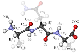
Figure 1: Atomic composition of the protein backbone. Amino acids are connected by the peptide bond between C${}^{\prime}_{i-1}$ and N_i. Side chains or amino acid residues (“res”) are usually connected to the backbone by a bond with the C${}^{\alpha}_{i}$ atom (except proline which has a second covalent bond to its backbone nitrogen).

Proteins are synthesized by the ribosomes in the cell, where the genetic code in the DNA is translated into a sequence of amino acids. The folding of a synthesized protein into its three-dimensional structure is frequently a spontaneous process. In a complex biological system, the large variety of processes which are necessary to keep an organism alive requires a large number of different functional proteins. In the human body, for example, about 100 000 different proteins fulfil specific functions. However, this number is extremely small, compared to the huge number of possible amino acid sequences ($=20^{N}$, where $N$ is the chain length and is typically between 100 and 3000). The reason is that bioproteins have to obey very specific requirements. Most important are stability, uniqueness, and functionality.

Under physiological conditions, flexible protein degrees of freedom are the dihedral angles, i.e., a subset of backbone and side-chain torsional angles (see Fig. 2). Denoting the set of dihedral angles of the $n$th amino acid in the chain by $\boldsymbol{\xi}_{n}=\{\phi_{n},\psi_{n},\omega_{n},\chi^{(1)}_{n},\chi^{(2)}_{n},\ldots\}$, the conformation of an $N$ residue protein is then entirely defined by ${\bf X}={\bf X}(\boldsymbol{\xi}_{1},\boldsymbol{\xi}_{2},\ldots,\boldsymbol{\xi}_{N})$. Therefore, the partition function can formally be written as a path integral over all possible conformations:

$$Z=\int{\cal D}{\bf X}\exp\left[-E({\bf X})/k_{B}T\right],\quad\int{\cal D}{\bf X}=\prod\limits_{n=1}^{N}\left[\int d\boldsymbol{\xi}_{n}\right],$$ (1)

where $E(\bf X)$ is the energy of the conformation $\bf X$ in a typically semiclassical all-atom protein model. A precise modeling is intricate because of the importance of quantum effects in this complex macromolecular system, which are “hidden” in the parametrization of the semiclassical model. Another important problem is the modeling of the surrounding, strongly polar solvent. The hydrophobic effect that causes the formation of a compact core of hydrophobic amino acids screened from the polar solvent by a shell of polar residues is expected to be the principal driving force towards the native, functional protein conformation. [3, 4, 5] Conformational transitions accompanying molecular structuring processes, however, exhibit similarities to thermodynamic phase transitions and it should thus be possible to characterize these transitions by means of a strongly reduced set of effective degrees of freedom, in close correspondence to order parameters that separate thermodynamic phases. Assuming that a single “order” parameter $Q$ is sufficient to distinguish between two (pseudo)phases, its mean value $\langle Q\rangle=Z^{-1}\int{\cal D}{\bf X}\,Q({\bf X})\exp\left[-E({\bf X})/k_{B}T\right]$ should possess significantly different values in these phases. In typical first-order-like nucleation transitions such as helix formation [1] or tertiary two-state folding [2], the free-energy landscape $F(Q)\sim-k_{B}T\ln\left\langle\delta(Q-Q_{0}({\bf X}))\right\rangle$ exhibits a single folding barrier.

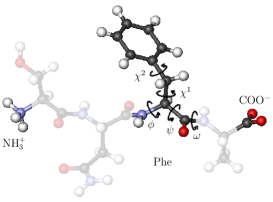
Figure 2: Definition of the backbone dihedral angles $\phi$, $\psi$, and $\omega$. Exemplified for phenylalanine, also the only two side-chain degrees of freedom $\chi^{1}$ and $\chi^{2}$ are denoted. The convention is that the torsional angles can have values between $-180^{\circ}$ and $+180^{\circ}$, counted from the N-terminus (NH${}_{3}^{+}$) to the C-terminus (COO^-) according to the right-hand rule and in the side chains starting from the C^α atom.

2 From Microscopic to Mesoscopic Modeling

If the characterization of conformational macrostates by low-dimensional parameter spaces is possible, it should also be apparent to introduce coarse-grained substructures and thus to reduce the complexity of the model to a minimum. Such minimal models for proteins have indeed been introduced [3, 4] and have proven useful in thermodynamic analyses of folding, adsorption, and aggregation of polymers and proteins. [5, 6, 7, 8, 2]

In the simplest approaches [3, 4], only two types of amino acids are considered: hydrophobic and polar residues. This is plausible as most of the 20 amino acids occurring in natural bioproteins can be classified with respect to their hydrophobicity. Amino acids with charged side chains or with residues containing polar groups (amide or hydroxylic) are soluble in the aqueous environment, because these groups are capable of forming hydrogen bonds with water molecules. Nonpolar amino acids do not form hydrogen bonds and, if exposed to water, would disturb the hydrogen-bond network. This is energetically unfavorable. In fact, hydrophobic amino acids effectively attract each other and typically form a compact hydrophobic core in the interior of the protein.

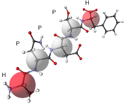
Figure 3: Coarse-graining proteins in a “united atom” approach. Each amino acid is contracted to a single “C^α” interaction point. The effective distance between adjacent, bonded interaction sites is about 3.8 Å. In the class of so-called hydrophobic-polar models, only hydrophobic (H) and polar (P) amino acid residues are distinguished.

Figure 3 shows an example how the complexity of a protein segment can be reduced by coarse-graining. On one hand, the residual complexity is limited by only distinguishing hydrophobic (H) and polar (P) amino acids. On the other hand, the steric extension of the side chains is mesoscopically rescaled and the whole side chain is contracted into a single interaction point. Volume exclusion in the interaction of different side chains is then energetically modeled by short-range repulsion. For this reason, lattice proteins are modeled as self-avoiding walks [3] and in off-lattice models Lennard-Jones-like potentials [4] satisfy this constraint.

Systematic enumeration studies of simplified hydrophobic-polar lattice models have indeed qualitatively revealed characteristic features of real proteins, such as the small number of amino acid sequences possessing a unique native fold, but also the comparatively small number of native topologies proteins fold into. [9] It is also remarkable that typical protein folding paths known from nature are also identified by employing coarse-grained models. This regards, in particular, folding landscapes with characteristic barriers – from the simple two-state characteristics with a single kinetic barrier, [2] over folding across several barriers via weakly stable intermediate structures, to folding into degenerate native states. [6] Metastable conformations as in the latter case are important for biological functions, where the local refolding of protein segments is essential, as, e.g., in molecular motors.

3 A Particularly Simple Example: Two-State Folding

A few years ago, experimental evidence was found that classes of proteins show particular simple folding characteristics, single exponential and two-state folding [10]. In the two-state folding process, the peptide is either in an unfolded, denatured state or it possesses a native-like, folded structure. In contrast to the barrier-free single-exponential folding, there exists an unstable transition state to be passed in the two-state folding process. This can nicely be seen in the exemplified chevron plot shown in Fig. 4, obtained from Monte Carlo computer simulations of folding and unfolding events of a mesoscopic protein model. [2] In this plot, the mean first passage (MFP) time $\tau_{\text{MFP}}$ (in Monte Carlo steps) is plotted versus temperature. The MFP time is obtained by averaging the times passed in the folding process from a random conformation to the stable fold over many folding trajectories. MFT times for unfolding events can be estimated in a like manner, but one starts from the native conformation and waits until the protein has unfolded. A structure is defined to be folded, if it is structurally close to the native conformation. A frequently used measure is the fraction $Q$ of already established native contacts (i.e., the number of residue pairs that reside within the optimal van der Waals distance), compared to the total number of contacts the native fold possesses. Thus, if $Q>0.5$, the structure is folded and unfolded if $Q<0.5$. For $Q=0.5$, the conformation is in the transition state. Apparently, $Q$ serves as a sort of order parameter.

The two branches in Fig. 4 belong to the folding and unfolding events. With increasing temperature folding times grow, and unfolding is getting slower with decreasing temperature. These two processes are in competition with each other and the intersection point defines the folding transition temperature. The whole process exhibits characteristics of first-order-like phase transitions. At the intersection point, the ensembles of folded and unfolded conformations coexist with equal weight. In the transition region, both branches exhibit exponential behavior. Thus, $\tau_{\text{MFP}}$ is directly related to exponential folding and unfolding rates $k_{f,u}\approx 1/\tau_{\text{MFP}}^{f,u}\sim\exp(-\varepsilon_{f,u}/k_{B}T)$, respectively, where the constants $\varepsilon_{f,u}$ determine the kinetic folding (unfolding) propensities. The dashed lines in Fig. 4 are tangents to the logarithmic folding and unfolding curves at the transition state temperature.

Figure 4: Chevron plot of the mean-first passage times from folding ($\bullet$) and unfolding ($\circ$) events at different temperatures. The hypothetic intersection point corresponds to the transition state. [2]

4 Conclusion

Conformational transitions of macromolecular systems, in particular, proteins, exhibit clear analogies to phase transitions in thermodynamics. The main difference is that proteins are finite systems and a thermodynamic limit does not exist. Nonetheless, the analysis of structure formation processes in terms of an “order” parameter is also a very useful approach to a better understanding of conformational transitions. In this context it also turns out to be reasonable to introduce coarse-grained models where the reduction to only relevant degrees of freedom allows for a more systematic analysis of characteristic features of protein folding processes than it is typically possible with models containing specific properties of all atoms.

References

- [1] G. Gökoğlu, M. Bachmann, T. Çelik, and W. Janke, Phys. Rev. E 74, 041802 (2006).
- [2] A. Kallias, M. Bachmann, and W. Janke, J. Chem. Phys. 128, 055102 (2008).
- [3] K. F. Lau and K. A. Dill, Macromolecules 22, 3986 (1989).
- [4] F. H. Stillinger and T. Head-Gordon, Phys. Rev. E 52, 2872 (1995).
- [5] M. Bachmann and W. Janke, Lect. Notes Phys. 736, 203 (2008).
- [6] S. Schnabel, M. Bachmann, and W. Janke, Phys. Rev. Lett. 98, 048103 (2007); J. Chem. Phys. 126, 105102 (2007).
- [7] M. Bachmann and W. Janke, Phys. Rev. Lett. 95, 058102 (2005); Phys. Rev. E 73, 041802 (2006); Phys. Rev. E 73, 020901(R) (2006).
- [8] C. Junghans, M. Bachmann, and W. Janke, Phys. Rev. Lett. 97, 218103 (2006); J. Chem. Phys. 128, 085103 (2008).
- [9] R. Schiemann, M. Bachmann, and W. Janke, J. Chem. Phys. 122, 114705 (2005); Comp. Phys. Comm. 166, 8 (2005).
- [10] S. E. Jackson and A. R. Fersht, Biochemistry 30, 10428 (1991).