Origin of Extremely Asymmetric Stokes V
Profiles in an Inhomogeneous Atmosphere

Abstract

The formation of unusually shaped Stokes $V$ profiles of the Fe I 630.2 nm line in the solar photosphere are investigated. The results of numerical 2-D MHD simulation of solar magnetogranulation are used for this. In their properties, the synthetic unusual profiles with extremely asymmetry are similar to the unusual profiles observed with a spatial resolution better than $1^{\prime\prime}$ in the network and internetwork regions. According to our results the unusual profiles mostly appear in clusters along the polarity inversion lines in the regions of weak magnetic fields with mixed polarity. As a rule, they are located at the edges of granules and lanes, and sometimes they are met close to strong magnetic field concentrations with high velocity and magnetic field strength gradients. They turned out to appear as clusters in the regions where large granules disintegrate and new magnetic flux tubes begin to form. The unusual $V$ profiles may have from one to six lobes. The one-lobe and multilobe profiles are of the same origin. The processing causing the extreme asymmetry of the profiles are characterized by one or several polarity reversal along the line of sight as well as by complicated velocity and field strength gradients. The greater the number of profile lobes, the greater is the probability of the field gradient sign change. Hence it follows that the magnetic field should be very complicated in the regions of formation of extremely asymmetric $V$ profiles. This is confirmed by immediate results of MHD granulation simulations, which demonstrate the formation of vortices and turbulence by the velocity shear at down draft edges. These processes add complexity to the magnetic field structure by mixing field polarities, particularly at the edges of granules.

Keywords sun - photosphere - polarization - Stokes profiles

1 Introduction

The profiles of circularly polarized radiation or Stokes $V$ profiles of absorption lines are used most often to study the magnetic field structure and the motion of matter in magnetic features on the Sun. They are observed not only at the locations of strong magnetic concentrations in the plages and networks but also in the quiet Sun, where weak internetwork fields prevail. According to polarimetric observation data [11, 22, 26, 27, 29], the Stokes $V$ profiles (hereinafter referred to as ”profiles“) in active and quiet regions on the Sun are variable in shape. In dynamic inhomogeneous atmospheres the profiles are almost without exception asymmetric due to the gradient of the magnetic and velocity fields along the line of sight [30]. Depending on their complexity, the profiles are said to be usual (two lobes of opposite signs, Fig. 1) or unusual (three and more lobes or a single lobe, Fig. 2).

Figure 1: Usual asymmetric $V$ profile of the Fe I 630.2 nm line synthesized inside a strong flux tube of negative polarity. The profile shape is described by the amplitudes $a_{b},~{}a_{r}$, and areas $A_{b},~{}A_{r}$ of the blue and red wings, by the zero-crossing $\lambda_{z}$ and by the amplitude and area asymmetry parameters $\delta a=\frac{|a_{b}|-|a_{r}|}{|a_{b}|+|a_{r}|}$ and $\delta A=\frac{|A_{b}|-|A_{r}|}{|A_{b}|+|A_{r}|}$.

Figure 2: Typical shapes of unusual $V$ profiles of the Fe I 630.2 nm line.

The asymmetry of usual profiles has been studied quite well [7, 11, 15, 27]. Outside sunspots at the disk center the majority of usual profiles have positive asymmetry of amplitudes and areas, i.e., the blue wing is stronger than the red one; the amplitude asymmetry is greater, on the average, than the asymmetry of areas.

Unusual profiles were first found in sunspot penumbrae [13]. Their origin was attributed to unresolved fine magnetic structures with opposite polarities and to various flows of matter in them [31]. Later on, unusual profiles were observed in active regions [18, 21], they were most often met along the neutral line. They were explained by siphon flows [19] or by a superposition of two or more magnetic components of different polarities in the same spatially resolved magnetic element [3]. In addition to the two-component or three-component models with magnetic fields of opposite polarities, the idea of magnetic field microstructuring [21, 22] was also used. Within the scope of this idea the magnetic field in plages was regarded as a statistical of very small, optically thin, nearly vertical magnetic elements frozen in a nonmagnetic medium with downflows. Using the inversion method, the authors of [21, 22] successfully reproduced various unusual profiles observed in network and internetwork fields. Some important results were obtained by simulating various situations in the behavior of atmospheric parameters. Some specific magnetic and velocity field configurations which are separated in space and which produce the observed extremely asymmetric profiles were discussed in [8]. Joint influence of the magnetopause and the temperature inversion on profile shape can be a cause of strong asymmetry [33].

A considerable number of unusually shaped profiles (about 3.5 percent) in quiet regions were first found in observations with a spatial resolution better than $1^{\prime\prime}$ [27]. Analysis of these observations [26] revealed that those unusual profiles mostly appeared in clusters in bipolar active regions near the neutral line, where strong linear polarization is observed. To account for the complicated line shapes, the authors of [26, 27] supposed that they are formed in the superposition of usual profiles with opposite polarities (the so-called mixed-polarity profiles). The appearance of mixed-polarity profiles far from the neutral line was explained by the presence of small magnetic bipolar loops [14, 32] or highly inclined fields [31] in the photosphere. Such profiles can also appear due to the turbulent [2] or granulation [10] character of the magnetic field generated by local granulation flows; in this case multiple polarity reversal are also possible in magnetic internetwork fields. Observations [11, 29] confirmed the presence of unusual profiles in quiet regions and found that their fraction depends on spatial resolution, spectral line, and magnetic flux. A decrease in the magnetic flux results in a greater fraction of unusual profiles.

Thus, several mechanisms were proposed for the extreme asymmetry of the Stokes $V$ profiles. They can be tested through a sophisticated treatment of the Stokes profiles with a very high spatial resolution such that the photospheric surface structures may not affect the profiles. The highest resolution profiles can be obtained only in the numerical MHD simulation of magneto-convection [23]. Analysis of such profiles allows to study the causes of the unusual profile asymmetry. It needs no scenarios of unusual profile formation, and it proposes a model atmosphere which fits the solutions of MHD equations. This approach is successfully used in the solar physics [9, 12, 17, 20, 25, 34], it proved to be very fruitful in the investigation of the Stokes profile formation, and a wide variety of synthetic unusual profiles were obtained.

In this paper we continue our research [17] on the origin of unusual profiles using the synthetic Stokes profiles and the results of the 2-D MHD models [6].

2 The MHD models

The inhomogeneous atmosphere parameters necessary for calculating the profiles were derived by Gadun [4] in the 2-D MHD simulation of magneto-convection. The simulated region dimensions were 3920$\times$1820 km with a spatial step of 35 km. The atmospheric layer extended over about 700 km. The initial model was nonmagnetic, two-dimensional, and hydrodynamical. The initial magnetic field was taken in the form of a loop with strength varying with depth. The field strength averaged over the entire calculation region $<|\rm{B}|>$ was equal to 5.4 mT, with the upper and lower boundary conditions $B_{x}=0$ and $\frac{\delta B_{z}}{\delta z}=0$. The peculiarity of the adopted initial field was that the field and the initial MHD model atmosphere parameters were not self-consistent at the initial moment, so that the initial field was chosen such that it might correspond in the best manner to the topology of flows and the equipartition conditions in the simulated region.

At the beginning of simulation the initial field and the diffusion field (which spreads into the simulation region) accumulate at the simulation region base, where the field strength should be greater by the equipartition condition. The possible mechanism for the magnetic field accumulation are the topological pumping caused by density gradient [37] and the local dynamo in the upper turbulized layers of the convective zone [2]. The dynamo mechanism is activated when the kinetic energy exceeds the magnetic one and the supply of the magnetic energy can be replenished. Figure 2 in [4] shows that the kinetic energy prevails for a long time in the subphotospheric layers in the MHD models we use, and the magnetic field seems to be generated there through the dynamo mechanism. At the same time, in the atmospheric layers this mechanism works for the first 20 minutes only and the magnetic field distribution is mainly chaotic (turbulent) at that time.

Concurrently with the dynamo mechanism, the kinematic mechanism also works in the simulation region – the magnetic field is pushed out from the central parts of convection cells by ascending convective flows, and the field lines are concentrated at the cell edges, where downflows are located. This mechanism remains efficient until the field achieves the equipartition level. The kinematic mechanism in the solar photosphere can provide concentrations of 70–100 mT fields at the level of radiating layer in the region of downflows.

Next the thermal mechanism, or convective collapse, comes into effect – the magnetic field concentrated by the kinetic mechanism prevents reverse flows from penetrating into the magnetic concentration, and thus the concentration becomes supercooled and descends into deeper layers, causing the magnetic field force line tension. A low-pressure region is formed in the upper part of this magnetic configuration, oscillations arise in the configuration as a result, and it becomes unstable. The principal peculiarity of this mechanism is that it depends on the size of downflow region – the wider the region, the higher is the probability for convective collapse to develop.

There is one more factor which facilitates the concentration of vertical magnetic field in the photospheric layers – the surface mechanism which begins to operate in the course of fragmentation of ascending large-scale convective cells [5, 6]. Horizontal surface fields are captured by descending plasma at the granule center and are carried to deeper layers, where they form compact magnetic plumes intensified by the thermal effect.

By the action of all the above mechanisms over a simulation period of 50 min, the magnetic field attains the strength $<|\rm{B}|>\approx 40$ mT. The strong magnetic concentration (flux tubes) thus formed begin to act on the surrounding plasma – bright dots are observed, oscillating ascending/descending flows appear in intergranular lanes. The granulation pattern also changes. The magnetic field has a stabilizing effect on granulation – the granules themselves and their horizontal shear displacements become smaller. Kilogauss magnetic flux tubes are formed and develop further in the simulation region. Sometimes flux tubes of opposite polarities annihilate and tubes of the same polarity merge. Areas between flux tubes are filled with nearly horizontal weak magnetic fields of mixed polarity. The mean field strength varies from 40 to 50 mT over the whole simulation region.

3 Synthetic $V$ profiles and their classification

For this study we took a one-hour long sequence of MHD models after 60 min of simulation. The time step is 60 s before the moment 94 min and 30 s after it. We used 86 snapshots of the simulated atmosphere. Each snapshot has 112 columns, the Stokes profiles of the Fe I line $\lambda$ 630.2 nm were calculated for each column by integrating the Unno-Rachkovskii LTE equations. In all, 9632 profiles were obtained. These profiles correspond to those observed in the quiet network and internetwork at the solar disk center, where there are strong fields of magnetic flux tubes of about 150 mT and weak granule fields from 70 to 1 mT at the level $\tau_{5}=1$.

The neutral iron line $\lambda$ 630.2 nm is best suite for our calculations. Its Stokes profiles are highly sensitive to the magnetic field and velocity field gradients in the solar photosphere at levels from 0.0 to $-$4.0 on the logarithmic scale of optical depths. The mean depth of the $\lambda$ 630.2 nm line formation along columns in inhomogeneous models can vary from $-$0.5 to $-$1.5 depending on model parameter variations, and therefore it is hard to specify some average level of the formation of line profiles in an inhomogeneous atmosphere. It should also be noted that solar polarimetry observations are most often made in the $\lambda$ 630.2 nm line [7, 12, 20, 21, 22, 27, 29].

Figure 3: The Stokes $V$ profiles of the Fe I line $\lambda$ 630.2 nm calculated for every column in a small simulation region fragment shown by square in Figs 4 and 5; the profiles are normalized to the amplitude maximum. Solid line) region of a strong flux tube of negative polarity, dotted line) region of a weak field of negative polarity, dashed line) positive-polarity field.

Figure 3 illustrates the $V$ profiles calculated for a small fragment in the simulation region (square in Figs 4 and 5). Groups of usual as well as unusual profiles with small Zeeman splitting can be seen; the profiles with large splitting are marked off by solid line. They are located in a strong magnetic field region where a strong flux tube develops. The cases when the profile amplitudes $a$ and the areas $A$ are equal ($|a_{b}|=|a_{r}|$ and $A_{b}=A_{r}$) are very rare in inhomogeneous atmospheres. These equalities are violated, as a rule, and almost all profiles are asymmetric. One can see in Fig. 3 that the groups of usual profiles with two well-defined lobes surround unusual profiles with several lobes or with a single lobe. At the periphery of flux tubes, profiles with four or three peak are often found.

We found a wide variety of shapes among the synthesized unusual profiles. We classified them by the number of lobes rather than by the profile shape. While the usual profiles have only two lobes, the unusual ones may have from one to six lobes. The probability $P_{n}$ that a profile with $n$ lobes will appear depends on limiting minimal lobe amplitude; we specify this amplitude from the ratio $r=|a_{min}|/|a_{max}|$ in each profile. Table 1 gives the occurrence of profiles with different number of lobes at different limiting minimal lobe amplitudes. Low-amplitude lobes in the observed profiles are smoothed by atmospheric and instrumental effects, and we took a sample of unusual profiles with $r=25$ percent for the further analysis because in this sample the number of one-lobe profiles is comparable to observation data. All profiles with two lobes are classed with usual profiles. It is not improbable that some profiles with lobes of the same sign can be among them, but their number is insignificant.

Table 1: Occurrence frequency for profiles with different number $n$ of lobes and limiting ratio $r=|a_{min}|/|a_{max}|$. $<a>=\sum|a_{max}|/N_{n}$ is the average largest amplitude of each $n$-group, $P_{n}$ the fraction of $n$-lobe profiles in the entire sample (9632), $P_{b}$ the fraction of blue profiles, $P_{ft}$ the fraction of profiles formed near flux tubes.

		$r=$ 1%			$r=$ 15%			$r=$ 25%
$n$	$<a>$	$P_{n}$, %	$P_{b}$, %	$<a>$	$P_{n}$, %	$P_{b}$, %	$<a>$	$P_{n}$, %	$P_{b}$, %	$P_{ft}$, %
1	0.045	0.01	100	0.055	0.4	100	0.056	2	91	3
2	0.104	52	92	0.094	72	91	0.091	79	90	10
3	0.080	21	81	0.070	18	74	0.068	14	74	13
4	0.054	23	83	0.046	9	78	0.045	5	77	10
5	0.044	3	69	0.038	0.7	59	0.047	0.3	61	19
6	0.040	0.9	67	0.130	0.01	66	0.164	0.03	66	67

According to Table 1, the fraction of unusual profiles in the sample with $r=25$ percent is equal to 21 percent, among them the three-lobe profiles are most often met (14 percent). They are often similar to the $U$ and $Q$ profiles in shape (Fig. 2a), but other shapes are also met; for example, all three lobes may have positive amplitudes. Profiles with four lobes (Fig. 2b) comprise 5 percent, and one-lobe profiles (Fig. 2c) comprise 2 percent. Other types of profiles (with five and six lobes, Figs 2d–f) occur more rarely. The lobes in all the profile types illustrated in Fig. 2 may have other polarities and their amplitudes and displacements may be different. Profiles with lobes of the same polarity are quite rare. One-lobe profiles have one well-defined lobe in one wing, while no lobe can be seen in the other wing or there can be a relatively small lobe. As can be judged from the data in Table 1, in most profiles the maximum amplitude is observed in the blue wing.

The mean greatest amplitude magnitude $<a>$ in the profile groups for $2\leq n\leq 5$ decreases with growing number of lobes. This suggests that the unusual profiles are weak, as a rule. The mean amplitude in one-lobe profiles is somewhat higher than the minimal amplitude in groups, and the amplitude in the profile groups with the largest number of lobes is much greater than all other amplitudes because these groups include, in addition to weak profiles, very strong ones which are formed near strong flux tubes. For example, one of two six-lobe profiles in Fig. 2e is very weak ($a_{max}=0.004$) while the other in Fig. 2f is very strong ($a_{max}=0.4$).

Generally all the unusual profiles which we synthesized can be divided into two types – multilobe and one-lobe profiles. In studies [26] and [27] the observed anomalous profiles were divided into three types – mixed, dynamic, and one-lobe profiles. The dynamic profiles differ from the mixed ones by considerable Doppler shifts only. In our classification they form a common type of multilobe profiles.

In Table 2 we compare the number of profiles of various types obtained in the synthesis and from observations. For the analysis we selected those observed profiles in which the amplitude of the strongest lobe exceeded 0.0015 in [26] and 0.001 in [29]. The calculated profiles have the amplitudes $|a_{max}|\geq 0.0014$, and they all were used in the analysis. One can see that our results, on the whole, are not at variance with the observations. They also are in accord with the profiles synthesized in [12] with the use of 3-D MHD models [38] with a spatial resolution of 20 km. The results of [12] suggest that the number of unusual profiles decreases with growing magnetic flux: as the mean magnetic field strength increases from 0.1 to 14 mT, the number of unusual profiles changed from 35 to 23 percent and the number of one-lobe profiles decreased from 7 to 2 percent.

Note that our earlier results on the one-lobe profiles presented in study [17] have been obtained with the other sequence of 2-D MHD models described in [16]. Those MHD models had a smaller initial mean strength of bipolar magnetic field (3.2 mT), a smaller magnetic flux, and a weaker magnetic flux tubes. Besides, those models had a larger simulation region (5000$\times$1600 km) and a smaller spatial step (25 km). The fraction of unusual profiles was larger (45.5 percent of all synthesized profiles) than the one in this analysis. The fraction of one-lobe profiles was also larger (3.6 percent).

Table 2: Number of profiles of various types (observations and synthesis).

Data	All observed	Unusual	$n$-lobe	One-lobe	One-lobe
	$V$ profiles	profiles	profiles	”blue“	”red“
Active region [26]	99638 (72%)	6275 (6.3%)	5248 (5.3%)	660 (0.7%)	367 (0.3%)
Quiet region [26]	38360 (37%)	2599 (6.8%)	1698 (4.4%)	707 (1.8%)	193 (0.5%)
Quiet region [29]	9360 (27%)	3276 (35%)	—	—	—
Synthesis (this study)	9632 (100%)	2050 (21%)	1863 (19%)	171 (1.8%)	16 (0.2%)

4 Results

Spatial distribution of unusual profiles over granulation surface. Figure 4 displays the spatio-temporal distribution of unusual profiles on the background of the vertical velocity field component at the level $\tau_{5}=1$. The data on the velocity field were taken from the 2-D MHD simulation results. One can see on the velocity field image the zero velocity line which separates the upflow regions (light shading) from the downflow regions (dark shading). This velocity field image can be arbitrarily compared with the observed Dopplerograms, which also demonstrate the granulation pattern over the photosphere surface. We do not present here the traditional granulation pattern as a continuum intensity distribution because our interest is with the velocity field, which directly affects the profile asymmetry. The distribution of the synthesized unusual profiles can be compared to the pattern of granules and lanes seen in Fig. 4. The unusual profiles are located in large groups mainly in the border zones of granules and lanes. They are sometimes met at granule centers. Among unusual profiles, the one-lobe profiles do not form large groups. They occur between usual and unusual profiles or among other unusual profiles are the borders of granules and lanes or between them near the zero lines of vertical velocities, i.e., at the sites where the ascending granular flows are replaced by intergranular downflows.

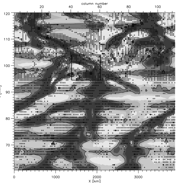
Figure 4: Velocity field distribution in the simulated region at the $\tau_{5}=1$ level, over the course of 60 min. Six shading gradations from dark (downflows) to light (upflows) correspond to vertical velocities (in units of km/s) in the intervals 2, 2–1, 1–0, 0–(-1), (-1)–(-2), $<$(-2). Solid line) zero velocity line. Plus) unusual $V$ profile, square) one-lobe red profiles, diamond) one-lobe blue profiles, triangle) profiles for which their formation conditions were analyzed.

We also plotted the magnetic field strength distribution (Fig. 5). The distribution of areas with fields of different polarities is very nonuniform. Relatively large areas of the same field polarity are met in granulation regions far from strong flux tubes and intense downflows. The largest area with the magnetic field of positive polarity with a strength below 100 mT is outlined by the coordinates $x_{1}=2200$ km, $x_{2}=3500$ km, $t_{1}=85$ min, $t_{2}=100$ min. There are many mixed-polarity fields, one such area can be seen beginning with $t=100$ min. At $t=104$ min and $x=1300$ km two flux tubes came close together and broke down. These flux tubes appear in Fig. 5 as sites with the darkest shading. After the moment $t=104$ min the field structure became heavily complicated throughout the simulation region, there appeared a large number of small areas with opposite polarities and neutral lines.

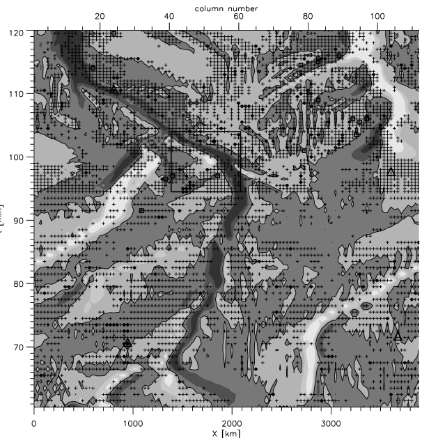
Figure 5: Magnetic field strength distribution at the $\tau_{5}=1$ level. Light shading) positive polarity, dark shading) negative polarity. Solid line) neutral magnetic field lines. Field strength gradations: $>$100, 100–50, 50–0, 0–(-50), (-50)–(-100), $<$(-100) mT. Profile shape designations are the same as in Fig. 4.

Now we examine the position of unusual profiles with respect to the surface structure of magnetic fields. They appear close to neutral lines as well as far from them. One-lobe profiles are met almost without exception along neutral lines, where the field polarity changes. The unusual profiles prefer to cluster in the areas of weak mixed fields below 70 mT, and 12 percent of unusual profiles are met close to strong flux tubes ($B_{z}>70$ mT). It is evident from Table 1 that the probability for an unusual profile to appear near a strong flux tube is greater when the number of lobes in the profile is greater.

We found that large clusters of unusual profiles are always met in the areas with intense downflows, where large granules disintegrate and flux tubes begin to form. An example of such an area can be seen in Fig. 4 and 5 ($x_{1}=3200$ km, $x_{2}=3900$ km, $t_{1}=95$ min, $t_{2}=99$ min). A strong flux tube of positive polarity appeared subsequently in this area.

The occurrence of unusual profiles is different in regions with different magnetic flux – the number of unusual profiles decreases, on the average, with growing mean magnetic field strength $<|B_{z}|>$ in the region (Figs 6a and c). The same tendency was noted earlier in [12]. At the same time the number of unusual profiles tends to decrease when the flux density $<B_{z}>$ differs from zero (Fig. 6b and c) and when the magnetic field of one or other polarity begins to dominate in the region. We can say that this dependence reflects the extent to which fields of different polarities are mixed in the magnetic region. The closer the quantity $<B_{z}>$ to zero, the more pronounced is the alternation of field polarities in the region (cf. Figs 5 and 6).

Figure 6: Temporal changes in the simulation region: a) mean field strength $<|B_{z}|>$ at the $\tau_{5}=1$ level, b) magnetic flux density $<B_{z}>$ at the same level, c) number $N$ of unusual profiles.

So, when we compare the distribution of unusual profiles over the surface with the distributions of velocity, magnetic field strength, and field polarity, it becomes apparent that the presence of mixed-polarity fields and neutral lines is a very important prerequisite to the appearance of unusual profiles. The one-lobe profiles, unlike the multilobe ones, prefer the sites near the neutral line and are often met near the zero line. The fact that the one-lobe profiles are often met at the very edges of granules and lanes rather than in their central parts indicates that they arise under most extreme conditions in passing from one structures to others. The asymmetry of one-lobe and multilobe profiles seems to be of the same origin. To elucidate this problem, we consider in greater detail, with invoking the contribution functions, the formation of these profiles and the effect of the magnetic field and velocity field gradients on their shapes.

Table 3: Distribution of one-lobe profiles over granulation surface.

Type	General number	Granular	Intergranular	Edge
One-lobe profiles	187	82 (43%)	61 (33%)	44 (24%)
One-lobe ”blue“ profiles	109	69 (63%)	23 (21%)	17 (16%)
One-lobe ”red“profiles	78	13 (17%)	38 (49%)	27 (34%)

One-lobe profiles. As would be expected from observation data [26], we found two types of synthetic one-lobe profiles: 58 percent of ”blue“ profiles and 42 percent of ”red“ ones (see an example of ”blue“ profiles in Fig. 2c). We also distinguish granular, intergranular, and marginal one-lobe profiles, in accordance with Fig. 4. Table 3 gives the statistics of the distribution of unusual profiles. The occurrence of one-lobe profiles is greater in the granular regions, and they are predominantly ”blue“ there (84 percent), while in the lanes and at the granule-lane borders ”red“ profiles are met most often (60 percent). Such statistics suggests that the granulation velocity field and velocity gradients have a considerable impact on the formation of one-lobe profiles.

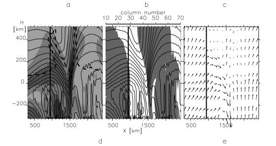
Figure 7: Formation of a granular $V$ profile with blue wing: a) snapshots of magnetic field strength for the simulation region fragment (four shading gradations from dark to light correspond to 70, 70–50, 50–25, 25–0 mT); b) polarity: lighter shading) positive, darker shading) negative; c) velocity field. Thin line) magnetic field lines, thick line) the line of sight along which the profile is calculated, Thick dashed line) level where $\lambda=5000$ K; d) vertical profiles of temperature $T$, velocity $V_{z}$, magnetic field strength $B$ and inclination $\gamma$; e) profiles of depression contribution functions ($CF$) and emerging relative profile intensity ($V/I_{c}$) at various levels in the atmosphere.

Now we consider the formation of ”blue“ profiles with the use of calculated depression contribution functions along the line of sight. Figure 7 illustrates the formation of one of the granular ”blue“ profiles (triangle in Figs 4 and 5, $t=70.5$ min, $x=980$ km, column 28). The upper panel shows the vertical snapshot of a simulation region fragment; the thick solid vertical line is the line of sight along which the selected profile is formed. One can see from the distributions of the field strength (Fig. 7a), field polarity (Fig. 7b), and velocity field (Fig. 7c) that this specific line runs at a distance of 500 km from the center of a magnetic flux tube, it crosses a nearly horizontal magnetic field of negative polarity in deeper layers and positive polarity in upper layers. The field inclination increases in the upper layers due to the magnetic canopy effect. The vertical velocity of ascending flow decreases with increasing height from 2 km/s to zero at the canopy boundary. The vertical profiles of temperature T, velocity $V_{r}$, field strength $B$, and field direction $\gamma$ corresponding to the line of sight are plotted in Fig. 7d. Figure 7e displays the depression contribution function profiles $CF$($\lambda$) at the specified geometric heights $H$ as well as the $V$ profiles obtained by integrating $CF$ along the heights above the given level, i.e., $V/I_{c}(\tau,\lambda)=\int_{\tau}^{0}d\tau_{0}CF(\tau_{0})$. One can see [24] for more information on the calculation of contribution functions $CF(\lambda)$. At the very bottom of the right panel in Fig 7e one can see the one-lobe absorption $V$ profile of the circularly polarized light emerging at the surface.

When the profiles are compared, it is apparent that the level of effective formation of the line $\lambda$ 630.2 nm profile lies in the temperature region about 5000 K. The position of this effective region in the inhomogeneous atmosphere is shown in Fig. 7a by a dashed thick curve on the background of the magnetic field strength distribution. The depression contribution in the profile of emerging polarized radiation are the greatest in every column near this temperature layer. It is significant that temperature rises near flux tubes. This rise is manifested the so-called hot walls which always appear in the upper flux tube layers due to magnetoconvection [4, 6].

Considering the vertical velocity profile ($V_{r}$) in a given column (Fig. 7d) and the velocity pattern in the surrounding space (Fig. 7c), one can notice a flow which is directed towards the flux tube and which fosters the field concentration in the flux tube. The profile we consider here is formed in the region where the velocity gradient changes its sign from negative to positive when going from deeper layers to upper ones. As a result, the blue Doppler shifts of the contribution function profiles are different at different photospheric levels so that the integrated profile is strongly shifted to shorter wavelengths. Thus, a sudden drop of velocity with growing height gave rise to a stronger blue wing in the profile.

As the magnetic field strength decreases with increasing height (Fig. 7d), the magnetic splitting becomes weaker and the distance between the contribution profile lobes decreases, while the change in the magnetic field direction along the line of sight reverses the shape of the contribution function. Due to such intricate combinations of contribution functions, the intensities in the red profile wing compensate one another. The cause of the polarity change along the line of sight is evident from Fig. 7b – this is a kink of magnetic field lines in the region of the ascending convective flow which carries the horizontal magnetic field.

Thus, when all the above-mentioned effects are integrated over all layers, the contributions with opposite signs are compensated in the red wing and are accumulated in the blue wing. The major contribution to profile formation is made in the lower photospheric layers, where the magnetic field has the positive polarity. As a result, the integrated profile has a blue wing with negative amplitude. The polarity change and the negative field strength gradient in the region of profile formation suppress the red wing, while the negative gradient of vertical velocity enhances the blue wing. Our analysis of the formation of a large number of blue one-wing profiles revealed that the negative velocity gradient along the line of sight and the polarity change are typical for them, while the field strength gradient can be negative as well as positive. The field strength gradient along the line of sight can also change its sign. Therefore, the presence of blue profiles in granules suggests that the field polarity changes its sign there, there are significant negative gradients of vertical velocities of upflows, and that various gradients of the weak magnetic field strength can be met. The sign of wing amplitude is indicative of the field polarity in the layer most efficient in the formation of the given profile.

The conditions for the granular red profile formation differ from those for blue profiles in that the upflow velocity gradient is predominantly positive, i.e., the velocity amplitude increases with height (Fig. 8d).

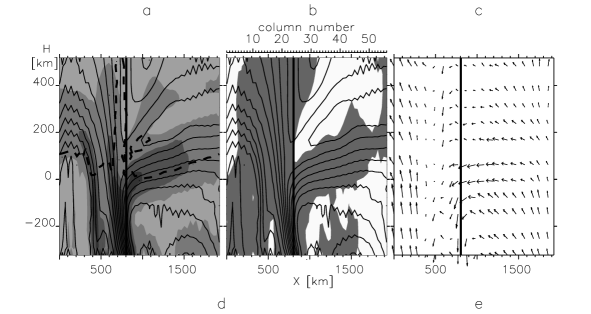
Figure 8: Formation of an integranular $V$ profile with red wing near a strong flux tube (designations are the same as in Fig. 7).

The red profiles are formed in the intergranular lanes with weak magnetic field when downflow velocities in the effective formation region exceed 2 km/s. When the velocities are lower, the probability for a blue wing only to be formed is much higher. If there are strong flux tubes in the lane, the red profiles are formed more often than the blue ones on their periphery. Figure 8 illustrates the formation of an intergranular red profile on the periphery of a strong flux tube ($x=840$ km, $t=110.5$ min, column 24 in Figs 4,5). Steep negative gradients of downflow velocity and field strength can be seen in the effective profile formation region. There also is a small region when the polarity changes its sign. As a result, a quite wide red wing is formed and the blue wing is suppressed.

Red peripheral one-wing profiles as well as blue ones located on the zero line and on the neutral line between granules and lanes are formed in the regions where the velocities are close to zero and their gradients are insignificant so that the gradients of magnetic field strength and direction have a dominant role there.

Our analysis revealed that the one-wing profiles are formed only when the magnetic field polarity changes along the line of sight and when there are the velocity and field strength gradients. So, the appearance of one-wing profiles points unambiguously to the presence of inhomogeneous magnetic fields of different polarities in the photosphere. The shape of these profiles is difficult to use for the diagnostics of physical conditions in magnetic structures, because there are various factors which can affect this shape. First of all, this is a horizontal nonuniformity of the solar surface structure [12]. In this analysis we investigated the profile asymmetry without averaging and found that structure irregularities can occur in inhomogeneous models along the line of sight as well, and they heavily affect the shape of the Stokes profiles. We also found that the shape of one-wing profiles depends on their location on the granular surface of the photosphere. We may state, therefore, that the predominance of blue one-wing profiles in the region observed attests to the domination of almost horizontal weak granular magnetic fields. The predominance of red profiles can testify that there are mixed strong and weak magnetic fields and considerable field strength and velocity gradients in the region.

Multilobe profile. We used the contribution functions to analyze a large number of multilobe profiles and the conditions of their formation. It has been ascertained that in all instances the polarity changed one or more times along the line of sight whatever the profile located may be – near the neutral line, far from it in a granule, or in a lane at a flux tube periphery. Gradients of velocity and field strength also are requisite, with the gradient sign changing very often. The greater the number of lobes in the profile, the more intricate are the gradient profiles.

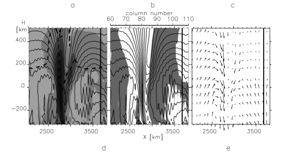
Figure 9: Formation of a typical unusual $V$ profile with three lobes (designations are the same as in Fig.7).

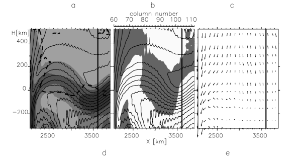
Figure 10: Formation of a typical unusual $V$ profile with four lobes (designations are the same as in Fig. 7).

Figure 9 illustrates the formation of a typical three-lobe profiles which is often met in observations. Column 106 (see Figs 4,5), along which the profile was calculated, is located far from a flux tube in an upflow ($x=3710$ km, $t=71.5$ min). We purposely chose this example so that the velocity gradient might be similar to the gradient considered earlier in the blue one-wing profile in Fig. 7. Nevertheless, the magnetic field gradient is different in these two profiles. Here the field strength decreases with growing height in the profile formation region, and then it increases. It is precisely this gradient sign change that produces a three-lobe profile.

Four-lobe profiles are also often observed. An example of such a profile formed in a stable downflow is seen in Fig. 10 ($x=3640$ km, $t=97.5$ min, column 104 in Figs 4,5). Fragmentation of a large granule and formation of a flux tube begin in this region (Figs 10a–c). These processes are described in detail in [5, 6]. The vertical profiles of atmospheric parameters (Figs 10d, e) indicate that there are two factors which affect the profile shape and give rise to four lobes: ($i$) the strong horizontal magnetic field of about 100 mT which is concentrated in deep photospheric layers and which becomes weaker with increasing height and then remains almost unchanged (this situation is similar to a magnetopause) and ($ii$) the polarity change in the magnetic field carried by an intense plasma flow into deeper layers. The vertical velocity of the downflow has a small gradient and slightly affects the profile shape.

The number of lobes depends on the combination of all asymmetry factors in each specific case. The formation of multilobe profiles is related to more intricate structures of velocity field and magnetic field and to more frequent gradient sign changes. For these profiles it is difficult to find necessary combinations of all three parameters (velocity, field strength, and field inclination) and their gradients. Besides, we do not see any considerable difference between the mechanism of formation of one-lobe and multilobe profiles. They all arise due to polarity changes and changes in the sign of the velocity and field strength gradients.

Thus, the main cause of extreme asymmetry is the growth of magnetic field structurization, which occurs most often not far from intense matter downflows, where flux tubes are being formed, or near already existing strong flux tubes.

5 Discussion and conclusion

We synthesized 9632 Stokes $V$ profiles based on the inhomogeneous model atmospheres obtained in the numerical 2-D solar magnetogranulation simulation [4]. The highest amplitude of the wing in the weakest calculated profile was $|a_{max}|=0.0014$. The number of extremely asymmetric profiles with the number of lobes smaller and greater than two depends on the limit chosen for the amplitude of the minimal lobe. This limit can be taken as one percent for the calculated profiles. To compare our results to observations, we took a limiting amplitude ratio of 25 percent. With this value, the fraction on calculated one-lobe profiles corresponded to observations [26]. The unusual profiles made up 48 and 21 percent of all calculated profiles when the limiting amplitude ratio was 1 and 25 percent, respectively. The results of the observation [29] and of the synthesis with 3-D MHD models [12, 20] suggest that unusual profiles comprise about 35 percent in the profile sample with $|a_{max}|$ greater than 0.0015 or 0.001. The comparison of our results with observations is not sufficiently correct because the number of unusual profiles found in observations was not referred to all observed profiles. There may be some discrepancy caused by differences in the magnetic fluxes and by the use of a two-dimensional approximation in the MHD models. The granulation motions of matter in the 2-D simulated space necessarily differ from actual motions, and this reflects on the magnetic field structure and profile shapes.

The synthesized extremely asymmetric $V$ profiles demonstrated some peculiarities found earlier in the polarimetric observations outside active regions made with a spatial resolution better than one second of arc [11, 26, 29]. Our simulation also revealed that unusual profiles are often grouped near neutral lines and at the periphery of regions with flux tubes, avoiding their central parts. The shapes and shifts of these unusual profiles can be different, the profiles with three and four lobes being of most frequent occurrence.

Our analysis with the use of depression contribution functions confirmed the conclusions made in [12, 17, 20] that the one-lobe Stokes $V$ profiles are formed in the solar photosphere due to the joint action of the gradients of velocity fields and magnetic fields of mixed polarities, with the polarities changing not only on the surface bat along the line of sight as well. The effect of these polarity changes cannot be detected in direct observations, it became evident only in simulations, and it points to a complicated structure of magnetic fields caused by granulation motions.

The new principal results of our investigation of synthesized multilobe profiles are as fallows.

1. Unusual profiles appear predominantly near intense plasma downflows (with velocities of 2 km/s and more) at the borders of granules and lanes.

2. The large groups of unusual profiles observed in the regions with weak fields and intense downflows can be precursors of strong magnetic concentrations in the form of flux in these regions.

3. The one-lobe profiles with well-developed blue wing appear in granules in the main, while in lanes and near the zero line only the profiles with red wing appear.

4. All extremely asymmetric profiles are of the same nature whatever the number of lobes and their shape. The major prerequisite for the formation of unusual profiles is the change of magnetic field polarity along the line of sight (there may be one change or several ones). The gradients of matter velocity, of magnetic field strength and inclination, which are the main cause of usual classical asymmetry, still remain important factors in the formation of unusual profiles, and the number of profile lobes is proportional to the frequency of changes in the sign of the magnetic field strength gradient along the line of sight. Various combinations of all these factors as well as the variability of main atmospheric parameters in the region of profile formation give rise to a great diversity of profile shapes.

Our results give answers to some questions raised in [26] as to the origin of unusual profiles.

Are there most frequently met types of unusual profiles? We found two such types of unusual profiles – with three and four lobes of alternating signs.

What physical processes are responsible for the most frequently met types of unusual profiles? The turbulent and convective motions of plasma and the formation of magnetic concentrations during the fragmentation of big granules are instrumental in producing a complicated structure of magnetic fields with sign-variable gradients of field strength and inclination.

Are one-lobe profiles the extreme case of unusual profiles? They might be reckons as such from the standpoint of profile shape, but as far as the origin of unusual profiles is concerned, the profiles with four and more lobe should be regarded as the extreme case of asymmetry.

Are the unusual profiles a result of mixed polarities on very small scales? It is precisely the polarity changes along the line of sight that are the main cause of extreme profile asymmetry.

Why these unusual profiles have never been observed inside strong kilogauss fields? Strong magnetic flux tubes with field strength of more than 100 mT are almost without exception vertical in the region of profile formation, and no polarity changes occur in this case.

Can profile shapes be used for preliminary diagnostics of observed solar surface areas? The appearance of unusual profiles is indicative of a complicated magnetic field structure in both the horizontal direction and the vertical one, but they say nothing about the field strength. The magnetic fields are often weak and nearly horizontal in the regions of ascending magnetic flux. Sometimes they can be inclined in the magnetic canopy regions not far from flux tubes, and they can be nearly vertical near kilogauss flux tubes.

What is the cause of mixed polarities? What physical processes lead to polarity mixing on very small scales? This is the principal problem, and it needs a more detailed discussion.

There is no doubt that the extreme asymmetry of $V$ profiles with one or several lobes is dictated by the fine magnetic field structure produced by turbulent plasma motions in the regions where the convection penetrates into the photosphere (the magneto-convection processes). Three-dimensional hydromagnetic simulations [35] demonstrated the existence of a complicated surface granulation structure and the crucial importance of intense downdraft in the solar convection. It is these downdraft that control much more extensive ascending convective flow and smaller turbulent motions. The authors of [35] sketched the following broad outlines of solar convection. The ascending warm convective flows have low density and medium entropy. While ascending, they spread in order to conserve mass, since the density is lower in the upper layers. Only a small part of ascending material reaches the surface, where its energy and entropy are carried away by radiation; thus the material density increases, and this heavier material forms a downflow. This descending material forms intensive downdrafts in the lower layers, obeying the law of mass conservation; shifting motions arise at the downflow borders, and they produce eddies and turbulence. To the contrary, in the ascending matter the level of fluctuations is very low because the spreading smooths all disturbances. As a result, we observed laminar upflows and turbulent downflows. When we supplement this picture with a magnetic field, which is frozen in the plasma under the solar plasma conditions, we can easily understand why magnetic field lines have complicated configurations at the borders of granules and lanes.

The relationship between magnetic field and convection was demonstrated in two-dimensional MHD simulations of magneto-convection [1, 4, 5, 6, 34] as well as in three-dimensional ones [36, 38]. Observations [11, 28] and the results of numerical simulations of the Stokes profiles [2, 12, 25] also pointed to a strong interdependence of magnetic fields in quiet regions and local convection processes.

In this study, which is based on the results of the Stokes profile synthesis and the 2D-MHD simulations of nonstationary magneto-convection, we demonstrated that the main cause of the formation of unusually shaped profiles is the complicated structure of the magnetic field with its polarity changing along the line of sight and the complicated gradients of velocity and field strength at granule and lane borders. Such conditions favorable for the formation of unusual profiles arise due to the local turbulence produced in the surface magneto-convection by shifting motions at the borders of powerful downflows.

Acknowledgements. The author wishes to thank S. Solanki, S. Ploner, M. Schüssler, and E. Khomenko for their useful comments and discussions of the results. This study is a part of an international program, it was partially financed by INTAS (Grant No.00084).

References

- [1] I. N. Atroschenko and V. A. Sheminova, Kinematika i Fizika Nebes. Tel [Kinematics and Physics of celestial Bodies], vol. 12, no. 4, pp. 32–45, 1996.
- [2] F. Cattaneo, Astrophys. J., vol. 515, no. 1, pp. L39–L42, 1999.
- [3] C. Frutiger and S. K. Solanki, Astron. and Astrophys., vol. 336, no. 2, pp. L65–L68, 1998.
- [4] A. S. Gadun, Kinematika i Fizika Nebes. Tel [Kinematics and Physics of Celestial Bodies], vol. 16, no. 2, pp. 99–120, 2000.
- [5] A. S. Gadun, V. A. Sheminova, and S. K. Solanki, Kinematika i Fizika Nebes. Tel [Kinematics and Physics of Celestial Bodies], vol. 15, no. 5, pp. 387–397, 1999.
- [6] A. S. Gadun, S. K. Solanki, V. A. Sheminova, and S. R. O. Ploner, Solar Phys., vol. 203, no. 1, pp. 1–7, 2001.
- [7] U. Grossmann-Doerth, C. U. Keller, and M. Schüssler, Astron. and Astrophys., vol. 315, no. 3, pp. 610–617, 1996.
- [8] U. Grossmann-Doerth, M. Schüssler, M. Sigwardth, and O. Steiner, Astron. and Astrophys., vol. 357, no. 1, pp. 351–358, 2000.
- [9] U. Grossmann-Doerth, N. Schüssler, and O. Steiner, Astron. and Astrophys., vol. 337, no. 3, pp. 928–939, 1998.
- [10] C. U. Keller, F.-L. Deubner, U. Egger, et al., Astron. and Astrophys., vol. 286, no. 2, pp. 626–634, 1994.
- [11] E. V. Khomenko, M. Collados, S. K. Solanki, et al., Astron. and Astrophys., vol. 408, no. 2, pp. 1115–1135, 2003.
- [12] E. V. Khomenko, S. Shelyag, S. K. Solanki, et al., in: Multi-Wavelength Investigations of Solar Activity. IAU Symp. No. 223, A. V. Stepanov, E. E. Benevolenskaya, and A. G. Kosovichev (Editors), pp. 635–636, Cambridge Univ. Press, Cambridge, 2004.
- [13] O. Kjeldseth Moe, in: Structure and Development of Solar Active Regions. IAU Symp. No. 35, K. O. Kiepenheuer (Editor), pp. 202–210, Reidel, Dordrecht, 1968.
- [14] B. W. Lites, K. D. Leka, A. Skumanich, et al., Astrophys. J., vol. 460, no. 1, pp. 1019–1026, 1996.
- [15] V. Mártinez Pillet, B. W. Lites, and A. Skumanich, Astrophys. J., vol. 474, no. 2, pp. 810–842, 1997.
- [16] S. R. O. Ploner, M. Schüssler, S. K., Solanki, and A. S. Gadun, in: Theory, Observation, and Instrumentation, pp. 363–370, M. Sigwarth (Editor), ASP Conf. Ser., vol. 236, 2001.
- [17] S. R. O. Ploner, M. Schüssler, S. K. Solanki, et al., in: Theory, Observation, and Instrumentation, pp. 371–378, M. Sigwarth (Editor), ASP Conf. Ser., vol. 236, 2001.
- [18] I. Rüedi, S. K. Solanki, W. Livingston, and J. O. Stenflo, Astron. and Astrophys., vol. 263, no. 1/2, pp. 323–338, 1992.
- [19] I. Rüedi, S. K. Solanki, and D. Rabin, Astron. and Astrophys., vol. 261, no. 2, pp. L21–L24, 1992.
- [20] J. Sánchez Almeida, T. Emmonet, and F. Cattaneo, Astrophys. J., vol. 585, no. 1, pp. 536–552, 2003.
- [21] J. Sánchez Almeida, E. Landi degl’Innocenti, V. Martinez Pillet, and B. W. Lites, Astrophys. J., vol. 466, no. 1, pp. 537–548, 1996.
- [22] J. Sánchez Almeida, and B. W. Lites, Astrophys. J., vol. 532, no. 2, pp. 1215–1229, 2000.
- [23] M. Schüssler, in: Solar Polarization. ASP Conf. Ser., vol. 307, pp. 601–613, J. Trujillo Bueno and J. Sanchez Almeida (Editors). 2003.
- [24] V. A. Sheminova, Kinematika i Fizika Nebes. Tel [Kinematics and Physics of Celestial Bodies], vol. 8, no. 3, pp. 44–62, 1992.
- [25] V. A. Sheminova, Kinematika i Fizika Nebes. Tel [Kinematics and Physics of Celestial Bodies], vol. 15, no. 5, pp. 398–411, 1999.
- [26] M. Sigwarth, Astrophys. J., vol. 563, no. 1, pp. 1031–1044, 2001.
- [27] M. Sigwarth, K. S. Balasubramaniam, M. Knölker, and W. Schmidt. Astron. and Astrophys., vol. 349, no. 3, pp. 941–955, 1999.
- [28] H. Socas-Navarro, V. Martínez Pillet, and B. W. Lites, Astrophys. J., vol. 611, no. 2, pp. 1139–1148, 2004.
- [29] H. Socas-Navarro and J. Sánchez Almeida, Astrophys. J., vol. 565, no. 2, pp. 1223–1334, 2002.
- [30] S. K. Solanki, Space Sci. Rev., vol. 31, pp. 1–188, 1993.
- [31] S. K. Solanki and C. A. Montavon, Astron. and Astrophys., vol. 275, no. 1, pp. 283–292, 1993.
- [32] H. C. Spuit, A. M. Title, and A. A. van Ballegooijen, Solar Phys., vol. 110, no. 1, pp. 115–128, 1987.
- [33] O. Stiener, Solar Phys., vol. 196, no. 2, pp. 245–268, 2000.
- [34] O. Steiner, U. Grossmann-Doerth, M. Knölker, and M. Schüssler, Astrophys. J., vol. 495, no. 1, pp. 468–484, 1998.
- [35] R. F. Stein and Å. Nordlund, Astrophys. J., vol. 499, no. 2, pp. 914–933, 1998.
- [36] R. F. Stein and Å. Nordlund, in: SOLMAG 2002. Proc. of the Magnetic Coupling of the Solar Atmosphere Euroconference and IAU Colloquium 188, 11–15 June 2002, Santorini, Greece, H. Sawaya-Lacoste (Editor), pp. 83–89, ESA Publ. Division, Noordwijk, 2002. (ESA SP-505).
- [37] S. I. Vainshtein, Ya. B. Zel’dovich, and A. A. Ruzmaikin, Turbulent Dynamo in Astrophysics [in Russian], Nauka, Moscow, 1980.
- [38] A. Vögler, S. Shelyag, M. Schüssler, et al., Astron. and Astrophys., vol. 429, no. 1, pp. 335–351, 2005.