Magnetic field induced semimetal-to-canted-antiferromagnet transition
on the honeycomb lattice

Abstract

It is shown that the semimetallic state of the two-dimensional honeycomb lattice with a point-like Fermi surface is unstable towards a canted antiferromagnetic insulator upon application of an in-plane magnetic field. This instability is already present at the mean-field level; the magnetic field shifts the up- and the down-spin cones in opposite directions thereby generating a finite density of states at the Fermi surface and a perfect nesting between the up- and the down-spin Fermi sheets. This perfect nesting triggers a canted antiferromagnetic insulating state. Our conclusions, based on mean-field arguments, are confirmed by auxiliary field projective quantum Monte Carlo methods on lattices up to $12\times 12$ unit cells.

I Introduction

Graphene, or the physics of electrons on the honeycomb lattice, has recently received tremendous attention due to its semimetallic nature with low-energy quasiparticles behaving as massless Dirac spinors; a recent review can be found in Ref. Castro Neto et al. (2009). A crucial point is the stability of this semimetallic phase to particle-hole pairing. In particular, research activities have been devoted to the investigation of magnetic field induced transitions as a function of magnetic fields Aleiner et al. (2007); Kempa et al. (2003); Kharzeev et al. (2006) and electronic correlations. Sorella and Tosatti (1992); Paiva et al. (2005); Herbut (2006); Raghu et al. (2008) The vanishing density of states at the Fermi energy protects the semimetallic state against weak correlations. Notably, a finite critical value of the repulsive Hubbard interaction $U/t$ is required to destabilize the semimetallic state in favor of an antiferromagnetic Mott insulator. Sorella and Tosatti (1992); Paiva et al. (2005); Herbut (2006)

In this paper, we will argue that the semimetallic state is unstable against the application of an in-plane magnetic field. The mechanism behind this instability can be understood already at the mean-field level. Milat (2004); Beach (2006); Peres (2004) The magnetic field generates a finite Fermi surface density of states. A Stoner instability for arbitrarily small values of the Coulomb repulsion arises from the perfect nesting of the spin split Fermi sheets. This triggers antiferromagnetic order with staggered magnetization perpendicular to the applied magnetic field and the opening of a charge gap. That the application of an in-plane magnetic field in the continuum limit facilitates a spontaneous symmetry breaking has already been pointed out in Ref. Kharzeev et al. (2006). The purpose of this paper is to show that those mean-field arguments indeed capture the correct physics, since exact quantum Monte Carlo (QMC) simulations on the honeycomb lattice compare favorably with those mean-field results.

The outline of the paper is as follows. In Sec. II the model Hamiltonian is introduced and its mean-field solution is discussed. The projective QMC method for ground state properties and numerical results are presented in Sec. III. The last section, Sec. IV, contains the summary and the conclusions, also with respect to the experimental relevance of our findings.

II Model Hamiltonian and mean-field treatment

Our starting point is the Hubbard model on the honeycomb lattice shown in Fig. 1.

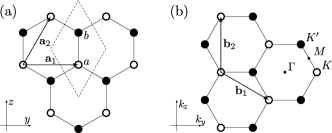
Figure 1: (a) Real and (b) reciprocal space lattice vectors of the honeycomb lattice, ${\mathbf{a}_{1}=a_{0}\;(0,1,0)}$, ${\mathbf{a}_{2}=a_{0}\;(0,1/2,\sqrt{3}/2)}$ and ${\mathbf{b}_{1}=2\pi/a_{0}\;(0,1,-1/\sqrt{3})}$, ${\mathbf{b}_{2}=2\pi/a_{0}\;(0,0,2/\sqrt{3})}$, with $a_{0}$ being the lattice constant. The unit cell with the orbitals $a$ and $b$ is indicated by the dashed diamond shape. Filled (empty) circles denote sites on the same sublattice.

$$H = H_{0}+H_{U}+H_{B},$$

$$H_{0} = -t\sum_{{\bf i},{\bf r},\sigma}\Big{(}\hat{a}^{\dagger}_{{\bf i},\sigma}\hat{b}_{{\bf i}+{\bf r},\sigma}+\hat{b}^{\dagger}_{{\bf i}+{\bf r},\sigma}\hat{a}_{{\bf i},\sigma}\Big{)},$$

$$H_{U} = U\sum_{l=a,b}\sum_{{\bf i}}\left(\hat{n}_{{\mathbf{i},l},\uparrow}-1/2\right)\left(\hat{n}_{{\mathbf{i},l},\downarrow}-1/2\right),$$

$$H_{B} = \frac{g}{2}\mu_{\mathrm{B}}B\sum_{l=a,b}\sum_{{\bf i},\sigma}p_{\sigma}\hat{n}_{{\mathbf{i},l},\sigma}\;.$$ (1)

The electron operator $\hat{a}^{\dagger}_{{\bf i},\sigma}$ ($\hat{b}^{\dagger}_{{\bf i},\sigma}$) creates an electron on the orbital $a$ ($b$) in the unit cell ${\bf i}$ and the associated electron-density operator is ${\hat{n}^{l}_{{\bf i},\sigma}=\hat{a}^{\dagger}_{{\bf i},\sigma}\hat{a}_{{\bf i},\sigma}}$ (${\hat{b}^{\dagger}_{{\bf i},\sigma}\hat{b}_{{\bf i},\sigma}}$), for $l=a$ ($b$). Owing to the bipartite nature of the lattice, hopping with matrix element $t$ occurs only between the $a$ and the $b$ orbitals of unit cells related by lattice vector ${\bf r}$ in the three directions $\left\{{\bf 0},{\bf a}_{1}-\bf{a}_{2},-{\bf a}_{2}\right\}$. The on-site electron-electron repulsion is denoted by $U>0$ and $p_{\sigma}=\pm 1$ for $\sigma=\uparrow,\downarrow$. In the present case of half filling the chemical potential vanishes. In the following, we set $(g/2)\mu_{\mathrm{B}}\equiv 1$. We have included only a Zeeman coupling to the magnetic field. Hence, for comparison with experiments, we can only consider setups with magnetic field orientations parallel to the lattice plane since only in this case we can neglect the orbital coupling.

The Hamiltonian $H_{0}$ gives rise to two bands,

$$\lambda_{n}({\bf k})=p_{n}\left|t\sum_{\bf r}e^{-i{\bf k}\cdot{\bf r}}\right|,$$ (2)

with $p_{n}=\pm 1$ for $n=1,2$, respectively. At half-band filling the Fermi surface consists of two points, $K,K^{\prime}$ in Fig. 2, with density of states

$$\rho(\omega)=\frac{1}{N}\sum_{\bf k}\delta\left(\omega-\lambda_{1}[{\bf k}]\right).$$ (3)

Here, $N$ corresponds to the lattice size and linearization of the dispersion relation around $K$ and $K^{\prime}$ yields: $\rho(\omega)\propto\omega/t^{2}$ for $\omega\ll t$.

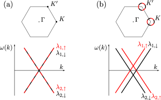
Figure 2: Visualization of the nesting of spin-up and spin-down Fermi surfaces. In case of (a) $B=0$ the spin bands collapse onto each other, whereas for (b) $B>0$ the bands are shifted by virtue of the magnetic field leading to the nesting relation ${\lambda_{1,\uparrow}(\mathbf{k})=-\lambda_{2,\downarrow}(\mathbf{k})}$.

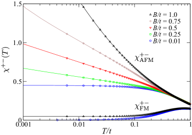
Figure 3: (Anti-)ferromagnetic susceptibilities ${\chi^{+-}_{\mathrm{(A)FM}}(\mathbf{Q})}$ for the magnetic fields $B/t=0.01,...,1.0$.

Prior to examining the mean-field Hamiltonian we demonstrate the instability of the non-interacting system when turning on the magnetic field. Consider the transverse magnetic susceptibility tensor:

$$\begin{pmatrix}\chi^{+-}_{aa}(\mathbf{q})&\chi^{+-}_{ab}(\mathbf{q})\\ \chi^{+-}_{ba}(\mathbf{q})&\chi^{+-}_{bb}(\mathbf{q})\end{pmatrix}=\begin{pmatrix}\chi^{+-}_{d}(\mathbf{q})&\chi^{+-}_{o}(\mathbf{q})\\ \chi^{+-}_{o}(\mathbf{q})&\chi^{+-}_{d}(\mathbf{q})\end{pmatrix}\;.$$ (4)

Here $\chi^{+-}_{l,l^{\prime}}(\mathbf{q})=\int_{0}^{\beta}d\tau\langle S^{+}_{l}(\mathbf{q},\tau)S^{-}_{l^{\prime}}(-\mathbf{q},0)\rangle$ and the indices $l,l^{\prime}=a,b$ label the sublattices. $\beta$ corresponds to the inverse temperature and the spin raising and lowering operators read $S^{+}_{a}(\mathbf{q})=\frac{1}{\sqrt{N}}\sum_{{\bf i}}e^{-i{\bf q}\cdot{\bf i}}\hat{a}^{\dagger}_{{\bf i},\uparrow}\hat{a}_{{\bf i},\downarrow}$ and $S^{-}_{a}(\mathbf{q})=\frac{1}{\sqrt{N}}\sum_{{\bf i}}e^{-i{\bf q}\cdot{\bf i}}\hat{a}^{\dagger}_{{\bf i},\downarrow}\hat{a}_{{\bf i},\uparrow}$, respectively. Similar definitions hold for the $b$ sublattice. The eigenvectors of the magnetic susceptibility tensor are given by

$$\begin{gathered}\chi^{+-}_{\mathrm{FM}}(\mathbf{q})=\chi^{+-}_{d}(\mathbf{q})+\chi^{+-}_{o}(\mathbf{q}),\\ \chi^{+-}_{\mathrm{AFM}}(\mathbf{q})=\chi^{+-}_{d}(\mathbf{q})-\chi^{+-}_{o}(\mathbf{q}),\end{gathered}$$ (5)

and correspond, respectively, to the ferromagnetic and the antiferromagnetic alignments of spins within the unit cell. Nesting occurs at $\mathbf{q}=\mathbf{Q}=(0,0)$ and leads to a logarithmic divergence of the antiferromagnetic mode at finite values of the magnetic field (Fig. 3).

$$\chi^{+-}_{\mathrm{FM}}\left({\mathbf{Q}}\right) = \frac{1}{4NB}\sum_{\mathbf{k}}\sum_{n=1}^{2}\Big{(}f\big{(}\lambda_{n,\downarrow}(\mathbf{k})\big{)}-f\big{(}\lambda_{n,\uparrow}(\mathbf{k})\big{)}\Big{)}$$ (6a)

$$= \frac{1}{4B}\int d\omega\Big{[}\rho(\omega-B)-\rho(\omega+B)\Big{]}$$

$$\times\;\Big{(}f(-\omega)-f(\omega)\Big{)}\;,$$

and

$$\chi^{+-}_{\mathrm{AFM}}\left({\mathbf{Q}}\right) = \frac{1}{2N}\sum_{\mathbf{k}}\sum_{\begin{subarray}{c}n,m=1\\ n\neq m\end{subarray}}^{2}\frac{f\big{(}\lambda_{n,\downarrow}(\mathbf{k})\big{)}-f\big{(}\lambda_{m,\uparrow}(\mathbf{k})\big{)}}{\lambda_{m,\uparrow}(\mathbf{k})-\lambda_{n,\downarrow}(\mathbf{k})}$$ (6b)

$$= \frac{1}{4}\int d\omega\Big{[}\rho(\omega-B)+\rho(\omega+B)\Big{]}$$

$$\times\;\frac{f(-\omega)-f(\omega)}{\omega}\;.$$

In the above,

$$\lambda_{n,\sigma}({\bf k})=\lambda_{n}({\bf k})+p_{\sigma}B$$ (7)

are single-particle states of $H_{0}+H_{B}$ and $f(\omega)=\frac{1}{1+e^{\beta\omega}}$ is the Fermi function. In the low-temperature limit, one can approximate the integral of Eq. (6b) to obtain

$$\chi^{+-}_{\mathrm{AFM}}({\bf Q})\propto\begin{cases}\rho(B)\ln\Big{(}\frac{W}{2k_{\mathrm{B}}T}\Big{)},&|B|>0\\ \text{constant},&B=0\;,\end{cases}$$ (8)

where $W$ corresponds to the bandwidth. Clearly, the divergence of the transverse susceptibility in the antiferromagnetic channel stems from the nesting property, ${\lambda_{1,\uparrow}(\mathbf{k})=-\lambda_{2,\downarrow}(\mathbf{k})}$. At zero magnetic field, this instability is cut off by the vanishing density of sates $\rho(\omega)\propto\omega/t^{2}$. At $B>0$ the low-energy density of states is finite thereby revealing the nesting instability.

Given the above instability, the mean-field Hamiltonian is derived by assuming the magnetization ${\bf m}$ to be alternating on the sublattices: $\mathbf{m}_{l}=\begin{pmatrix}0,&m_{\perp}(-1)^{l},&m_{\parallel}\end{pmatrix}$ with the index $l=0,1$ referring to the orbitals in the unit cell. That is, the magnetization ${\bf m}$ has a constant component $m_{\parallel}$ parallel to the field axis and a staggered component $m_{\perp}$ in the plane perpendicular to the field.

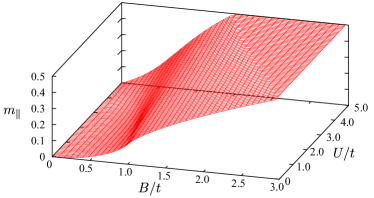
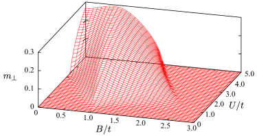
Figure 4: (a) Parallel magnetization $m_{\parallel}$ and (b) staggered magnetization $m_{\perp}$ vs $U$ and $B$, obtained by numerically solving the gap equations, (11).

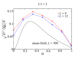
(a)

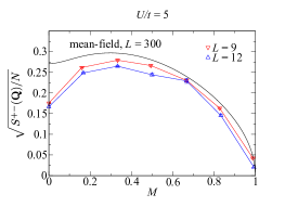
(b)

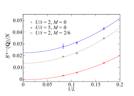
(c)

(d) Staggered magnetization $\sqrt{S^{+-}(\mathbf{Q})/N}$ (a) below and (b) above the critical interaction strength. (c) Finite-size extrapolation of $S^{+-}(\mathbf{Q})/N$. In the semimetallic phase, $U/t=2$, the data are consitent with the onset of transverse staggered order at finite magnetization $M$. For comparison, we have plotted the $U/t=5$ data in the absence of a magnetic field. This value of the Hubbard interaction places us in the antiferromagnetic Mott insulating state.

To decouple the interaction part of the Hamiltonian we rewrite it as ${H_{U}=-\frac{2}{3}U\sum_{l=a,b}\sum_{{\bf i}}\hat{{\bf S}}_{{\bf i},l}^{2}}$, with $\hat{{\bf S}}_{{\bf i},l}$ being the spin-1/2 operator, and the fluctuation term of ${\hat{{\bf S}}_{{\bf i},l}^{2}=[{\bf m}_{l}+(\hat{\bf S}_{{\bf i},l}-{\bf m}_{l})]^{2}}$ is omitted. With this ansatz, the mean-field Hamiltonian mixes the up- and the down-spin sectors thereby yielding four quasiparticle bands:

$$H_{\mathrm{MF}} = \sum_{\mathbf{k}}{\sum_{n,m=1}^{2}{E_{n,m}(\mathbf{k})\;\hat{\gamma}_{n,m,\mathbf{k}}^{\dagger}\hat{\gamma}_{n,m,\mathbf{k}}}}$$ (9)

$$+\;\frac{4}{3}\,UN\big{(}m_{\parallel}^{2}+m_{\perp}^{2}\big{)},$$

with

$$E_{n,m}(\mathbf{k})=p_{m}\sqrt{\big{(}\lambda_{n}({\bf k})+B_{\mathrm{eff}}\big{)}^{2}+\Delta_{\perp}^{2}}\;.$$ (10)

Here, ${p_{m}=\pm 1}$, ${B_{\mathrm{eff}}=B-\Delta_{\parallel}}$, ${\Delta_{\parallel}=\frac{2}{3}Um_{\parallel}}$, and ${\Delta_{\perp}=\frac{2}{3}Um_{\perp}}$. Minimizing the free energy with respect to $m_{\parallel}$ and $m_{\perp}$ yields the gap equations

$$1= \frac{U}{6N}\sum_{\mathbf{k}}\sum_{n=1}^{2}\frac{1}{\sqrt{\left(\lambda_{n}(\mathbf{k})+B_{\mathrm{eff}}\right)^{2}+\Delta_{\perp}^{2}}}$$

$$= \frac{U}{6}\int d\omega\frac{\rho(\omega+B_{\mathrm{eff}})+\rho(\omega-B_{\mathrm{eff}})}{\sqrt{\omega^{2}+\Delta_{\perp}^{2}}},$$ (11a)

$$m_{\parallel}= \frac{1}{4N}\sum_{\mathbf{k}}\sum_{n=1}^{2}\frac{-\left(\lambda_{n}(\mathbf{k})+B_{\mathrm{eff}}\right)}{\sqrt{\left(\lambda_{n}(\mathbf{k})+B_{\mathrm{eff}}\right)^{2}+\Delta_{\perp}^{2}}}$$

$$= \frac{1}{4}\int d\omega\frac{\Big{(}\rho(\omega+B_{\mathrm{eff}})-\rho(\omega-B_{\mathrm{eff}})\Big{)}\omega}{\sqrt{\omega^{2}+\Delta_{\perp}^{2}}}.$$ (11b)

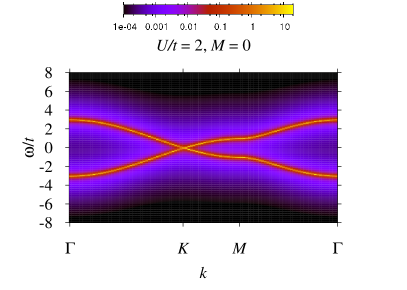
(e)

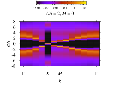
(f)

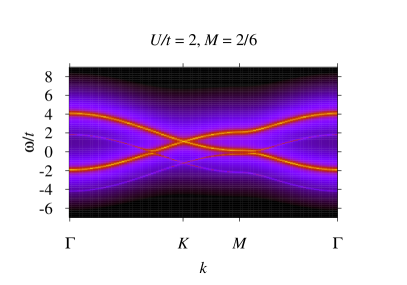
(g)

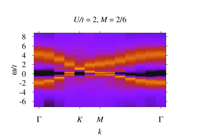
(h)

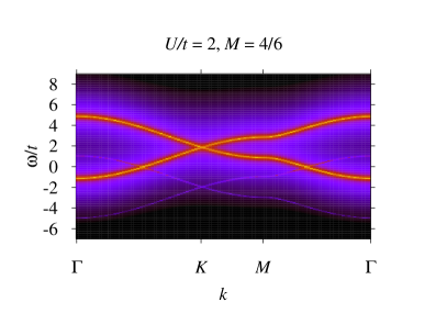
(i)

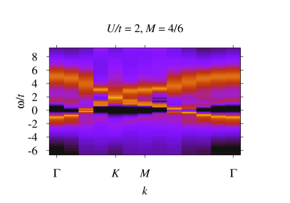
(j)

(k) Single-particle spectral function ${A^{\uparrow}(\mathbf{k},\omega)}$ at $U/t=2$, based on the mean-field (left) and the QMC (right) calculations, respectively. The magnetization $M$ takes the values of $0$, $2/6$, and $4/6$ (from top to bottom). For the intermediate value of the magnetization, one can clearly see the opening of a quasiparticle gap and the avoided level crossing as $m_{\perp}$ acquires a finite value. In general, the magnitude of the gap tracks $m_{\perp}$ [Fig. II(a)]. The QMC spectral functions were obtained via analytical continuation of the Green’s functions with the stochastic maximum entropy method. For the QMC calculations, the lattice size was set to $12\times 12$ unit cells. The legends at the top indicate the false color values.

Our mean-field results are plotted in Figs. 4, II(a), II(c), and II(e). At zero magnetic field, we observed as a function of $U/t$ the expected transition from the semimetallic state (${\bf m}=0$) at ${U/t<U_{c}/t\approx 3.3}$ to the antiferromagnetic Slater insulator characterized by ${|m_{\perp}|>0}$. The semimetallic state at $B=0$ is characterized by the spin degenerate dispersion relation, $\lambda_{n,\sigma}({\bf k})$, as shown in Fig. II(a). Ramping up the magnetic field lifts this degeneracy thereby producing nested Fermi sheets of opposite spin indices. Hence, and irrespective of the magnitude of $U<U_{c}$, energy can be gained by ordering the spins in a canted antiferromagnet. The energy gain corresponds to the gap which in the weak coupling limit, and by virtue of Eq. (11a), takes the form

$$\Delta_{\perp}\cong We^{-3/2U\rho(B_{\mathrm{eff}})}.$$ (12)

The dispersion relation of this canted antiferromagnetic state is plotted in Fig. II(c). To compare at best with the QMC simulations we consider the quantity

$$A^{\uparrow}({\boldsymbol{k}},\omega)=-\frac{1}{\pi}{\rm Im}\left[G^{\uparrow}_{aa}({\boldsymbol{k}},\omega)+G^{\uparrow}_{bb}({\boldsymbol{k}},\omega)\right]$$ (13)

with a finite broadening. As apparent, the features with dominant weight follow the dispersion relation $\lambda_{1,\uparrow}({\bf k})$ and $\lambda_{2,\uparrow}({\bf k})$ and a gap at the Fermi level is apparent. Due to the transverse staggered moment, mixing between the up and the down dispersion relations occurs thereby generating shadow features following the dispersion relations of $\lambda_{1,\downarrow}({\bf k})$ and $\lambda_{2,\downarrow}({\bf k})$. The intensity of the shadow features tracks $m_{\perp}$. As apparent from Fig. 4 the growth of $m_{\perp}$ as a function of the magnetic field is countered by the polarization of the spins along the magnetic field. It is interesting to note that irrespective of $U/t$ the maximal value of $m_{\perp}$ and hence of the magnetic field induced gap is at $B=1$ corresponding to an energy scale matching the position of the Van Hove singularity in the non-interacting density of states. At this point a maximal amount of energy can be gained by the opening of the gap.

Particle-hole symmetry can be exploited to map the repulsive Hubbard model onto an attractive Hubbard model where ${U<0}$ tunes the transition from a semimetal to an $s$-wave superconductor. Scalettar et al. (1989) The external magnetic field driving the semimetal to a canted antiferromagnet in the positive-$U$ model translates to doping the negative-$U$ model which triggers a transition to a uniform superfluid phase with $s$-wave pairing, accordingly. Zhao (2006) In the case of $B=0$ the self-consistent equation for the staggered magnetization, Eq. (11a), is identical to the BCS gap equation for the attractive-$U$ case at half filling.

III Projector quantum Monte-Carlo method

To confirm our mean-field results, we have carried out projector auxiliary field QMC calculations. This PQMC algorithm is based on the equation

$$\frac{\langle\Psi_{0}|A|\Psi_{0}\rangle}{\langle\Psi_{0}|\Psi_{0}\rangle}=\underset{\theta\rightarrow\infty}{lim}\frac{\langle\Psi_{T}|e^{-\theta H}Ae^{-\theta H}|\Psi_{T}\rangle}{\langle\Psi_{T}|e^{-2\theta H}|\Psi_{T}\rangle}\;.$$ (14)

The trial wave function $|\psi_{T}\rangle$ has to be non-orthogonal to the ground state wave function, $\langle\psi_{T}|\psi_{0}\rangle\neq 0$ and the ground state is assumed to be non-degenerate. For the details of the formulation of this approach, we refer the reader to Ref. Assaad and Evertz (2008). In this canonical approach, we fix the magnetization

$$M=\frac{N_{\uparrow}-N_{\downarrow}}{N_{\uparrow}+N_{\downarrow}}$$ (15)

rather than the magnetic field (just as a magnetic field would induce a magnetization). The magnetization $M$ in the QMC algorithm corresponds to the mean-field magnetization $m_{\parallel}$. $N_{\sigma}$ corresponds to the total number of electrons in the spin sector $\sigma$. Furthermore, due to the particle-hole symmetry, which locks in the signs of the fermionic determinants in both spin sectors one can avoid the so-called negative sign problem irrespective of the choice of the magnetization. In practice, for each finite system, we choose a value of the projection parameter $\theta$ large enough so as to guarantee convergence within statistical uncertainty.

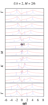
(l)

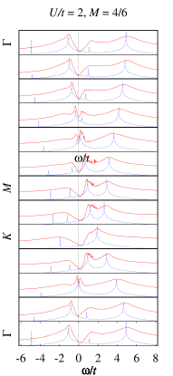
(m)

(n) The plot directly compares the QMC (red) spectral intensity profiles $A^{\uparrow}(\mathbf{k},\omega)$ against the mean-field solution (blue, dotted). Same parameters as in Fig. II.

To detect transverse staggered magnetic order under an applied magnetic field, we have computed the spin-spin correlation functions

$$S^{+-}(\mathbf{q})=\frac{1}{N}\sum_{\mathbf{i},\mathbf{j}}e^{-\i\mathbf{q}(\mathbf{i}-\mathbf{j})}\langle S^{+}_{a}(\mathbf{i})S^{-}_{a}(\mathbf{j})-S^{+}_{a}(\mathbf{i})S^{-}_{b}(\mathbf{j})\rangle\;.$$ (16)

If long-range staggered magnetic order perpendicular to the applied field direction is present, then

$$\sqrt{\lim_{N\rightarrow\infty}\frac{S^{+-}(\mathbf{Q})}{N}}=m^{\mathrm{QMC}}_{\perp}$$ (17)

acquires a finite value. We have computed this quantity on $6\times 6$, $9\times 9$, and $12\times 12$ lattices, and our results are plotted in Fig. II both for $U<U_{c}$ and $U>U_{c}$. At $U/t=2<U_{c}/t$ and zero magnetization, $M=0$, our results are consistent with $m^{\mathrm{QMC}}_{\perp}=0$ whereas, at $M=2/6$, $m^{\mathrm{QMC}}_{\perp}$ takes a finite value. Although we cannot reproduce the essential singularity of the mean-field calculation at $U<U_{c}$, the overall form of the transverse staggered magnetization compares favorably with the mean-field results [see Figs. II(a) and  II(b)] both at $U<U_{c}$ and $U>U_{c}$.

Within the PQMC, the zero-temperature single-particle Green’s function along the imaginary time axis can be computed efficiently with methods introduced in Ref. Feldbacher and Assaad (2001). From this quantity, we can obtain the spectral function of Eq. (13) with the use of a stochastic formulation of the maximum entropy method. Beach (2004); Sandvik (1998) The so obtained results for $A^{\uparrow}({\bf k},\omega)$ are plotted in Figs. II(b),  II(d), and  II(f). As apparent the features in the QMC calculation which are associated with substantial spectral weight are well reproduced by the mean-field calculation. The particle-hole transformation, ${\hat{a}}^{\dagger}_{{\bf i},\sigma}\rightarrow{\hat{a}}_{{\bf i},-\sigma}$ and ${\hat{b}}^{\dagger}_{{\bf i},\sigma}\rightarrow-{\hat{b}}_{{\bf i},-\sigma}$, leads to the relation

$$A^{\uparrow}({\bf k},\omega)=A^{\downarrow}({\bf k},-\omega).$$ (18)

At finite magnetic fields or equivalently at finite magnetizations, the staggered transverse order leads to a gapless Goldstone mode of which the quasiparticle can spin-flip scatter. As a consequence, and as already observed in the mean-field calculation, the features of the down spectral function should be visible in $A^{\uparrow}({\bf k},\omega)$. Upon inspection of Fig. III one will observe that for each dominant low-energy peak at $\omega({\bf k})$ in $A^{\uparrow}({\bf k},\omega)$ a shadow feature at $-\omega({\bf k})$ is present.

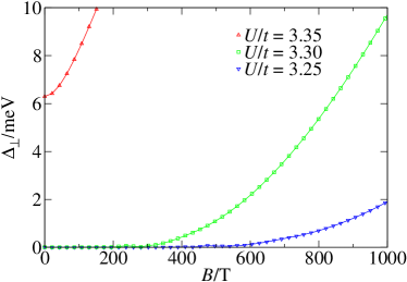
Figure 5: Charge gap $\Delta_{\perp}$ as a function of the applied magnetic field for $t=2.5$eV, obtained by numerically solving the gap equations, (11).

IV Summary and Conclusions

In conclusion, we have carried out mean-field calculations and projective quantum Monte Carlo simulations for the Hubbard model on the honeycomb lattice in a magnetic field oriented parallel to the lattice plane. With this setup, only the Zeeman spin coupling is present. Our results show the inherent instability of the semimetallic state to a canted antiferromagnet upon application of the magnetic field. Ramping up the magnetic field generates nested up and down Fermi surfaces with finite density of states. As a consequence, the onset of canted antiferromagnetic order opens a charge gap and provides an energy gain irrespective of the magnitude of the Hubbard repulsion.

Experimentally, such a transition could be observed by magneto resistance measurements. The transition to the canted antiferromagnet breaks a U($1$) symmetry and hence occurs at finite temperatures $T_{\mathrm{KT}}$ in terms of a Kosterlitz-Thouless transition. Below $T_{\mathrm{KT}}$ the power-law decay of the transverse spin-spin correlation function should suffice to produce a visible pseudo-gap in the charge sector and hence an increase in the resistivity as a function of decreasing temperature. The primary issue to observe the transition is the magnitude of the required magnetic field so as to obtain a visible gap. With $t\approx 2.5-3.0$eV and $U\approx 10-16$eV, ParrBaer (2004) one can readily see that very large magnetic fields will be required to obtain charge gaps in the meV region. In particular, in Fig. 5 we plot the charge gap in meV as a function of $B$ in tesla for values of the Coulomb repulsion close to $U_{c}$. The g factor has been set to the (approximate) free-electron value, $g=2$. As apparent, depending on $U$, values on the order of $B\propto 10^{2}-10^{3}$T are required to obtain an acceptable gap. Clearly those numbers imply that the only feasible manner to observe this effect would be to grow graphene directly on a magnetic substrate.

With those numbers in mind, we can now consider magneto resistance experiments carried out in layered highly oriented pyrolitic graphite. Kempa et al. (2003) For magnetic fields perpendicular to the plane and at low temperatures, an insulating state as characterized by $\frac{d\rho}{dT}$ is observed at ${B\propto 0.1}$T. For fields parallel to the plane, intensities of roughly $B\propto 10$T are required to observe the insulating behavior in the magneto resistance. Given this data, it is clear that the dominant effect of the magnetic field stems from the orbital coupling rather than from the Zeeman spin coupling. Khveshchenko (2001) The authors of Ref. Kempa et al. (2003) account for the parallel field data by mentioning deviations from perfect alignment between the graphene plane and the magnetic field. Given our estimate of the required magnetic field to achieve a charge gap for the parallel field configuration, we can only confirm this point of view.