The URDME manual
Version 1.4

${}^{\mbox{\tiny\rm 1}}$ Division of Scientific Computing, Department of Information Technology, Uppsala University, P. O. Box 337, SE-75105 Uppsala, Sweden, e-mail: stefane@it.uu.se.

${}^{\mbox{\tiny\rm 2}}$ For a full list of authors, see the file AUTHORS.

Manager of this release: Stefan Engblom (to whom correspondence should be addressed).

1 Introduction

Stochastic simulation methods are frequently used to study the behavior of cellular control systems modeled as continuous-time discrete-space Markov processes (CTMC). Compared to the most frequently used deterministic model, the reaction rate equations, the mesoscopic stochastic description can capture effects from intrinsic noise on the behavior of the networks [32, 1, 11, 36, 33].

In the discrete mesoscopic model the state of the system is the copy number of the different chemical species and the reactions are usually assumed to take place in a well-stirred reaction volume. The chemical master equation is the governing equation for the probability density, and for small to medium sized systems it can be solved by direct, deterministic methods [30, 22, 28, 15, 14]. For larger models however, exact or approximate kinetic Monte Carlo methods [24, 25] are frequently used to generate realizations of the stochastic process. Many different hybrid and multiscale methods have also emerged that deal with the typical stiffness of biochemical reactions networks in different ways, see [6, 9, 29, 34, 26] for examples.

Many processes inside the living cell can not be expected to be explained in a well-stirred context. The natural macroscopic model is the reaction-diffusion partial differential equation equation (PDE) which has the same limitations as the reaction rate equations. By discretizing space with small subvolumes it is possible to model the reaction-diffusion process by a CTMC within the same formalism as for the well-stirred case. A diffusion event is now modeled as a first order reaction from a subvolume to an adjacent one and the state of the system is the number of molecules of each species in each subvolume. The corresponding master equation is called the reaction-diffusion master equation (RDME) and due to the very high dimensionality it cannot be solved by deterministic methods for realistic problem sizes.

The RDME has been used to study biochemical systems in [10, 21]. Here the next subvolume method (NSM) [10], an extension of Gibson and Bruck’s next reaction method (NRM) [23], was suggested as an efficient method for realizing sample trajectories. An implementation on a structured Cartesian grid is freely available in the software MesoRD [27].

The method was extended to unstructured meshes in [17] by making connections to the finite element method (FEM). This has several advantages, the most notable one being the ability to handle complicated geometries in a flexible way. This is particularly important in cell-biological models where internal structures often must be taken into account.

This manual describes the software URDME which provides an efficient, modular implementation capable of stochastic simulations on unstructured meshes. URDME is easy to use for simulating and studying a particular model in an applied context, but also for developing and testing new approximate methods. We achieve this by relying on third-party software for the geometry definition, meshing, preprocessing and visualization, while using a highly efficient computational core written in ANSI C for the actual stochastic simulation. This keeps the implementation of the Monte Carlo part small and easily expandable, while the user benefits from the advanced pre- and post-processing capabilities of modern FEM software. In this version of URDME, we provide an interface to Comsol Multiphysics [7], but also to the earlier software PDE Toolbox [31], often available with standard Matlab university licenses.

The rest of this manual is organized as follows. Section 2 summarizes the major changes of the 1.4 release as well as the downloading and installation procedures. An overview of the software structure is presented in Section 3 and the details concerning the input to the code, the provided interface to Comsol and the way models should be specified are found in Section 4. An URDME model is set up and simulated in a step-by-step manner in Section 5 and in Section 6 we explain how a new solver can be integrated into the URDME infrastructure.

In two appendices we recapitulate the mesoscopic reaction-diffusion model and show how the stochastic diffusion intensities are obtained from a FEM discretization of the diffusion equation. We also list for reference a few stochastic simulation algorithms.

We refer the interested reader to the earlier paper [8] for further information on the URDME software, including comparisons to other available software and examples of some more advanced usage.

2 The URDME 1.4 release in short

The major changes compared to URDME 1.3 [3] are as follows:

1. The syntax and behavior of the urdme-interface has been solidified with this release, yet should be mostly compatible with URDME 1.3. Type help urdme for more information, or help nsm for information on the default NSM-solver. In particular, the format of the URDME structure has been updated. For a full definition of this format, type type urdme.

2. Several minor improvements to the solvers have been made. For example, setting Nreplicas $\geq 1$ allows for multiple simulations using different random seeds and/or different initial data.

3. The small collection of utility functions including, e.g., rparse and rparse_inline, is now used extensively to drastically simplify the building of models without editing C-language code.

4. Three new workflows are distributed with URDME. These are subdiffusion, for modeling of subdiffusive reactive processes [5, 18], neuron, for modeling of firing neurons [4], and DLCM, for modeling of populations of cells [19, 16]. Several examples are included with each workflow. See the README.txt distributed with each workflow.

Downloading/installing

There is no install procedure, simply download URDME 1.4 and after calling the startup-function for setting the paths you are ready to simulate.

System requirements

Please refer to the file VERSION. Briefly: Matlab version 9 or higher (version 8 should also work fine). A working PDE Toolbox is beneficial, or alternatively Comsol 5 or higher.

License

URDME is work in progress. You may use, distribute, and modify the code freely under the GNU GPL license version 3. We welcome contributions, suggestions, comments, and bug-reports. Refer to the file LICENCE.

Quick start

Navigate to the examples folder and pick one of the examples. Some of the examples will benefit from PDE Toolbox or a live Comsol connection.

Web-page

http://www.urdme.org.

3 Software overview

URMDE consists of three logical layers. The top layer is made up of an interface to an external PDE solver and pre-/post-processing engine, currently Comsol Multiphysics or PDE Toolbox. The use of this layer is to define diffusion- or transport rates. The bottom layer is a set of simulation routines written in a compiled language (typically C). Interfacing those two levels is a middle layer in the Matlab environment, designed to facilitate data processing and visualization, as well as custom model development. Together these layers form a software package that enables powerful development and efficient simulation of complex models of spatial stochastic phenomena.

The URDME structure is designed with both efficiency and flexibility in mind. In Matlab, an URDME model is defined by a single entity, the URDME structure, conventionally called umod. This structure carries all information about the model to be simulated. Indeed, the most bare use of urdme is

>> umod = urdme(umod);

Depending on the contents of umod, this call typically compiles the propensity source file defined in the field umod.propensities using the mex-based compilation script named make_$\langle$umod.solver$\rangle$.m. After compilation the solver mex$\langle$umod.solver$\rangle$ is called with arguments formed from the fields of umod and the result of the simulation is attached to the field umod.U. A more explicit call achieving the same thing is

>> umod = urdme(umod,’propensities’,<file>,’solver’,<solver>);

Type help urdme for more information on the different options available. Type type urdme for a definition of the URDME structure.

A model is conveniently built in three separate steps, one for each of the logical layers. For example, the geometry of the model can be defined in a Comsol .mph model file, along with the names and diffusion rates of each chemical species. A Matlab model file supplies the model with the stoichiometric matrix, the dependency graph, and the initial state of the system. Briefly, the stoichiometric matrix defines the effect of the chemical reactions on the state of the system while the dependency graph indicates the reaction rates that need to be updated after a given reaction or diffusion event has occurred. Finally, a model file written in a compiled language specifies the propensity functions for the chemical reactions in the system. Using compiled rather than interpreted reaction rates ensures maximum efficiency when simulating the model. Alternatively, for mass-balance kinetics, the very efficient inline propensities may be used instead.

3.1 The modeling steps in some more detail

The steps involved in performing a URDME simulation is outlined below, along with the routines that perform the different tasks.

1. Process the .mph model file. This is achieved by loading the Comsol Java object into the Matlab workspace and invoking the routine comsol2urdme. This initializes the umod-structure with various fields and additionally stores the original Comsol Java object in the field umod.comsol. The umod-structure contains the fields D, vol, and sd, i.e., those data structures related to the geometry of the model and to the unstructured mesh. See Table 3.2.

   As a somewhat less advanced alternative, PDE Toolbox may be used instead of Comsol for this step. See pde2urdme.

2. The next step is to use Matlab to initialize the remaining essential data fields, tspan, u0, N, and G. Optional fields include ldata, gdata, solverargs, and makeargs. They should all be added as fields to umod. Any modifications of the data structures added to the model by comsol2urdme in the previous step is typically performed in this step as well. Again, see Table 3.2.

   The reaction propensities need to be specified, either as data matrices in a certain format (“inline propensities”), or as source code to be compiled. Consider using the utility functions rparse or rparse_inline at this stage.

3. After umod is complete, urdme is called. Some additional arguments may be parsed directly to urdme as property/values. urdme will call the function urdme_validate to perform error-checking on the input to make sure that all required fields in umod are present and have the correct properties. Finally, the chosen solver and propensities are compiled using mex and then called by urdme.

4. After successful simulation, the resulting trajectory is written to the field umod.U. This can then be transferred back to Comsol for visualization via the function urdme2comsol (for an alternative, see urdme2pde).

Table 3.1 shows the directory structure of URDME together with a short description of each routine. Table 3.2 similarly lists the fields of the URDME structure.

Directory	File(s)	Description
comsol	comsol2urdme.m	Matlab function converting Comsol’s Java object to an initial urdme-struct umod.
	urdme2comsol.m	Matlab function for conversion of the output of urdme to the solution format used by Comsol.
pde	pde2urdme.m	PDE Toolbox interface routines, as above.
	urdme2pde.m
doc	manual.pdf	The most recent version of this manual.
include	binheap.h	Binary heap for managing events in some solvers.
	inline.h	Declaration of the inline propensity function.
	propensities.h	Definition of the propensity function datatype.
msrc	urdme.m	Main solver routine.
	urdme_validate.m	Input validation.
msrc/utils	rparse.m	Propensity C-code generation.
	rparse_inline.m	Inline propensity data generation.
src	binheap.c	Implementation of the binary heap.
	inline.c	Inline propensity function definition.
	propensities.c	Empty, used for empty propensity source.
src/nsm		Included solvers: NSM [10] is the default solver.
src/aem		All events method [2].
src/uds		URDME Deterministic solver [12].
src/ssa		For help on one solver, type e.g., help ssa.
examples	(various)	See Section 5.

Table 3.1: Overview of some of the files that make up URDME.

Name	Type	Description
tspan	Vector	A sequence of points in time where the state of the system is to be returned.
u0	Matrix [Mspecies$\times$Ncells $\times$Nreplicas]	u0$(i,j,k)$ is the initial number of species $i$ in subvolume $j$ for replica $k$.
D	Sparse matrix [Ndofs$\times$ Ndofs], where the total number of degrees of freedom is Ndofs = Mspecies$\times$ Ncells	The transpose of the diffusion matrix $M^{-1}K$ obtained from the FEM discretization of the macroscopic diffusion equation, cf. (A.5). Each column in D (i.e. each row in $M^{-1}K$) corresponds to a subvolume, and the non-zero coefficient $D(i,j)$ gives the diffusion rate constant from subvolume $i$ to subvolume $j$.
N	Sparse matrix [Mspecies $\times$ Mreactions]	The stoichiometric matrix. Each column corresponds to a reaction, and execution of reaction $j$ amounts to adding the $j$th column to the state vector.
G	Sparse matrix [Mreactions $\times$ (Mspecies+Mreactions)]	Dependency graph. The first Mspecies columns correspond to diffusion events and the following Mreactions columns to reactions. A non-zeros entry in element $i$ of column $j$ indicates that propensity $i$ needs to be updated if the event $j$ occurs. See Section 5 for examples.
vol	Vector [Ncells]	The volume of the macroelements, i.e. the diagonal elements of the lumped mass-matrix $M$ (cf. Appendix A.2).
sd	Vector [Ncells]	The subdomain numbers of all subvolumes. See Section 5 for more details.
solver	String	Name of solver.
propensities	String	Propensity source file.
report	Scalar	Report level, typically 0, 1, or 2.
solve	Boolean	Solve on/off.
compile	Boolean	Compilation on/off.
parse	Boolean	Parsing on/off.
seed	Vector [Nreplicas]	Random seed value(s).
inline_propensities	Inline propensity structure	Definition of inline propensities.
ldata	Matrix [dsize$\times$Ncells]	Local data vector. A pointer to column $j$ is passed as an additional argument to the propensities in subvolume $j$.
gdata	Vector [$\langle$anything$\rangle$]	Global data vector
solverargs	Cell-vector of property/value pairs.	Solver arguments, must be parsed in this form by the solver mex-interface.
makeargs	Cell-vector of property/value pairs.	Make arguments, must be parsed in this form by the solver make-file.
U	Matrix [Ncells$\times$ length(tspan) $\times$ Nreplicas]	Latest stored solution.
comsol, pde	Object fields	Comsol Java object and PDE Toolbox data.
private	$\langle$anything$\rangle$	Arbitrary additional data.

Table 3.2: The fields of the URDME structure. Top: required before call to urdme, 2nd from top: passed as arguments to urdme with default values, 3rd: optional fields with empty defaults, bottom: optional fields.

4 Details and specifications

In this section we give a detailed description of the input to the URDME solvers.

4.1 The mex-interface

The URDME solver sequence is readily summarized as:

>> mexmake_<umod.solver>(umod.propensities,umod.makeargs{:});
>> umod.U = mex<umod.solver>(umod.tspan,umod.u0, ...
                             umod.D,umod.N,umod.G, ...
                             umod.vol,umod.ldata,umod.gdata,umod.sd, ...
                             umod.report,umod.seed, ...
                             umod.inline_propensities.K, ...
                             umod.inline_propensities.I, ...
                             umod.inline_propensities.S, ...
                             umod.solverargs);

For the meaning of the different fields in umod, see Table 3.2. Samples of actual source code handling the final mex-interface call are found in the source folders. Contributed solvers should adhere to exactly the above mex-interface.

4.2 Specifying propensities for chemical reactions

We have provided two separate methods to specify the reaction propensities. Simple polynomial rate laws (mass-action) can be provided as inline propensities and can be specified in the Matlab layer. For general propensities and full flexibility, the rate laws can be specified in a model file written in a compiled language (C typically).

Note that one can easily use both inline and compiled propensities simultaneously. This might be convenient when only a few propensities are complicated and has to be compiled.

4.2.1 Inline propensities

An “inline propensity” is a compact data format for specifying basic chemical reactions with polynomial rate laws. An inline propensity $P_{r}$ can be defined as

$$P_{r}(x) =\left\{\begin{array}[]{rl}\frac{k_{1}x_{i}x_{j}}{\Omega}+k_{2}x_{k}+k_{3}\Omega&\text{if }i\neq j,\\ \frac{k_{1}x_{i}(x_{i}-1)}{2\Omega}+k_{2}x_{k}+k_{3}\Omega&\text{if }i=j.\end{array}\right.$$

Here $x$ is the column in $\mathbf{x}$ which contains the state of the subvolume considered and $\Omega$ is the corresponding volume. The coefficients and indices are specified in matrices K and I where K$(:,r)=[k_{1}\,k_{2}\,k_{3}]^{T}$ and I$(:,r)=[i\,j\,k]^{T}$ are the constants corresponding to the $r$th inline propensity. The matrix S is a (possibly empty) sparse matrix such that S$(:,r)$ lists all subdomains in which the $r$th inline propensity is turned off. Note that no inline propensities are active in subdomain zero! A complete example of the use of inline propensities can be found in the ’annihilation’ example folder.

! The format specification for inline propensities might feel a bit complicated at first! The utility function rparse_inline can aid in constructing these from simple expressions.

4.2.2 Compiled propensities

The other way to specify propensity functions is to supply them to urdme as a propensity file written in C. The precise form of the propensity functions is defined by the data type PropensityFun, defined in the header ‘propensities.h’ (found in the ‘include’ directory) as

typedef double (*PropensityFun)(const URDMEstate_t *x,double t,double vol,
                                const double *ldata,const double *gdata,
                                int sd);

The default type for URDMEstate_t is just a plain int, but the UDS-solver requires a double.

The arguments vol, ldata, gdata, and sd are described in Table 3.2. Additionally, the input vector x of length Mspecies is the copy number in a given subvolume, and t is the absolute time. Note that, of the current URDME solvers, only UDS makes an active use of the time.

Below is a commented example of a model file defining a simple chemical system composed of a single species undergoing a dimerization reaction.

/* Propensity definition of a simple dimerization reaction. */
#include "propensities.h"
#include "report.h"

const int NR = 1; /* number of reactions */

const double k = 1.0e-3; /* rate constant */

/* forward declaration */
double rFun1(const int *x,double t,double vol,
             const double *ldata,const double *gdata,int sd);

/* static propensity vector */
static PropensityFun ptr[] = {rFun1};

double rFun1(const int *x,double t,double vol,
             const double *ldata,const double *gdata,int sd)
/*  X + X --> 0. */
{
  return k*x[0]*(x[0]-1)/vol;
}

PropensityFun *ALLOC_propensities(size_t Mreactions)
{
  if (Mreactions > 1) PERROR("Wrong number of reactions.");
  return ptr;
}

void FREE_propensities(PropensityFun *ptr)
{ /* do nothing since a static array was used */ }

A propensity file must implement the following routines:

• PropensityFun *ALLOC_propensities(size_t Mspecies)

• void FREE_propensities(PropensityFun *ptr)

The first function should allocate and initialize an array of function pointers to the propensity functions and return a pointer to this array. This is the function that the solvers will call to access the rate functions. The second function should deallocate the pointer ptr, whenever this is required. In the above example, a static array was used and deallocation is unnecessary. For further examples, see Section 5.

! The propensity function specification can be a bit cumbersome at first! Consider starting your work with the function rparse. For example, the above example is readily generated directly as

>> rparse({’X+X > k*X*(X-1)/vol > @’},{’X’},{’k’ 1e-3});

Note that the fields umod.N and umod.G can be generated as well.

5 Worked examples

In this section we describe the general workflow involved in setting up and simulating a model in URDME using the Comsol and Matlab interfaces. The major steps are (compare Section 3.1):

1. Specify the model. This involves defining the geometry, mesh, initial conditions and chemical reactions of the model. In URDME, this is conveniently accomplished using three model files: a Comsol model file ‘model.mph’, a Matlab model file ‘model.m’ and a reaction propensity file ‘model.c’, where we use model as a placeholder for the non-extension part of the file-name.

   1. The Comsol model defines the geometry of the problem and Comsol Multiphysics is used to create a mesh representing the spatial discretization of the diffusion equation with Neumann boundary conditions and the inter-voxel diffusion jump coefficients. The Comsol model is exported to the Matlab layer, typically using the mphload command. The function comsol2urdme then extracts the information into a startling umod-structure. A simpler alternative to Comsol is PDE Toolbox. Below we show examples of both methods.

   2. The Matlab model file specifies the chemical reaction networks of the problem.

   3. The propensity functions for the chemical reactions are either specified in a C-source code file and/or in the Matlab layer as inline propensities. These are typically created using the utility functions rparse and/or rparse_inline.

2. Run the simulation. The simulation takes place in the Matlab workspace via a call to urdme.

3. Post-processing. After a normal termination of the solver, a trajectory of the stochastic process will be attached to the field umod.U. The function urdme2comsol attaches this trajectory to the Comsol Java object in umod.comsol. At this point, you can use all post-processing options available in the Comsol interface to visualize the results. You may also save the solution in umod.comsol to file via the command mphsave and later post-process it in the Comsol GUI. Again and as an alternative, you may rely on PDE Toolbox rather than on Comsol.

5.1 Morphogenesis: the Schnakenberg model

As an immediate example of the simulation capabilities and general workflow of URDME, we reproduce one of the simulations found in [35], namely a stochastic version of the Schnakenberg model. The model consists of two morphogens $U$ and $V$ diffusing in some geometry and reacting according to the transitions

$$\begin{array}[]{rcl}\emptyset&\xrightarrow{k_{1}\Omega}&U\\ U&\xrightarrow{k_{2}U}&\emptyset\\ \emptyset&\xrightarrow{k_{3}\Omega}&V\\ U+U+V&\xrightarrow{k_{4}/\Omega^{2}\,U(U-1)V}&U+U+U\\ \end{array}$$ (5.5)

We set up and solve the model step by step as follows; see also the file morphogenesis2D_run.m in the folder ‘examples/morphogenesis’.

Defining the geometry and diffusion rates in PDE Toolbox

We start by building the geometry using the format supported by PDE Toolbox, in this case a 2D torus:

C1 = [1 0 0 50]’;
C2 = [1 0 0 15]’;
gd = [C1 C2];
sf = ’C1-C2’;
ns = char(’C1’,’C2’)’;
G = decsg(gd,sf,ns);

We next build the mesh as follows:

[P,E,T] = initmesh(G,’hmax’,2.5);
pdemesh(P,E,T), axis tight, axis equal

The result of the plot-command is displayed in Figure 5.1.

The diffusion parameter is different for the two species. We use PDE Toolbox to assemble the discretized diffusion operator:

D_U = 1;
D_V = 40;
umod = pde2urdme(P,T,{D_U D_V});
umod.sd = ceil(umod.sd); % (not used)

PDE Toolbox produces an interpolated value of sd and a ‘decision’ is required for how to handle this value. Above we simply round the result upwards; a model making more advanced use of the subdomain numbering needs to handle this issue with more care.

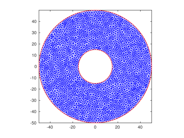
Figure 5.1: Mesh of the Schnakenberg model.

Specifying the chemical reactions

We readily construct the propensity file using the utility-function rparse:

r1 = ’@ > k1*vol > U’;
r2 = ’U > k2*U > @’;
r3 = ’@ > k3*vol > V’;
r4 = ’U+U+V > (k4/(vol*vol))*(U*(U-1)*V) > U+U+U’;
umod = rparse(umod,{r1 r2 r3 r4},{’U’ ’V’}, ...
         {’k1’ 0.1 ’k2’ 1 ’k3’ 0.9 ’k4’ 1}, ...
         ’schnakenberg.c’);

The result of the above command is written on the indicated file. Take a moment to study the resulting source code!

We also need to define a few more fields of the umod-struct:

umod.u0 = zeros(size(umod.N,1),numel(umod.vol));
umod.tspan = 0:10:100;
umod.vol = 50/mean(umod.vol)*umod.vol;

The last command is special to the current model: it is of some interest to investigate how the Schnakenberg model responds to different scaling of the system volume. Here this is achieved by directly rescaling the field vol of the umod-struct.

Simulating the model

At this stage we simply invoke urdme:

umod = urdme(umod,’report’,3);

! Using report = 3 implies that you have the possibility to discontinue the simulation at each entry in tspan. A useful feature when setting up new models.

Postprocessing

To use PDE Toolbox in the visualization process we rely on the function urdme2pde:

umod = urdme2pde(umod);
figure, clf,
pdesurf(umod.pde.P,umod.pde.T,umod.pde.U(1,:,end)’);
title(’Schnakenberg: Concentration U’);
view(0,90), axis tight, axis square, colormap(’parula’)

The result of these plot-commands can be inspected by running the example. In the file morphogenesis2D_run.m a second model, the Brusselator, is also solved in a similar fashion.

5.2 Min oscillations in E. Coli

To illustrate the solution steps in a more advanced 3D model, we will reproduce simulations of the Min-system from [21]. The geometry will be a model of an E. coli bacterium. It is rod-shaped with length $3.5\mu m$ and diameter $0.5\mu m$. The reactions and parameters of the model can be found in Table 5.1. The model is built in the file mincde_run.m found in the folder ‘examples/mincde’.

$\mbox{MinDcytATP}\xrightarrow{k_{d}}\mbox{MinDmem}$	$\mbox{MinDcytATP}+\mbox{MinDmem}\xrightarrow{k_{dD}}\mbox{2MinDmem}$
$\mbox{MinE+MinDmem}\xrightarrow{k_{de}}\mbox{MinDE}$	$\mbox{MinDE}\xrightarrow{k_{e}}\mbox{MinDcytADP}+\mbox{MinE}$
$\mbox{MinDcytADP}\xrightarrow{k_{p}}\mbox{MinDcytATP}$

Table 5.1: The chemical reactions of the Min system. The constants take the values $k_{d}=0.0125\mu m^{-1}s^{-1}$, $k_{dD}=9\times 10^{6}M^{-1}s^{-1}$, $k_{de}=5.56\times 10^{7}M^{-1}s^{-1}$, $k_{e}=0.7s^{-1}$, and $k_{p}=0.5s^{-1}$.

5.2.1 Setting up the model for simulation

Defining the geometry and diffusion rates in Comsol Multiphysics

1. Open Comsol and use the Model Wizard to create the model template. Select ‘3D’ as space dimension and add the physics module ‘Chemical Species Transport / Transport of Diluted Species’ in the next step. In the ‘Dependent variables’ window chose the ‘Number of species’ to be 5 and in the ‘Concentrations’ list enter the names MinDcytATP, MinDmem, MinE, MinDE and MinDcytADP. You may also enter these variable names at a later stage, see below. Select the ‘Time Dependent’ study type in the next step of the wizard and click on the flag symbol to create the template.

   ! Note that the ‘Chemical engineering module’ is not required in general for URDME, but is used in this example for convenience.

2. Next we create the geometry. We will build the rod shaped domain from two spheres and one cylinder. Right click on ‘Geometry 1’, select the ‘Cylinder’ option and in the radius and height field enter 0.5e-6 and 3.5e-6. Click on the ‘Build Selected’ Button and you should now see a cylinder in your workspace. Now, select the ‘Sphere’ node from the ‘Geometry’ context-menu and and enter 0.5e-6 in the radius field. Create another identical sphere but enter 3.5e-6 as the $x$-coordinate. Click on ‘Build All’ and observe the created domain in the graphics-window.

   Right click on ‘Geometry’ again and select ‘Boolean Operations $>$ Union’. Select all three domains and add them to the ‘Input objects’ selection. Uncheck the ‘Keep interior boundaries’ box and complete the geometry creation by pushing the ‘Build All’ button. The final geometry has 1 domain, 12 boundaries, 20 edges, and 10 vertices.

3. Having constructed the geometry, the next step is to specify the parameters in the model. If you haven’t specified the variable names yet, do this now under ‘Transport of Diluted Species $>$ Dependent Variables’ (Number of species: 5, Concentrations: MinDcytATP, MinDmem, MinE, MinDE, MinDcytADP).

   In the physics settings ‘Transport of Diluted Species $>$ Transport Mechanisms’, deactivate the flag on ‘Convection’. Also, with the ‘Transport of Diluted Species’ tab active, press the advanced property icon (an all-seeing eye just under the ‘Model Builder’ title), and select ‘Discretization’. Use linear elements and uncheck the ‘Compute boundary fluxes’.

   Next we need to specify the diffusion constants of the species in the ‘Diffusion’ node of the physics menu ‘Transport Properties’. Enter the diffusion coefficients 2.5e-12 for MinDcytATP, MinE, and MinDcytADP. For MinDE and MinDmem the diffusion constant should be 1e-14. The units of all constants are $m^{2}/s$.

   ! MinDE and MinDmem are species bound to the membrane, hence their lower diffusion rates. We have not specified this explicitly at this stage, but will do so later in the Matlab layer.

4. In order to be able to distinguish between the interior of the bacterium and the membrane, we must also create two domains which URDME can parse. One interior domain that represents the cytoplasm and one boundary domain that represents the membrane. This is done by (1) defining the global urdme_sdlevel variable, and (2) defining the variable urdme_sd on the geometry as an expression with different values in the different subdomains. The latter variable is then used by URDME to distinguish the nodes on the boundary from those in the interior. Somewhat technically, the former variable, urdme_sdlevel, is required to correctly evaluate the value of urdme_sd on the different manifolds of the model (points, edges, boundaries, domain).

   First click right on ‘Global Definitions’ and create the ‘Variable’ urdme_sdlevel. Assign this variable the value 2 to indicate that the lowest dimension where urdme_sd is defined is on the boundaries of the geometry (where the dimensionality is 2).

   Second, click right on the menu ‘Definitions’, and create two ‘Variables’. Label the first one urdme_sd_dom (name is not critical) and select the ‘Geometry entity level’ to be ‘Domain’ and chose the ‘Selection’ to be ‘All domains’. Now, enter a new variable in the window below by specifying the name to urdme_sd and expression to 1. Similarly, label the second variable urdme_sd_bnd (again, name is not critical), specify the geometric entity level to ‘Boundary’ and set the ‘Selection’ to ‘All boundaries’. Enter the variable name urdme_sd into the ‘Variables’ window and set the expression to 2.

   All in all we have now defined the variable urdme_sdlevel to be 2 globally such that URDME will correctly evaluate the variable urdme_sd first at the entire domain of the model (where urdme_sd = 1) and second at the boundaries of the model (where urdme_sd = 2). The URDME convention here is that lower dimensional manifolds take precedence over higher dimensional ones.

5. In the ‘Mesh’ node, set ‘User controlled mesh’ as sequence type and in the appeared ‘Size’ node select the ‘Custom’ option. Set the maximum element size to 1e-7 and press ‘Build All’. Now click on the ‘Study’ node and press the ‘Compute’ button.

6. Some Comsol callback functions require a placeholder solution. To create a simple such solution, under ‘Study 1: Time Dependent’, select ‘Times: range(0,1,1)’ and press the ‘Compute’ button.

Now you need to transfer the created model into Matlab. Make sure that you are connected to the Server, if not, connect via ‘File $>$ Client Server $>$ Connect to Server’. When having a working connection the export can be performed by selecting ‘File $>$ Client Server $>$ Export Model to Server’.

Another option is to save the model to file (here: coli.mph), and open it later in a running Matlab session with ‘LiveLink’ via the command mphload:

model = mphload(’coli.mph’); % load Comsol model
umod = comsol2urdme(model);  % create URDME struct

Specifying the chemical reactions

The chemical reactions are specified in a separate file written in C, conveniently generated on the fly by the utility function rparse. Open the file ‘examples/mincde/mincde_run.m’. We will walk through the contents of this file and explain what the different parts do. Additional information can also be found in the comments in the file.

First out is the membrane bound reaction,

r1 = ’MinDcytATP > sd == 2 ? kd*MinDcytATP/ldata[0] : 0.0 > MinDmem’;

Note how sd is used to check if the voxel belongs to the membrane or not. We have to make sure, however, that we keep track of what value we assigned to the different subdomains in the Comsol model file (the value of the expression urdme_sd).

Note also how the first reaction in the model contains a scaling with the local length scale of the subvolume. For a uniform Cartesian mesh this would simply have been the (constant) side lengths of the cubes in the mesh. For the unstructured mesh however, this value will be different in every subvolume. It is readily obtained from Comsol, and is passed to the propensity function via the data vector ldata which will be initialized with the correct values below.

We continue with the two bimolecular reactions,

r2 = [’MinDcytATP + MinDmem > kdD*MinDcytATP*MinDmem/(1000.0*NA*vol)’ ...
      ’> MinDmem+MinDmem’];
r3 = ’MinE + MinDmem > kde*MinE*MinDmem/(1000.0*NA*vol) > MinDE’;

Note the unit conversions given explicitly in the bimolecular propensity function. The rate constants for the bimolecular reactions in this model are given in the unit $M^{-1}s^{-1}$ and need to be converted to mesoscopic rates. That is why we divide with Avogadros number times the volume of the subvolume. Also, the way we have set up the geometry model file, the volume is given in the unit $m^{3}$, and needs to be converted to $L^{3}$. URDME cannot keep track of matching the units between the different model files automatically: this is the responsibility of the end-user.

The chemical network is concluded with two degradation reactions:

r4 = ’MinDE > ke*MinDE > MinDcytADP + MinE’;
r5 = ’MinDcytADP > kp*MinDcytADP > MinDcytATP’;

To create the propensity file we define the species and the rate constants and then invoke rparse:

species = {’MinDcytATP’ ’MinDmem’ ’MinE’ ’MinDE’ ’MinDcytADP’};
rates = {’NA’ 6.022e23 ’kd’ 1.25e-8 ’kdD’ 9.0e6 ’kde’ 5.56e7 ...
         ’ke’ 0.7 ’kp’ 0.5};
umod = rparse(umod,{r1 r2 r3 r4 r5},species,rates,’fange.c’);

The propensity C-file is now found in the file fange.c. Take a moment to study this file!

Before we can run the simulation, we need to modify the diffusion rates that we obtain from the initial Comsol model so that the membrane-bound species only diffuse on the membrane. We have already prepared for this by labeling the subvolumes next to the boundary using the expression urdme_sd in the Comsol model.

1. The initial condition. There is complete freedom in specifying the initial condition. In the present case we simply distribute 4002 MinDcytATP and 1040 MinE molecules in some random way in the entire bacterium.

   % the total number of molecules of the species
   nMinD = 4002;
   nMinE = 1040;
   
   % assign randomly
   u0 = zeros(Mspecies,Ncells);
   ind = floor(Ncells*rand(1,nMinE))+1;
   u0(3,:) = full(sparse(1,ind,1,1,Ncells));
   ind = floor(Ncells*rand(1,nMinD))+1;
   u0(5,:) = full(sparse(1,ind,1,1,Ncells));
   umod.u0 = u0;
   

   Note that the code above does not produce a uniformly random initial distribution since the volume of each voxel is not taken into account.

2. Specifying the times to output the state of the system. URDME will look for a vector tspan to determine when to output the state of the trajectory (the number of events generated in a typical realization often exceeds $10^{9}$ so we can’t output after each event). Here, we want to sample the system on the time interval $[0,200]$ seconds, with output each second. This is achieved by

   umod.tspan = 0:200.
   

3. Membrane diffusion. In order to make MinDmem and MinDE diffuse only on the membrane, we will zero out all elements in the diffusion matrix that are in the cytosol. To obtain indices of those subvolumes we use the information in the subdomain vector sd.

   cyt = find(umod.sd == 1);
   pm  = find(umod.sd == 2);
   

   Remember that we gave urdme_sd the value 2 on the membrane and 1 in the interior. The diffusion matrix D will contain the rate constants for the diffusive events on the unstructured mesh. D is generated by Comsol and is available in the field umod.D. To (efficiently) zero out the correct entries in D, we first decompose the sparse matrix, find the entries using pm and cyt above, and then reassemble the matrix again (compensating for the removed entries by adjusting the diagonal of the matrix). All in all, the code to do this is as follows:

   % For MinDmem (2) and MinDE (4), flag all dofs in the cytosol for
   % removal.
   ixremove = [];
   for s = [2 4]
     ixremove = [ixremove; Mspecies*(cyt-1)+s];
   end
   
   % Decompose the sparse matrix.
   D = umod.D’;
   [i,j,s] = find(D);
   
   % Set all elements in the diffusion matrix corresponding
   % to the cytosol to zero.
   ixremove = [find(ismember(i,ixremove)); find(ismember(j,ixremove))];
   i(ixremove) = [];
   j(ixremove) = [];
   s(ixremove) = [];
   
   % Reassemble the sparse matrix and adjust the diagonal entries.
   ixkeep = find(s > 0);
   D = sparse(i(ixkeep),j(ixkeep),s(ixkeep),Ndofs,Ndofs);
   d = full(sum(D,2));
   D = D+sparse(1:Ndofs,1:Ndofs,-d);
   umod.D = D’;
   

   ! It is of fundamental importance that the columns of D sum to zero, and that all off-diagonal entries are positive. For an introduction to how D is constructed, see Appendix A. For a detailed account, consult [17].

   ! The way we have modeled membrane diffusion is simply by saying that the subvolumes closest to the membrane constitute the membrane layer. As the mesh becomes finer near the boundary, the thickness of this layer will decrease, eventually approaching a 2D model of the membrane. One can also think of other ways of modeling the membrane diffusion.

4. The local data vector. Finally, we need to set umod.ldata to contain the values of the length parameter for the subvolumes (it is needed in the first reaction). To do this, we use the built-in Comsol function mphinterp which can be used to evaluate an expression in any point in the domain. Here, we simply get the subvolume sizes by using the pre-defined expression h, evaluated in the vertices of the mesh.

   Relying on Comsol Multiphysics:

   xmi = mphxmeshinfo(umod.comsol);
   umod.ldata = mphinterp(umod.comsol,’h’,’coord’, ...
                          xmi.dofs.coords(:,1:Mspecies:end),’solnum’,1);
   umod.ldata = umod.ldata(xmi.dofs.nodes(1:Mspecies:end)+1);
   

   ! For more details concerning the internal ordering of the dofs, consult the Comsol user’s manual. The interface routines comsol2urdme and urdme2comsol also contain useful information on this matter.

5.2.2 Running the simulation

With the model set up correctly, we are now ready to simulate:

umod = urdme(umod,’report’,2);

URDME will now compile the solver with linking to the propensities specified in fange.c, and then execute the solver. The result of the simulation is stored in umod.U. To prepare for post-processing we can transfer this result back to the Comsol object,

umod = urdme2comsol(umod);

5.2.3 Post-processing

If the simulation in the previous step completed without errors, the model structure will now contain a realization of the stochastic process. To visualize the trajectory, we can use any of the visualization options available in Comsol or we can create routines of our own. To look at the MinDmem distribution on the membrane at the final time we can use Comsol’s post-processing functionality.

This command creates a plot-container for the visualization to follow:

umod.comsol.result.create(’res1’,’PlotGroup3D’);

To visualize the result at a specific time, e.g., after 100s:

umod.comsol.result(’res1’).set(’t’,’100’);

! You can specify any time in the interval you simulated, but if you specify a time that lies between two points in tspan Comsol will do interpolation to approximate the result at that point.

To visualize the result of the simulation on the surface we can use:

umod.comsol.result(’res1’).feature.create(’surf1’,’Surface’);
umod.comsol.result(’res1’).feature(’surf1’).set(’expr’,’MinDmem’);
mphplot(umod.comsol,’res1’);

Where we can replace the string ’MinDmem’ with the name of any other species.

To visualize the solution inside the domain, we need to first create a new plot container.

umod.comsol.result.create(’res2’,’PlotGroup3D’);
umod.comsol.result(’res2’).set(’t’,’100’);

Now we can visualize the solution on a ‘slice’ of the $zx$-axis of the model.

umod.comsol.result(’res2’).feature.create(’slc2’,’Slice’);
umod.comsol.result(’res2’).feature(’slc2’).set(’expr’,’MinDcytATP’);
umod.comsol.result(’res2’).feature(’slc2’).set(’quickplane’,’zx’);
umod.comsol.result(’res2’).feature(’slc2’).set(’quickynumber’,’1’);
mphplot(model,’res2’);

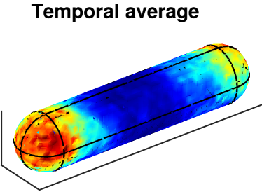
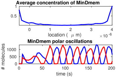
Figure 5.2: Visualizations from the Min system.

There are many more options that can be passed to mphplot to control the plot produced. For a detailed account, see the Comsol documentation:

>> help mphplot

If you prefer to work within the Comsol GUI for visualization, you can import back the Comsol model with the attached stochastic trajectory into Comsol. This can be done by typing:

>> mphsave(umod.comsol,’<output_filename>.mph’)

Optionally, from the Comsol GUI, import the new structure (umod.comsol): ’File $>$ Client Server $>$ Import Model from Server’. You can now visualize the trajectory using the options provided in the ‘Results’ node.

6 Integrating solvers with URDME

URDME is easily enriched with additional third party solvers. URDME plugins have three main components: the mex-based makefile, the mex-interface source code, and (conventionally) a placeholder Matlab .m-file with defining help-text. Each part is described in Table 6.1 where the files that make up the NSM solver are explained. We recommend that developers follow this format when integrating their own solvers.

File	Description
mexmake_nsm.m	A mex-based makefile for building the solver. The name of this file is important: the automatic compilation process looks for a makefile that is suffixed with the name of the solver. This makefile compiles the solver with the model’s propensity functions into the executable mexnsm which is called by the Matlab-level interface.
mexnsm.c	Solver entry point, a mexFunction.
nsm.h, nsm.c	Actual low-level source code implementing the NSM solver.
nsm.m	Empty Matlab .m-file containing help-text.

Table 6.1: Overview of the files that make up the NSM solver.

Appendix A Stochastic chemical kinetics

In this section we briefly describe how reaction and diffusion events are modeled and how we obtain the diffusion rate constants when the domain is discretized using an unstructured mesh. For a more detailed introduction to the subject along with many additional references, consult, e.g., [13].

The computational core of URDME is based on the next subvolume method (NSM) [10]. Details concerning the actual simulation algorithms can be found in Appendix B.

A.1 Mesoscopic chemical kinetics

In a well-stirred chemical environment reactions are understood as transitions between the states of the integer-valued state space counting the number of molecules of each of $D$ different species. The intensity of a transition is described by a reaction propensity defining the transition probability per unit of time for moving from the state $x$ to $x+N_{r}$;

$$x \xrightarrow{\omega_{r}(x)}x+N_{r},$$ (A.1)

where $N_{r}\in\mathbf{Z}^{D}$ is the transition step and is the $r$th column in the stoichiometric matrix $N$. Eq. (A.1) defines a continuous-time Markov chain over the positive $D$-dimensional integer lattice.

When the reactions take place in a container of volume $\Omega$, it is sometimes useful to know that the propensities often satisfy the simple scaling law

$$\omega_{r}(x) =\Omega u_{r}(x/\Omega)$$ (A.2)

for some function $u_{r}$ which does not involve $\Omega$. Intensities of this form are called density dependent and arise naturally in a variety of situations [20, Ch. 11].

A.2 Mesoscopic diffusion

In the mesoscale model, a diffusion event is modeled as a first order reaction taking species $S_{l}$ in subvolume $\zeta_{i}$ from its present subvolume to an adjacent subvolume $\zeta_{j}$,

$$S_{li}\xrightarrow{a_{ij}\mathbf{x}_{li}}S_{lj},$$ (A.3)

where $\mathbf{x}_{li}$ is the number of molecules of species $l$ in subvolume $i$. On a uniform Cartesian mesh such as those used in MesoRD [27], the rate constant takes the value $a_{ij}=\gamma/h^{2}$ where $h$ is the side length of the subvolumes and $\gamma$ is the diffusion constant. In URDME we use an unstructured mesh made up of tetrahedra and the rate constants are taken such that the expected value of the number of molecules divided by the volume (the concentration) converges to the solution obtained from a consistent FEM discretization of the diffusion equation

$$u_{t}=\gamma\Delta u.$$ (A.4)

Using piecewise linear Lagrange elements and mass lumping, we obtain the discrete problem

$$u_{t}=M^{-1}Ku$$ (A.5)

where $M$ is the lumped mass matrix and $K$ is the stiffness matrix. The rate constants on the unstructured mesh are then given by

$$a_{ij}=\frac{1}{\Omega_{i}}k_{ij},$$ (A.6)

where $\Omega_{i}$ is the diagonal entry of $M$ and can be interpreted as the volume of the dual element associated with mesh node $i$ (see Figure A.1). For more details, consult [17].

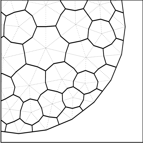
Figure A.1: A 2D example of an unstructured triangular mesh. The primal mesh is shown in dashed and the dual in solid. Within each dual element the system is assumed to be well-stirred, and molecules can jump from each dual cell to the neighboring ones.

The assumption made in the mesoscopic model is that molecules are well-stirred within a dual cell. These dual cells correspond to the cubes of the staggered grid in a Cartesian mesh.

Appendix B Algorithms

One of the most popular algorithms to generate realizations of the CTMC in the well-stirred case is Gillespie’s direct method (DM) [24]. Several algorithmic improvements of this method exist, one of them being the next reaction method (NRM) due to Gibson and Bruck [23].

The underlying algorithm in URDME is the next subvolume method (NSM) [10]. The NSM can be understood as a combination of NRM and DM in order to tailor the algorithm to reaction-diffusion processes.

For reference, we first state below both DM and NRM and then outline NSM.

Algorithm 1 Gillespie’s direct method (DM)

  Initialize: Set the initial state $\mathbf{x}$ and compute all propensities $\omega_{r}(\mathbf{x}),r=1,\ldots,M_{\mbox{\footnotesize{reactions}}}$. Also set $t=0$.

  while $t<T$ do

     Compute the sum $\lambda$ of all the propensities.

     Sample the next reaction time (by inversion), $\tau=-\log(\mbox{rand})/\lambda$. Here and in what follows, ‘rand’ conveniently denotes a uniformly distributed random number in $(0,1)$ which is different for each occurrence.

     Sample the next reaction event (by inversion); find $n$ such that
$\sum_{j=1}^{n-1}\omega_{j}(\mathbf{x})<\lambda\,\mbox{rand}\leq\sum_{j=1}^{n}\omega_{j}(\mathbf{x})$

     Update the state vector, $\mathbf{x}=\mathbf{x}+N_{n}$ and set $t=t+\tau$.

  end while

Algorithm 2 Gibson and Bruck’s next reaction method (NRM)

  Initialize: Set $t=0$ and assign the initial number of molecules. Generate the dependency graph $G$. Compute the propensities $\omega_{r}(\mathbf{x})$ and generate the corresponding absolute waiting times $\tau_{r}$ for all reactions $r$. Store those values in a heap $H$.

  while $t<T$ do

     Remove the smallest time $\tau_{n}=H_{0}$ from the top of $H$, execute the $n$th reaction $\mathbf{x}:=\mathbf{x}+N_{n}$ and set $t:=\tau_{n}$.

     for all edges $n\to j$ in $G$ do

        if $j\not=n$ then

           Recompute the propensity $\omega_{j}$ and update the corresponding waiting time according to

$$\tau_{j}^{\mathrm{new}} =t+\left(\tau_{j}^{\mathrm{old}}-t\right)\frac{\omega_{j}^{\mathrm{old}}}{\omega_{j}^{\mathrm{new}}}.$$

        else {$j=n$}

           Recompute the propensity $\omega_{n}$ and generate a new absolute time $\tau_{n}^{\mathrm{new}}$. Adjust the contents of $H$ by replacing the old value of $\tau_{n}$ with the new one.

        end if

     end for

  end while

Algorithm 3 The next subvolume method (NSM)

  Initialize: Compute the sum $\sigma_{i}^{r}$ of all reaction rates $\omega_{ri}$ and the sum $\sigma_{i}^{d}$ of all diffusion rates $a_{ij}\mathbf{x}_{si}$ in all subvolumes $i=1,\ldots,N_{\mbox{\footnotesize{cells}}}$. Compute the time until the next event in each subvolume, $\tau_{i}=-\log(\mbox{rand})/(\sigma_{i}^{r}+\sigma_{i}^{d})$, and store all times in a heap $H$.

  while $t<T$ do

     Select the next subvolume $\zeta_{n}$ where an event takes place by extracting the minimum $\tau_{n}$ from the top of $H$.

     Set $t=\tau_{n}.$

     Determine if the event in $\zeta_{n}$ is a reaction or a diffusion event. Let it be a reaction if $(\sigma_{n}^{r}+\sigma_{n}^{d})\,\mbox{rand}<\sigma_{n}^{r}$, otherwise it is a diffusion event.

     if Reaction event then

        Determine the reaction channel that fires. This is done by inversion of the distribution for the next reaction given $\tau_{n}$ in the same manner as in Gillespie’s direct method in Algorithm 1.

        Update the state matrix using the (sparse) stoichiometric matrix $N$.

        Update $\sigma_{n}^{r}$ and $\sigma_{n}^{d}$ using the dependency graph $G$ to recalculate only affected reaction- and diffusion rates.

     else {Diffusion event}

        Determine which species $S_{ln}$ diffuses and subsequently, determine to which neighboring subvolume $\zeta_{n^{\prime}}$. This is again done by inversion using a linear search in the corresponding column of $D$.

        Update the state: $S_{nl}=S_{nl}-1$, $S_{n^{\prime}l}=S_{n^{\prime}l}+1$.

        Update the reaction- and diffusion rates of subvolumes $\zeta_{n}$ and $\zeta_{n^{\prime}}$ using G.

     end if

     Compute a new waiting time $\tau_{n}$ by drawing a new random number and add it to the heap $H$.

  end while

References

- [1] N. Barkai and S. Leibler. Circadian clocks limited by noise. Nature, 403:267–268, 2000.
- [2] P. Bauer and S. Engblom. Sensitivity estimation and inverse problems in spatial stochastic models of chemical kinetics. In A. Abdulle, S. Deparis, D. Kressner, F. Nobile, and M. Picasso, editors, Numerical Mathematics and Advanced Applications: ENUMATH 2013, volume 103 of Lecture Notes in Computational Science and Engineering, pages 519–527, Berlin, 2015. Springer.
- [3] P. Bauer and S. Engblom. The URDME manual version 1.3. Technical report, Dept of Information Technology, Uppsala University, 2017. Available at http://arxiv.org/abs/0902.2912.
- [4] P. Bauer, S. Engblom, S. Mikulovic, and A. Senek. Multiscale modelling via split-step methods in neural firing. Math. Comput. Model. Dyn. Syst., 24(4):409–425, 2018.
- [5] E. Blanc, S. Engblom, A. Hellander, and P. Lötstedt. Mesoscopic modeling of stochastic reaction-diffusion kinetics in the subdiffusive regime. Multiscale Model. Simul., 14(2):668–707, 2016.
- [6] Y. Cao, D. T. Gillespie, and L. Petzold. Multiscale stochastic simulation algorithm with partial equilibrium assumption for chemically reacting systems. J. Comput. Phys., 206:395–411, 2005.
- [7] Comsol Inc. Comsol Multiphysics Reference Guide, 5.2 edition, 2017.
- [8] B. Drawert, S. Engblom, and A. Hellander. URDME: a modular framework for stochastic simulation of reaction-transport processes in complex geometries. BMC Syst. Biol., 6(76):1–17, 2012.
- [9] W. E, D. Liu, and E. Vanden-Eijnden. Nested stochastic simulation algorithm for chemical kinetic systems with disparate rates. J. Chem. Phys., 123, 194107, 2005.
- [10] J. Elf and M. Ehrenberg. Spontaneous separation of bi–stable biochemical systems into spatial domains of opposite phases. Syst. Biol., 1(2), 2004.
- [11] M. B. Elowitz, A. J. Levine, E. D. Siggia, and P. S. Swain. Stochastic gene expression in a single cell. Science, 297(5584):1183–1186, 2002.
- [12] S. Engblom. Computing the moments of high dimensional solutions of the master equation. Appl. Math. Comput., 180(2):498–515, 2006.
- [13] S. Engblom. Numerical Solution Methods in Stochastic Chemical Kinetics. PhD thesis, Uppsala University, 2008.
- [14] S. Engblom. Galerkin spectral method applied to the chemical master equation. Commun. Comput. Phys., 5(5):871–896, 2009.
- [15] S. Engblom. Spectral approximation of solutions to the chemical master equation. J. Comput. Appl. Math., 229(1), 2009.
- [16] S. Engblom. Stochastic simulation of pattern formation in growing tissue: a multilevel approach. Bull. Math. Biol., 81:3010–3023, 2019.
- [17] S. Engblom, L. Ferm, A. Hellander, and P. Lötstedt. Simulation of stochastic reaction–diffusion processes on unstructured meshes. SIAM J. Scientific. Comp., 31(3):1774–1797, 2009.
- [18] S. Engblom, P. Lötstedt, and L. Meinecke. Mesoscopic modeling of random walk and reactions in crowded media. Phys. Rev. E, 98(3):033304, 2018.
- [19] S. Engblom, D. B. Wilson, and R. E. Baker. Scalable population-level modelling of biological cells incorporating mechanics and kinetics in continuous time. Roy. Soc. Open Sci., 5(8), 2018.
- [20] S. N. Ethier and T. G. Kurtz. Markov Processes: Characterization and Convergence. Wiley series in Probability and Mathematical Statistics. John Wiley & Sons, New York, 1986.
- [21] D. Fange and J. Elf. Noise-induced Min phenotypes in E. coli. PLOSB, 2(6):0637–0647, 2006.
- [22] L. Ferm and P. Lötstedt. Adaptive solution of the master equation in low dimensions. Appl. Numer. Math., 59(1):265–284, 2009.
- [23] M. A. Gibson and J. Bruck. Efficient exact stochastic simulation of chemical systems with many species and many channels. J. Phys. Chem., 104:1876–1889, 2000.
- [24] D. T. Gillespie. A general method for numerically simulating the stochastic time evolution of coupled chemical reacting systems. J. Comput. Phys., 22:403–434, 1976.
- [25] D. T. Gillespie. Approximate accelerated stochastic simulation of chemically reacting systems. J. Chem. Phys., 115(4):1716–1733, 2001.
- [26] E. L. Haseltine and J. B. Rawlings. Approximate simulation of coupled fast and slow reactions for stochastic chemical kinetics. J. Chem. Phys., 117(15):6959–6969, 2002.
- [27] J. Hattne, D. Fange, and J. Elf. Stochastic reaction–diffusion simulation with MesoRD. Bioinformatics, 21(12):2923–2924, 2005.
- [28] M. Hegland, C. Burden, L. Santoso, S. MacNamara, and H. Booth. A solver for the stochastic master equation applied to gene regulatory networks. J. Comput. Appl. Math., 205(2):708–724, 2007.
- [29] A. Hellander and P. Lötstedt. Hybrid method for the chemical master equation. J. Comput. Phys., 227(1):127–151, 2008.
- [30] S. F. MacNamara. Krylov and Finite State Projection Methods for Simulating Stochastic Biochemical Kinetics via the Chemical Master Equation. PhD thesis, The University of Queensland, Australia, 2008.
- [31] The Mathworks Inc. Partial Differential Equation Toolbox, 2.3 edition, 2017.
- [32] H. H. McAdams and A. Arkin. It’s a noisy business! Genetic regulation at the nanomolar scale. Trends in Genetics, 15(2):65–69, 1999.
- [33] J. Paulsson, O. G. Berg, and M. Ehrenberg. Stochastic focusing: Fluctuation-enhanced sensitivity of intracellular regulation. Proc. Nat. Acad. Sci. USA, 97(13):7148–7153, 2000.
- [34] C. V. Rao and A. P. Arkin. Stochastic chemical kinetics and the quasi-steady-state assumption: Application to the Gillespie algorithm. J. Chem. Phys., 118(11):4999–5010, 2003.
- [35] Y. Saygun. Computational stochastic morphogenesis. Master’s thesis, Uppsala University, 2015. UPTEC F15 041.
- [36] M. Thattai and A. van Oudenaarden. Intrinsic noise in gene regulatory networks. Proc. Nat. Acad. Sci. USA, 98:8614–8619, 2001.