Chaos at Nonlinear NMR

Abstract

The hodographs of magnetization of nonlinear NMR are investigated in the conditions of resonance on the unshifted frequency. It is shown that, depending on the value of amplitude of the variable field and value of frequency shift, topologically different hodographs separated from each other by separatrix are obtained. It is shown that the set of hodograph points, being obtained by the stroboscopic method, is chaotic and the change of $z$-component of magnetization has the form of solitons chaotically changing the sign.

1 Introduction

Investigations of nonlinear magnetic resonance in magnetically ordered materials have been carried out for a long time [1], however the interest to them is still increasing due to discovery of new physical phenomena in magnetics [2–9]. On the other hand the interest to chaotic Hamiltonian systems does not weaken [10–12]. That is why the study of any questions on the butt of these two fields (our work concerns to) in our opinion is quite topical. In particular most of spin systems considered as promising candidates for applications in quantum computation are nonlinear [13–17]. Nonlinearity is a principle problem for controlled states. Note that for a linear system in a constant magnetic field, magnetization vector can be deflected by applying a variable radio frequency field. However for nonlinear systems, situation is completly different.

In magnetically ordered crystals at quite, low temperatures a shift of frequency precession of nuclear magnetization ${\bf m}$ proportional to the longitudinal component $m_{z}$ (dynamical shift) origins. In the NMR conditions appearance of dynamic shift leads to essentially nonlinear character of the motion ${\bf m}$. For example, in [18] it was shown, that fulfilling the conditions $\omega_{1}=\omega_{p}$, where $\omega_{p}$ is equilibrium value of dynamic shift, $\omega_{1}=\eta\gamma H_{1},~{}H_{1}$ is an amplitude of linearly polarized variable field, applied in the transverse plane, $\eta$ is gain factor, $\gamma$ is a gyromagnetic ratio, the motion of ${\bf m}$ vector in the rotational coordinate system becomes aperiodic (period $T\rightarrow\infty$). Trajectory, along which the end of ${\bf m}$ vector moves (hodograph) in this case is a separatrix topologically separating differing trajectories. It will be shown below that points put according to hodograph being close to separatrix form a stochastic set. Simple, but effective method of finding the stochastic motion (stroboscopic method) is offered.

Peculiarity of dynamical systems is extreme sensitivity of motion near separatrix, even with respect to the slightly change of initial conditions or adiabatic perturbation. Purpose of our paper is demonstration at the fact that control of the state of nonlinear system is not possible near separatrix. In order to proof this statement, we shall consider realistic physical system. Namely, we shall study motion of nuclear magnetization in the presence of large dynamical shift of frequency.

2 Equations of motion of magnetization at nonlinear NMR

Let us direct the axis z along the total field ${\bf H}={\bf H}_{0}+{\bf H}_{loc}$, where ${\bf H}_{0}$ and ${\bf H}_{loc}$ are respectively external and internal magnetostatic fields on the nuclei. Let us assume that the variable fields also effect on the nuclear spin-system

$${\bf H}_{1}(t)={\bf H}_{1}\cos\omega t,~{}~{}~{}{\bf H}_{1}\perp{\bf H}$$ (1)

and

$${\bf h}_{1}(t)={\bf h}_{1}\cos\nu t,~{}~{}~{}{\bf h}\parallel{\bf H}$$ (2)

Directing ${\bf H}_{1}$ along the axis $x$, the system of nonlinear differential equations describing the motion of nuclear magnetization with the account of dynamical shift of frequency precession in the rotating system of coordinates around the axis $z$ with the frequency can be written as follows

$$\dot{x}=(\Delta-\omega_{p}z)y+\nu_{1}y\cos\nu t,$$

$$\dot{y}=-(\Delta-\omega_{p}z)x+\frac{1}{2}\omega_{1}z-\nu_{1}x\cos\nu t,$$ (3)

$$\dot{z}=-\frac{1}{2}\omega_{1}y,~{}~{}\nu_{1}=\gamma h,~{}~{}\Delta=\omega-\omega_{0},~{}~{}\omega_{0}=\gamma H.$$

Here we introduced dimensionless components of magnetization $\alpha=m_{\alpha}/m,$ where $m=|{\bf m}|,~{}\alpha=x,y,z.$ Our observation neglects relaxation effects and magnetostatic inhomogeneity of the local field is valid in the case of fields with duration $\tau\ll T_{1},~{}T_{2},~{}2\pi/\Omega,$ where $T_{1}$ and $T_{2}$ are the times of longitudinal and transverse relaxation, $\Omega$ is inhomogeneous width of the line. The system (3) is investigated in the conditions of weakness of longitudinal fields $(\nu_{1}\ll\omega_{p}).$

We investigate an unperturbed system being obtained from (3) at $\nu_{1}=0.$ It is easy to see that unperturbed system has two integrals of motion:

$$x^{2}+y^{2}+z^{2}=1$$ (4)

$$\omega_{p}z^{2}-\omega_{1}x=\omega_{p}.$$ (5)

The first of these integrals (4) corresponds to conservation of the value of full magnetic moment, the second (5) corresponds to the conservation of full magnetic energy. Here we assume that the conditions of resonance are fulfilled on the unshifted frequency $\Delta=0,$ and $x(0)=y(0)=0,~{}z(0)=1$ are taken as initial conditions. These relations give definite surfaces: (4) single sphere and (5) parabolic cylinder with generatrix along the axis $y$. Hodographs of vector ${\bf m}$ are closed curves obtained by crossing of these surfaces.

When $\omega_{1}\neq\omega_{p}$, hodographs are divided into two types: 1) $\omega_{1}<\omega_{p}$ - the section consists of two contours, which are symmetrically located on different sides of the plane $(x,y)$; 2) $\omega_{1}>\omega_{p}$ - the section consists of one contour twice crossing the plane $(x,y)$. When $\omega_{1}=\omega_{p}$ the trajectory looks like symmetrical spatial eight with self-crossing on the axis $x$, at $x=-1$ (Fig.1). One-parametric (parameter $\omega_{1}$) family of eights creates the separatrix of unperturbed motion, which divides the space into domains according to the type of their trajectories.

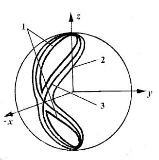
Figure 1: Family of hodographs of vector ${\bf r}={\bf m}/|m_{0}|$ in the conditions of resonance on the unshifted frequency: 1) $\omega_{1}<\omega_{p}$. Two closed curves, located symmetrically relatively to the plane $(x,y)$. 2) $\omega_{1}>\omega_{p}$. The curve looks like the spatial eight, which crosses the plane $(x,y)$ twice. 3) $\omega_{1}=\omega_{p}$. The spatial eight with self-crossing on the axis$x$ at $x=-1$ acts as separatrix.

Using the integrals of motion (4) and (5) unperturbed $(\nu_{1}=0)$ system of equation (3) can be reduced to

$$\dot{z}=-\frac{1}{2}\omega_{p}\Biggl{[}-(1-z^{2})\Biggl{(}1-\frac{\omega_{1}^{2}}{\omega_{p}^{2}}-z^{2}\Biggr{)}\Biggr{]}^{1/2}$$ (6)

Solution of equation (6) can be written as:

$$z(t^{\prime})=\left\{\begin{array}[]{ll}dn[t^{\prime};\omega_{1}/\omega_{p}]~{}~{}\omega_{1}<\omega_{p}\\ cn[t^{\prime};\omega_{1}/\omega_{p}]~{}~{}\omega_{1}>\omega_{p}\end{array}\right.,$$ (9)

$$t^{\prime}=-\frac{1}{2}\omega_{p}t,$$

where $cn$ and $dn$ are elliptical functions of Jacob, cosine and delta of amplitude.

For the periods of motion at closed trajectories in the case of $\omega_{1}<\omega_{p}$, we can obtain relatively

$$T_{-}=\Biggl{(}\frac{4}{\omega_{p}}\Biggr{)}K\Biggl{(}\frac{\omega_{1}}{\omega_{p}}\Biggr{)},~{}~{}\omega_{1}<\omega_{p}$$ (10)

and

$$T_{+}=\Biggl{(}\frac{8}{\omega_{p}}\Biggr{)}K\Biggl{(}\frac{\omega_{p}}{\omega_{1}}\Biggr{)},~{}~{}\omega_{1}>\omega_{p},$$ (11)

where $K(k)$ is full elliptical integral of the first order. Hence for the period of motion close to the separatrix $\omega_{1}\approx\omega_{p}$ we obtain

$$T_{c}=T_{+}\approx 2T\approx\frac{8}{\omega_{1}}ln\frac{4\omega_{1}}{|\omega_{1}-\omega_{p}|}.$$ (12)

With the approximation to the separatrix the period of motion logarithmically diverges. The right part of equation (3) at the point (-1,0,0), near the knot of eight, becomes zero. It means, the motion moderates near this point. It is evident that such motion takes place close to separatrix hodograph (Fig.1). Thus, close to the separatrix the motion is uneven. Near the point (-1,0,0) it moderates, and the remaining part of hodograph is quite rapidly overcome, so that full time of one rotation is determined by the expression (10). Time dependence of z component of magnetization will have the form of instanton [20]. The $\omega_{1}=\omega_{p}$ determines the bifurcation value of amplitude of the variable field.

Note, that at $\Delta=0$ condition of resonance is fulfilled not at the start of motion (point (0,0,1)), but at reaching special point (-1,0,0). It is clear that the peculiarities of the motion near the special point are caused by fulfilling the resonance condition in this point.

Now we discuss the case of resonance on the shifted frequency $\Delta-\omega_{p}=0$. In this case the conditions of resonance are fulfilled at the start of motion in the point (0,0,1). In NMR experiments in the materials with big dynamic shift, resonance condition is selected, namely, in such a way. In this case the integrals of motion have the form:

$$x^{2}+y^{2}+z^{2}=1$$ (13)

$$\omega_{p}(1-z)^{2}=\omega_{1}x$$ (14)

It is clear that the crossing contours of two surfaces (11) and (12) are topologically equitype closed curves (Fig.2), that is why from dynamical stochasticity point of view it is not interesting. Below we consider only the case of resonance on the unshifted frequency $(\Delta=0)$.

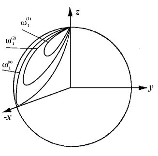
Figure 2: The family of hodographs of vector ${\bf r}={\bf m}/|m_{0}|$ in the conditions of resonance on the shifted frequency $\Delta-\omega_{p}=0$. With the growth of $\omega_{1}(\omega_{1}^{(1)}<\omega_{1}^{(2)}<\ldots\omega_{1}^{(n)})$ the hodographs increase in dimensions and in the limit $\omega_{1}\approx\omega_{p}$ reach the point (-1,00).

3 Analysis of Results of Computer Modeling

For analysis of the above mentioned discussions and investigation of the influence of perturbation on motion of nuclear magnetization the initial equations (1) describing spin-system dynamics were modeled. Modeling was made in the medium of Simulink of mathematical package MATLAB. During the modeling we used stroboscopic method, according to which observation of vector motion of magnetization was conducted not continuously, but during separate, short periodically following one another time intervals.

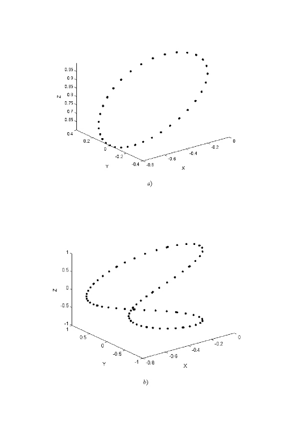
Figure 3: Stroboscopic points of hodographs, which are far from separatrix $(\omega_{1}\neq\omega_{p}).~{}a)~{}\omega_{1}=800Hz,~{}\omega_{p}=1000Hz,~{}\nu_{1}=0;~{}~{}b)~{}\omega_{1}=1000Hz,~{}\omega_{p}=800Hz,~{}\nu_{1}=0$. In both cases the set of stroboscopic points is located periodically.

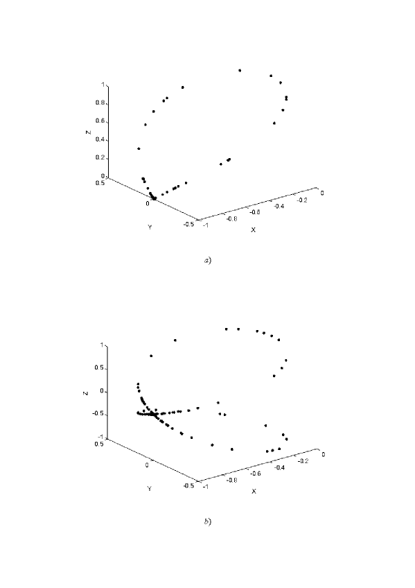
Figure 4: Stroboscopic points of separatrix hodograph: a) $\omega_{1}=\omega_{p}=1000Hz,~{}\nu_{1}=0$. Chaotic points located on the upper part of hodograph. b) $\omega_{1}=\omega_{p}=1000Hz,~{}\nu_{1}=10^{-4}Hz$. Chaotic points located along the whole separatrix hodograph.

Fig.3 shows hodographs distant from separatrix $(\omega_{1}\neq\omega_{p})$. The points being set using stroboscopic method are periodically located along the hodograph. Approaching the separatrix $(\omega_{1}\rightarrow\omega_{p})$ they become chaotic (Fig.4). In the case of $\omega_{1}\approx\omega_{p}$ and $\nu_{1}=0$ chaotic points cover only the upper part of separatrix eight, but after switching on perturbation ($\nu_{1}=10^{-4}Hz$) the motion acts along the whole separatrix one. Stroboscopic points of hodograph are chaotic in this case too. Consequently, a role of slowly changing perturbation is reduced to regular variation of the place of the point of self-crossing separatrix eight.

Thus, stochastic set of points origins close to the singular point (-1,0,0), overcoming of which the motion becomes unpredictable: all four directions, crossing the special point become equally probable. Notice that set of points turned out to be stochastic though external influence on the system is periodical.

As a result of numerical integration of (3) for $z(t)$ at the motion close to the separatrix the solution in the form of periodical succession of instantons is obtained (Fig.5). In the case of $\omega_{1}-\omega_{p}\rightarrow-0$ all the instantons are positive, while at $\omega_{1}-\omega_{p}\rightarrow+0$ in the periodical succession alternate change of instanton sign takes place.

The same result can be obtained also by means of direct set of figures of elliptical functions of Jacob (7).

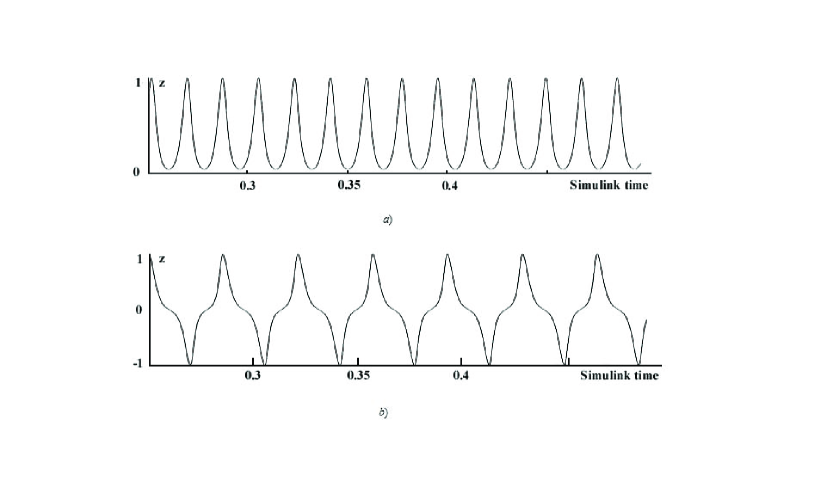
Figure 5: Change of $z$ component of nuclear magnetization during simulation for separatrix close to trajectory $a)~{}\omega_{p}\geq\omega_{1}~{}(\omega_{1}=1000Hz,~{}\omega_{p}=1001Hz,~{}\nu_{1}=0);~{}~{}b)~{}\omega_{p}\leq\omega_{1}~{}(\omega_{1}=1001Hz,~{}\omega_{p}=1000Hz,~{}\nu_{1}=0)$.

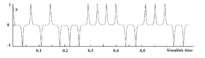
Figure 6: Change of $z$ component of vector of nuclear magnetization during simulation for separatrix trajectory $(\omega_{p}=\omega_{1}=1000Hz,~{}\nu_{1}=10^{-4}Hz)$.

Fig.6 shows the fragment of the picture of changing the sign of $m_{z}$ during simulation already at the switched periodical perturbation ($\nu_{1}=10^{-4}Hz$). Disordered change of the sign of nuclear magnetization testifies an origin of stochasticity at the junction over branching point.

Thus, hodograph of vector of nuclear magnetization at nonlinear NMR on the unshifted frequency in the conditions $\omega_{1}\approx\omega_{p}$ possess the properties of separatrix. This is the basis for appearance of the set of chaotic points in the stroboscopic picture of separatrix hodograph (Fig.3), and also for chaotic change of instantons signs of $z$ component of magnetization (Fig.6).

Acknowledgement

The designated project has been fulfilled by financial support from the Georgian National Foundation (grants: GNSF/STO 7/4-197, GNSF/STO 7/4-179). The financial support of Deutsche Forschungsgemeinschaft through SPP 1285 (contract number EC94/5-1) is gratefully acknowledged by L. Chotorlishvili.

References

- [1] E.A.Turov and M.P.Petrov. Appl. Spectroscopy Rev.,5, 265 (1971).
- [2] S.T. Chui. Phys.Rev., B 55, 3688(1997).
- [3] X. Waintal and O. Parcollet. Phys.Rev. Lett., 94, 247206 (2005).
- [4] D. Xiao, M. Tsoi and Q. Niu. J. Appl. Phys., 99, 013903 (2006).
- [5] W. van Saarloos. Phys. Rep., 386, 29 (2003).
- [6] B.N. Filippov. Low Temp. Phys., 28, 991 (2002).
- [7] G. Bertotti, A. Magni, I.D. Mayergoyz and C. Serpico. J. Appl. Phys., 91, 7559 (2002).
- [8] E.A. Turov and V.V. Nikolaev. Physics Uspekhi, 48, 431 (2005).
- [9] A.I. Ugulava, L.L. Chotorlishvili and Z.Z. Toklikishvili. Low Temp. Phys, 34, 418 (2008).
- [10] D.I. Sementsov and A.M. Shutyi. Physics Uspekhi, 50, 793 (2007).
- [11] A.J. Lichtenberg and M.A. Lieberman. Regular and Stochastic Motion, Springer-Verlag. New York (1983).
- [12] G.M. Zaslavsky. Hamiltonian Chaos and Fractional Dynamics. Oxford University Press. Oxford (2005).
- [13] H. Mabuchi and A. Doherty. Science., 298, 1372 (2002).
- [14] C.J. Hood, T.W. Lynn, A.C. Doherty, A.S. Parkins and H.J.Kimble. Science., 287, 1447 (2000).
- [15] J. Raimond, M. Brune, S. Haroche. Rev. Mod. Phys., 73, 565 (2001).
- [16] L. Chotorlishvili and Z. Toklikishvili. Phys. Lett. A, 372, 2806 (2008).
- [17] L. Chotorlishvili, Z. Toklikishvili and J. Berakdar. Phys. Lett. A, 373, 231 (2009).
- [18] E.A. Turov, M.I. Kurkin and V.V. Nikolaev. JETP, 64, 283 (1973).
- [19] M.P. Strzys, E.M. Graefe and H.J. Korsch. New Journal of Physics, 10, 1 (2008).
- [20] A.I. Ugulava. Low Temp. Phys, 3, 227 (1987).