The Evolutionary History of Lyman Break Galaxies Between Redshift 4 and 6: Observing Successive Generations of Massive Galaxies in Formation

Abstract

We present new measurements of the evolution in the Lyman break galaxy (LBG) population between $z\simeq 4$ and $z\simeq 6$. By utilizing the extensive multiwavelength datasets available in the GOODS fields, we identify 2443 B, 506 V, and 137 $i^{\prime}$-band dropout galaxies likely to be at $z\approx 4$, $5$, & $6$. For the subset of dropouts for which reliable Spitzer IRAC photometry is feasible (roughly 35% of the sample), we estimate luminosity-weighted ages and stellar masses. With the goal of understanding the duration of typical star formation episodes in galaxies at $z\mathrel{\hbox to0.0pt{\lower 4.0pt\hbox{\hskip 1.0pt$\sim$}\hss}\raise 1.0pt\hbox{$>$}}4$, we examine the distribution of stellar masses and ages as a function of cosmic time. We find that at a fixed rest-UV luminosity, the average stellar masses and ages of galaxies do not increase significantly between $z\simeq 6$ and 4. In order to maintain this near equilibrium in the average properties of high redshift LBGs, we argue that there must be a steady flux of young, newly-luminous objects at each successive redshift. When considered along with the short duty cycles inferred from clustering measurements, these results may suggest that galaxies are undergoing star formation episodes lasting only several hundred million years. In contrast to the unchanging relationship between the average stellar mass and rest-UV luminosity, we find that the number density of massive galaxies increases considerably with time over $4\mathrel{\hbox to0.0pt{\lower 4.0pt\hbox{\hskip 1.0pt$\sim$}\hss}\raise 1.0pt\hbox{$<$}}z\mathrel{\hbox to0.0pt{\lower 4.0pt\hbox{\hskip 1.0pt$\sim$}\hss}\raise 1.0pt\hbox{$<$}}6$. Given this rapid increase of UV luminous massive galaxies, we explore the possibility that a significant fraction of massive (10¹¹ M_⊙) $z\simeq 2-3$ distant red galaxies (DRGs) were in part assembled in an LBG phase at earlier times. Integrating the growth in the stellar mass function of actively forming LBGs over $4\mathrel{\hbox to0.0pt{\lower 4.0pt\hbox{\hskip 1.0pt$\sim$}\hss}\raise 1.0pt\hbox{$<$}}z\mathrel{\hbox to0.0pt{\lower 4.0pt\hbox{\hskip 1.0pt$\sim$}\hss}\raise 1.0pt\hbox{$<$}}6$ down to $z\simeq 2$, we find that $z\mathrel{\hbox to0.0pt{\lower 4.0pt\hbox{\hskip 1.0pt$\sim$}\hss}\raise 1.0pt\hbox{$>$}}3$ LBGs could have contributed significantly to the quiescent DRG population, indicating that the intense star-forming systems probed by sub-millimeter observations are not the only route toward the assembly of DRGs at $z\simeq 2$.

1. Introduction

The detailed study of various classes of distant galaxies has enabled great progress in understanding the star formation and mass assembly history of normal field galaxies (for recent reviews see Hopkins & Beacom 2006; Ellis 2008; Wilkins et al. 2008). Multi-wavelength probes have been particularly effective in revealing the co-existence of diverse categories of galaxies with redshifts $z\simeq 2$-3. These include the relatively unobscured star-forming ‘Lyman break’ galaxies (LBGs, e.g., Steidel et al. 1996; Shapley et al. 2005), the infrared-selected massive ‘distant red’ galaxies (DRGs, e.g., Franx et al. 2003; van Dokkum et al. 2006) and heavily obscured sub-mm galaxies which contain both intensely star-forming and active components (SMGs, e.g. Smail et al. 1998; Chapman et al. 2005). The collective study of these populations has revealed that the redshift range $1<z<3$ is a formative one when the bulk of the stars in present-day massive galaxies was produced (Hopkins & Beacom, 2006).

Understanding the inter-relationship between these various sources is an important goal and intense efforts are now underway to address this issue (e.g., van Dokkum et al. 2006; Reddy et al. 2008). A relevant aspect of this discussion concerns the assembly history of objects observed during the redshift interval $4<z<6$, corresponding to a period only 1 Gyr earlier. Such data may provide valuable insight into the connection between actively star-forming and passive populations as well as define the mode of star formation in typical massive galaxies.

Over the last five years, deep multiwavelength surveys have resulted in the discovery of large samples of LBGs at $z\simeq 4-6$ (Bouwens et al., 2007). Despite early controversies (Bunker et al., 2004; Stanway et al., 2003; Giavalisco et al., 2004a; Beckwith et al., 2006), it now seems clear that the star formation density declines with redshift beyond $z\simeq 3$. Recent evidence also suggests the characteristic luminosity is also fading (Yoshida et al., 2006; Bouwens et al., 2007; McLure et al., 2008). Bouwens et al. (2007) attribute this evolutionary pattern to the simple hierarchical assembly of galaxies. Unfortunately, because of the transient nature of star formation probed by the rest-frame UV luminosity function, these studies alone provide only an approximate measure of the evolutionary processes occurring during $3<z<6$. Key to testing the mode of assembly of galaxies in this early period is additional information on the physical properties, such as the associated stellar mass and the inferred age of the stellar populations. The availability of deep IRAC data for many of the HST fields enables such an approach (Egami et al., 2005; Eyles et al., 2005; Yan et al., 2005).

In this paper, we aim to improve our understanding of galaxy evolution during the first 2 Gyr by systematically tracking the evolving stellar content of star-forming galaxies in uniformly-selected samples spanning three separate redshift intervals between $z\simeq 4$ and 6. By adding the additional physical parameters of stellar mass and luminosity-weighted ages, we can break degeneracies associated with studies that rely only on the UV luminosity function.

An important issue is how and when the quiescent subset of DRGs seen at $z\simeq 2-3$ (van Dokkum et al., 2006; Kriek et al., 2006) assembled their mass. Contemporary models of galaxy formation suggest that the number density of massive galaxies increases continuously with cosmic time over $2\mathrel{\hbox to0.0pt{\lower 4.0pt\hbox{\hskip 1.0pt$\sim$}\hss}\raise 1.0pt\hbox{$<$}}z\mathrel{\hbox to0.0pt{\lower 4.0pt\hbox{\hskip 1.0pt$\sim$}\hss}\raise 1.0pt\hbox{$<$}}5$ (Bower et al., 2006), a picture supported by the relatively young ages of massive DRGs at $z\simeq 2$ (Kriek et al., 2006). Alternatively, it is potentially feasible that the bulk of the most massive systems at $z\simeq 2$ formed their mass at much earlier times (e.g., $z\mathrel{\hbox to0.0pt{\lower 4.0pt\hbox{\hskip 1.0pt$\sim$}\hss}\raise 1.0pt\hbox{$>$}}5$) which in turn would imply little evolution in the number density of massive galaxies over 3$\mathrel{\hbox to0.0pt{\lower 4.0pt\hbox{\hskip 1.0pt$\sim$}\hss}\raise 1.0pt\hbox{$<$}}z\mathrel{\hbox to0.0pt{\lower 4.0pt\hbox{\hskip 1.0pt$\sim$}\hss}\raise 1.0pt\hbox{$<$}}6$. We seek to constrain the formation epoch of quiescent DRGs by studying the evolving stellar mass function of star-forming galaxies over $4\mathrel{\hbox to0.0pt{\lower 4.0pt\hbox{\hskip 1.0pt$\sim$}\hss}\raise 1.0pt\hbox{$<$}}z\mathrel{\hbox to0.0pt{\lower 4.0pt\hbox{\hskip 1.0pt$\sim$}\hss}\raise 1.0pt\hbox{$<$}}6$. Moreover, we wish to understand whether most DRGs were assembled entirely in intense, dust-enshrouded star formation episodes (probed by higher redshift SMGs), or if a significant fraction were formed in less vigorous star-forming systems traced by higher redshift LBGs. By determining the number density of massive galaxies in the LBG phase at each redshift interval, we hope to estimate the fraction of DRGs whose progenitors formed a significant component of their mass in relatively unobscured systems with moderate star formation rates (SFR) typical of the LBG population (e.g., Shapley et al. 2001, 2005).

A further question of significance in characterizing the mode of early galaxy assembly is understanding the duration of star formation episodes in high redshift galaxies. In the context of models in which gas accretion dominates galaxy growth at high redshift (e.g., Birnboim & Dekel 2003; Kereš et al. 2005; Finlator et al. 2007) leading to rapid and steady star formation, one might imagine that the LBGs seen at $z\simeq 4$ have evolved relatively smoothly since their formation at an earlier epoch, creating stars at a near constant rate. If their assembly timescales are long enough, we would thus expect similarly luminous $z\simeq 5$ and 6 LBGs to be less evolved versions than their $z\simeq 4$ descendants with lower stellar masses and younger ages. Alternatively, it is conceivable that this era witnesses a rapid increase in the intensity of star formation in individual galaxies, as has been predicted for the early stages of galaxy growth (Kereš et al., 2005; Finlator et al., 2007). In this case, galaxies would grow along a locus of points (or “main sequence”) in the $\rm{M_{\star}}$-SFR plane. Thus, if viewed at fixed UV luminosity, the observed stellar populations would not vary significantly from one redshift to another. Finally, in contrast to these “sustained” star formation histories, we may expect star formation episodes to occur on much shorter timescales. If the past duration of star formation is sufficiently short ($\mathrel{\hbox to0.0pt{\lower 4.0pt\hbox{\hskip 1.0pt$\sim$}\hss}\raise 1.0pt\hbox{$<$}}300$ Myr), then each dropout sample would be dominated by newly emerged systems, and we would not necessarily expect to see significant growth in the $\rm{M_{\star}}$-SFR plane over the redshift range studied.

Earlier work in this direction has been promising but the datasets have been limited. Drory et al. (2005) traced the mass assembly of galaxies to high redshift using K-band selected samples. However since their study did not include IRAC data, reliable stellar masses could only be derived to $z\simeq 4.5$. Verma et al. (2007) used HST and IRAC data to compare the stellar mass and age distribution of a small, robust sample of $z\simeq 5$ LBGs to those derived by Shapley et al. (2001) at $z\simeq 3$. Most recently, McLure et al. (2008) computed the stellar mass function of LBGs at $z\simeq 5$ and 6 by scaling the UV luminosity function by the average mass/light ratio of the LBG population at high redshift. While these efforts have improved our understanding of the stellar content of high-redshift galaxies, none has yet systematically traced the evolving stellar populations of galaxies over the full redshift range, using large and uniformly selected samples with no scaling assumptions.

A plan of the paper follows. In §2, we describe the GOODS data used in our analysis. In §3, we discuss the color selection used to identify dropouts, and criteria used to remove contaminants from our sample. We close the section by assessing the evolving surface densities of the dropouts. In §4, we consider the mid-infrared properties of the dropouts and in §5, we discuss the population synthesis models used to infer stellar masses and ages and comment on the uncertainties in the derived properties. In §6, we examine the redshift evolution in the stellar masses and ages of dropouts at a fixed UV luminosity. Using this information, we discuss the implications for the star formation histories of galaxies at high redshift. In §7, we study the evolving stellar mass functions of LBGs over $4\mathrel{\hbox to0.0pt{\lower 4.0pt\hbox{\hskip 1.0pt$\sim$}\hss}\raise 1.0pt\hbox{$<$}}z\mathrel{\hbox to0.0pt{\lower 4.0pt\hbox{\hskip 1.0pt$\sim$}\hss}\raise 1.0pt\hbox{$<$}}6$ and estimate the fraction of LBGs that evolve into quiescent massive galaxies at $z\simeq 2-3$. Finally in §8, we compute the stellar mass densities of the B, V, and $i^{\prime}$-drop samples.

Throughout the paper, we adopt a $\Lambda$-dominated, flat universe with $\Omega_{\Lambda}=0.7$, $\Omega_{M}=0.3$ and $\rm{H_{0}}=70\,\rm{h_{70}}{\rm km\,s}^{-1}\,{\rm Mpc}^{-1}$. All magnitudes in this paper are quoted in the AB system (Oke & Gunn, 1983).

2. Data

2.1. The GOODS Fields

We focus our analysis on the data from the Great Observatories Origins Deep Survey (GOODS). Detailed descriptions of the datasets are available in the literature (Giavalisco et al., 2004b), so we only provide a brief summary here. The GOODS-S and GOODS-N survey areas each cover roughly 160 arcmin² and are centered on the Chandra Deep Field South (CDF-S; Giacconi et al. 2002) and the Hubble Deep Field North (HDF-N; Williams et al. 1996). Extensive multiwavelength observations have been conducted in each of these fields. In this paper, we utilize optical imaging from the Advanced Camera for Surveys (ACS) onboard the Hubble Space Telescope (HST). Observations with ACS were conducted in F435W, F606W, F775W, and F850LP (hereafter B₄₃₅, V₆₀₆, $i^{\prime}_{775}$, $z^{\prime}_{850}$) toward GOODS-S and GOODS-N (Giavalisco et al., 2004b). The average 5$\sigma$ limiting magnitudes in the v1 GOODS ACS data (correcting for the flux that lies outside the 0$\farcs$5 diameter photometric aperture) are B₄₃₅=27.8, V₆₀₆=28.0, $i^{\prime}_{775}$=27.2, and $z^{\prime}_{850}$=27.0. We also make use of U-band observations of GOODS-N taken with the Kitt Peak National Observatory 4-m telescope with the MOSAIC prime focus camera (Capak et al., 2004) and of GOODS-S taken with the Wide-Field Imager mounted on the 2.2m MPG/ESO telescope (Arnouts et al., 2001).

In the near-infrared, we utilize publicly available deep J and K-band observations of GOODS-S (PI: C. Cesarsky) using the ISAAC camera on the Very Large Telescope (VLT). The sensitivities vary across the field depending on the effective integration time and seeing FWHM. Average 5$\sigma$ magnitude limits (corrected for the amount of flux that falls outside of the 1$\farcs$0 diameter aperture) are $J\simeq 25.1$ and K${}_{s}\simeq 24.6$. Toward GOODS-N, we make use of a new Subaru K-band mosaic of the field (Bundy et al., 2009) using the MOIRCS camera (Ichikawa et al., 2006). The specifics of the observations are described in detail in Bundy et al. (2009). The 5$\sigma$ limiting magnitude varies between $K_{s}=23.9$ and 24.1 (after aperture correction) across the mosaic.

Deep Spitzer imaging is available toward both GOODS fields with the Infrared Array Camera (IRAC) as part of the “Super Deep” Legacy program (Dickinson et al. in prep, Chary et al. in prep). Details of the observations have been described in detail elsewhere (Eyles et al., 2005; Yan et al., 2005; Stark et al., 2007) so we do not discuss them further here. The 5$\sigma$ limiting magnitudes of the IRAC imaging are $\simeq 25.9$ at 3.6$\mu$m and $\simeq 25.5$ at 4.5$\mu$m using 2$\farcs$4 diameter apertures and applying an aperture correction (see §2.3).

In a later section (§3.3), we will revisit the sensitivity limits of the GOODS datasets, utilizing completeness simulations to determine magnitude limits for our survey.

2.2. Optical Photometry

ACS photometry was obtained from the GOODS team r1.1 catalog  which ws generated from the v1 GOODS ACS reduction. The photometric zeropoints adopted in the catalog are 25.653, 26.493, 25.641, and 24.843 for the $B_{435}$-band, $v_{606}$-band, $i^{\prime}_{775}$ band, and $z^{\prime}_{850}$-band, respectively. We have corrected for the small amount of foreground Galactic extinction using the COBE/DIRBE & IRAS/ISSA dust maps of Schlegel et al. (1998); for the GOODS-S field, the color excess is given by E($B-V$) = 0.008 mag; in GOODS-N, the color excess is given by E($B-V$) = 0.012 mag. Colors are computed using magnitudes measured 0$\farcs$50-diameter apertures. As detailed further in §3.1, total magnitudes are computed using a combination of the aperture colors and MAG_AUTO SExtractor parameter.

2.3. Near- and mid-infared Photometry

Near-infrared fluxes were computed on each of the sources in the GOODS r1.1 catalog. We utilized $1^{\prime\prime}$-diameter apertures centered on the source positions in the ACS images. The seeing varied across the GOODS-S and GOODS-N fields as different tiles were taken over many nights, so we determined separate aperture corrections from unresolved sources for each tile. For the $J$ and $K_{s}$-band ISAAC images the seeing is typically good (${\rm FWHM}=0\farcs 4-0\farcs 5$), and the aperture corrections are $\approx 0.3-0.5$ mag, determined from bright but unsaturated isolated stars measured in $6^{\prime\prime}$-diameter apertures. Likewise, the MOIRCS GOODS-N $K_{s}$-band seeing was fairly constant at FWHM=0$\farcs$5; photometry was again computed in $1^{\prime\prime}$-diameter apertures and the aperture corrections are typically 0.3-0.7 mag.

For the GOODS IRAC images, magnitudes are measured in relatively small apertures ($\approx 1.5\times{\rm FWHM}$ which corresponds to a diameter of 2$\farcs$4) to maximize the signal-to-noise ratio ($S/N$). We applied aperture corrections to compensate for the flux falling outside the aperture: these were $\approx 0.7$ mag for the IRAC 3.6 and 4.5 $\mu$m data, as determined from bright but unsaturated point sources in the images using large apertures. The PSF of IRAC leads to frequent blending with nearby sources, so care must be taken to ensure that the photometry is robust. We discuss our strategy for dealing with this in §4.

3. Selection of High-Redshift Galaxies

The goal of this section is to compile a robust sample of dropouts at $z\simeq 4$, 5, and 6. In §3.1, we identify B, V, and $i^{\prime}$-dropouts using standard selection criteria (e.g., Giavalisco et al. 2004a; Beckwith et al. 2006; Bouwens et al. 2007). We excise low-redshift and stellar contaminants from these samples using a combination of photometric, spectroscopic, and morphological techniques (§3.2). In §3.3, we compute the completeness limits of our data and determine the surface density of our samples.

3.1. Dropout Selection

Galaxies at $z\simeq 4$, 5, and 6 are selected via the presence of the Lyman-break as it is redshifted through the B₄₃₅, V₆₀₆, and $i^{\prime}_{775}$ bandpasses, respectively. Selection of Lyman break galaxies at these redshifts has now become routine (Stanway et al., 2003; Giavalisco et al., 2004a; Bunker et al., 2004; Beckwith et al., 2006; Bouwens et al., 2007). In order to ensure a consistent comparison of our samples to these previous samples, we adopt color criteria which are identical to those used in Beckwith et al. (2006) and very similar to those used by Bouwens et al. (2007). These criteria have been developed to select galaxies in the chosen redshift interval while minimizing contamination from red galaxies likely to be at low redshift. We detail our color-selection and S/N limit criteria for selecting dropouts below.

As mentioned in the previous section, galaxies are selected from the GOODS version r1.1 ACS multi-band source catalogs. In these catalogs, source detection has been performed using the $z^{\prime}_{850}$-band images.

Conditions for selection as B₄₃₅-drop :

$$B_{435}-V_{606} > (1.1+V_{606}-z^{\prime}_{850})$$ (1)

$$B_{435}-V_{606} > 1.1$$ (2)

$$V_{606}-z^{\prime}_{850} < 1.6$$ (3)

$$S/N(V_{606}) > 5$$ (4)

$$S/N(i^{\prime}_{775}) > 3$$ (5)

In addition we also examine each B-drop for a detection in the U-band images described in the previous section. B-band dropouts at $z\mathrel{\hbox to0.0pt{\lower 4.0pt\hbox{\hskip 1.0pt$\sim$}\hss}\raise 1.0pt\hbox{$>$}}3.5$ should not show strong detections in the U-band as it lies shortward of the dropout filter. We look at each source with a U-band detection (2$\sigma$ or more) to make sure that the flux is not spurious or associated with another object. In total, we excise four sources based on the presence of U-band flux.

Conditions for selection as V₆₀₆-drop:

$$V_{606}-i^{\prime}_{775} > 1.47+0.89(i^{\prime}_{775}-z^{\prime}_{850})$$ (6)

$${\rm or}\ \ 2$$

$$V_{606}-i^{\prime}_{775} > 1.2$$ (7)

$$i^{\prime}_{775}-z^{\prime}_{850} < 1.3$$ (8)

$$S/N(z^{\prime}_{850}) > 5$$ (9)

$$S/N(B_{435}) < 2\hskip 28.45274pt{\rm or}\ \$$

$$B_{435}-i_{775} > V_{606}-i^{\prime}_{775}+1$$ (10)

Conditions for selection as $i^{\prime}_{775}$-drop:

$$i^{\prime}_{775}-z^{\prime}_{850} > 1.3$$ (11)

$$S/N(z^{\prime}_{850}) > 5$$ (12)

$$S/N(V_{606}) < 2\hskip 28.45274pt{\rm or}\ \$$

$$V_{606}-z^{\prime}_{850} > 2.8$$ (13)

In order to utilize these dropout criteria, we must compute accurate colors and total magnitudes for each source in the GOODS catalogs. The colors are computed using the aperture magnitudes discussed in §2.2. We adopt the $i^{\prime}_{775}$-band MAG_AUTO magnitude as the total $i^{\prime}_{775}$-band magnitude for the B₄₃₅-drops. Total magnitudes are subsequently computed in the B₄₃₅, V₆₀₆, and $z^{\prime}_{850}$-bands using the B${}_{435}-i^{\prime}_{775}$, V${}_{606}-i^{\prime}_{775}$, $i^{\prime}_{775}-z^{\prime}_{850}$ colors measured using aperture magnitudes (0$\farcs$50-diameter). Similarly, total magnitudes are computed for the V₆₀₆ and $i^{\prime}_{775}$-drops taking the $z_{850}$-band MAG_AUTO magnitude and B${}_{435}-z^{\prime}_{850}$, V${}_{606}-z^{\prime}_{850}$, $i^{\prime}_{775}-z^{\prime}_{850}$ colors. The S/N limits stated above are determined from the measured flux and error in the total magnitudes and vary depending on the noise background at the location of the source. On average, these limits are well represented by the magnitudes presented in §2.2.

Figure 1.— Histogram of $i^{\prime}_{775}$ and $z^{\prime}_{850}$ magnitudes for 2819 B-drops, 615 V-drops, and 166 $i^{\prime}$-drops in GOODS-S and GOODS-N. In each panel, the open histogram corresponds to the total sample of dropouts while the filled histogram corresponds to only those sources that are isolated in Spitzer (see §4.1).

We examine each source in the dropout catalogs, removing diffraction spikes from bright stars, image artifacts, and spurious features (primarily along the edges of the GOODS mosaic), leaving a sample of 2819 B-drops, 615 V-drops, and 166 $i^{\prime}$-drops. A histogram of the measured optical magnitudes for the three dropout samples is presented in Figure 1. In the next section, we seek to further refine these samples, identifying and removing stellar and low-redshift interlopers.

3.2. Removal of Stellar and Low-z Contaminants

The Lyman-break selection is well known to include a variety of interlopers in addition to the desired high-redshift galaxies. Standard contaminants include cool stars and dusty or old galaxies at lower-redshifts (e.g., Stanway et al. 2004; Beckwith et al. 2006; Bouwens et al. 2006). We first seek to morphologically identify and excise stellar interlopers from the dropout catalogs. To assess the fraction of dropouts at low redshift, we first mine the existing spectroscopic surveys for known redshifts of our sample. We then proceed to compute photometric redshifts for all the remaining dropouts without spectroscopic redshifts and compute the uncertainty in the photometric redshifts.

We identify stellar contaminants by their morphology, removing all bright ($z^{\prime}_{850}<26.0$) sources with SExtractor stellarity parameter greater than 0.80. We found that this value (very similar to those used in Bouwens et al.) was optimal in distinguishing between spectroscopically confirmed galaxies and stars. Applying this criteria removes 51 B-drops (20 in GOODS-S, 31 in GOODS-N), 23 V-drops (12 in GOODS-S, 11 in GOODS-N), and 8 $i^{\prime}$-drops (3 in GOODS-S, 5 in GOODS-N) from our sample. Faintward of this limit, the S/N of the GOODS data is too low to reliably identify stars by their stellarity index. Following the approach taken in Bouwens et al. (2006), we estimate the number of faint stellar contaminants that remain in the GOODS dropout catalog by examining dropout samples in the Hubble Ultra Deep Field (HUDF); the exquisite data quality of the HUDF enables point sources to be identified with sufficient S/N for sources that would be located at the sensitivity limits of the GOODS data. Using the same dropout criteria as in GOODS, we select B, V, and $i^{\prime}$-drops in the HUDF using publicly-available $z_{850}$-band source catalogs (Coe et al., 2006). We find that the fraction of dropouts with stellarity indices above 0.8 over the magnitude interval $26<z_{850}<28$ is very low for the B-drops (0/171), V-drops (0/35), and $i^{\prime}$-drops (0/21). These results support the findings of previous studies (e.g. Bunker et al. 2004; Pirzkal et al. 2005; Bouwens et al. 2006, 2007) that stellar contaminants are most prevalent at relatively bright magnitudes (e.g., $z_{850}<26$).

Dropouts in the GOODS fields have been observed spectroscopically with VLT/FORS2 (Vanzella et al., 2002, 2005, 2008, 2009), Gemini/GMOS Nod& Shuffle (Stanway et al., 2004, 2007) , and Keck/DEIMOS (Stanway et al., 2004). The results of the VLT/FORS2 survey are made public in a large database of 1165 total spectroscopic redshifts in GOODS-S (Vanzella et al., 2008). We search the database (version 3.0) for each of the dropouts using an 0.5-arcsecond matching diameter. Thirty-seven B-drops have spectroscopic redshifts ranging between $z$=3.19 and 4.73 with a median redshift of 3.7. We remove the one B-drop with a low-redshift ($z$=1.54) identification from our sample. Twenty-four V-drops have spectroscopic redshifts at $z>4$ with a median redshift of 4.81. Finally, 20 $i^{\prime}$-drops have spectroscopic redshifts at $z>5$, while one $i^{\prime}$-drop (which we subsequently remove) has a low-z identification ($z$=1.32).

Photometric redshifts and their associated probabilities have been determined for each remaining dropout by fitting the observed SEDs against template galaxy SEDs of various ages, spectral types, and redshifts using the Bayesian Photometric Redshift (BPZ) software (Benítez, 2000). We fit the observed optical through near-IR SED against templates from Coleman et al. (1980) and the starburst templates from Kinney et al. (1996) and a very young (10 Myr) starburst template derived from the Charlot & Bruzual 2007 (hereafter CB07) models assuming an exponentially decaying star formation history with $\tau$=100 Myr, no dust, and a metallicity of 0.2 Z_⊙. The code outputs both a Bayesian and maximum-likelihood photometric redshift (and associated probability).

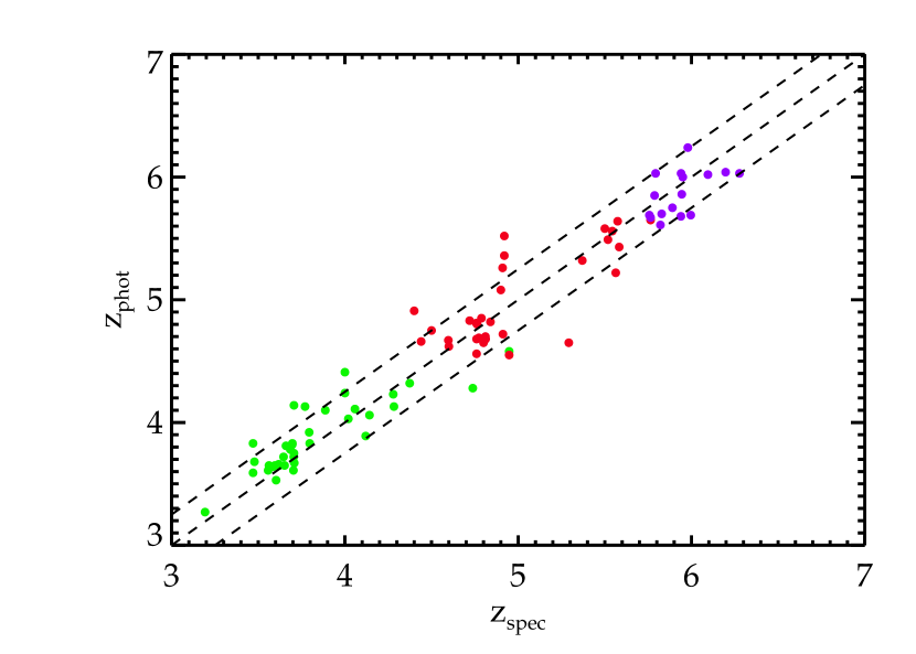
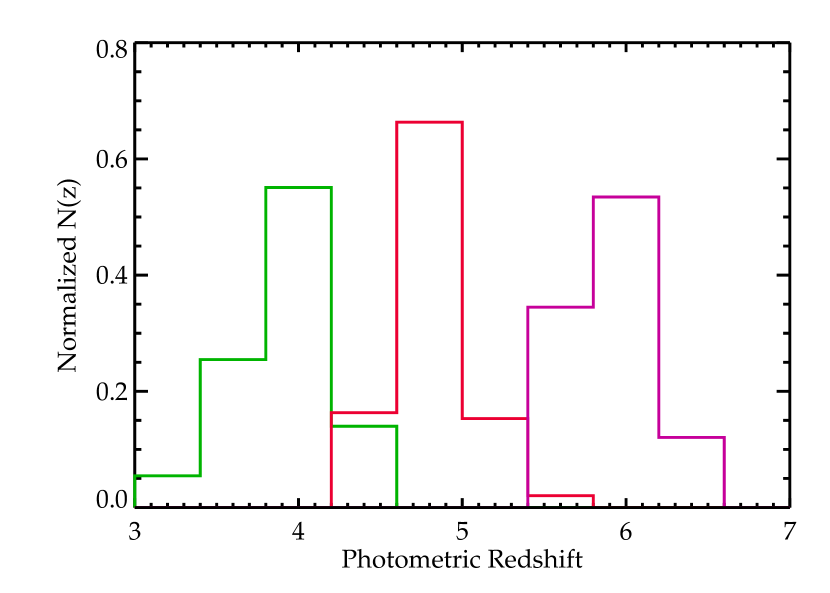
Figure 2.— Top: Comparison of photometric and spectroscopic redshifts for dropouts with redshifts measured with FORS2 from (Vanzella et al., 2008). The center dashed line denotes the unity relationship, while the two additional dashed lines correspond to $\Delta$z=z_spec-z_phot=0.25. Bottom: Distribution of photometric redshifts in B, V, and $i^{\prime}$-drop IRAC-clean samples, normalized to the total sample size. The median inferred redshift is 3.96, 4.75, and 6.01 for the B, V, and $i^{\prime}$-drop samples, respectively.

In Figure 2a, we present the derived maximum-likelihood photometric redshifts for the sample of dropouts with known spectroscopic redshifts from FORS2. The root mean square (RMS) difference between the photometric and spectroscopic estimates is 0.19, 0.25, and 0.18 for the B-drops, V-drops, and $i^{\prime}$-drops, respectively, excluding one spectroscopically-confirmed source with an anomalously low photometric redshift. We find that the RMS uncertainty in our BPZ photometric redshifts is similar to that from the GOODS MUSIC catalog (Grazian et al., 2006) for the subset of dropouts with spectroscopic redshifts.

We next attempt to eliminate lower redshift contaminants which made their way through the initial color cut, removing those sources with photometric redshifts that lie below z${}_{\rm{phot}}<3$, $4$, $5$ in the B, V, and $i^{\prime}$-drops. In order to avoid removing viable high-redshift sources, we only remove those sources whose summed redshift probability distribution suggests that they are very likely ($\mathrel{\hbox to0.0pt{\lower 4.0pt\hbox{\hskip 1.0pt$\sim$}\hss}\raise 1.0pt\hbox{$>$}}70$%) to lie at low redshift. Sources with near equal maxima at low and high redshift can not be confidently included or excluded. However these sources are small in number. The inclusion or exclusion of this subset with ambiguous photometric redshifts does not affect the observed optical or infrared magnitude distribution. Following this appraoch, the BPZ photometric redshifts require the removal of 258, 47, and 14 (10, 8, and 9%) of the B, V, and $i^{\prime}$-drop candidates from the catalogs, leaving a sample of 2443, 506, and 137 B, V, and $i^{\prime}$-dropouts across both GOODS fields. In general, the excised sources are either marginally detected in the optical or very red in their $z^{\prime}_{850}-K$ colors, as would be expected for low-redshift sources which satisfy the dropout criteria.

In Figure 2b, we present the distribution of photometric redshifts from the remaining high redshift samples in bins of $\Delta$z=0.4. The median and standard deviation photometric redshifts of the resulting B, V, and $i^{\prime}$-drop samples are $z_{phot}$=3.96$\pm$0.29, 4.79$\pm$0.25, and 6.01$\pm$0.25 respectively. These distributions are in rough agreement with those computed in (Bouwens et al., 2007).

3.3. Surface Densities and Effective Volume

The GOODS datasets allow sources to be selected down to magnitudes fainter than $m_{AB}=27$; however, as is apparent in Figure 1, the completeness begins to decline brightward of this limit. Hence, to compute the correct density of dropouts, we must account for this variation in completeness with apparent magnitude.

To do this, we define a function $p(m,z)$ that represents the probability that a galaxy with apparent magnitude m and redshift $z$ is recovered in our dataset. We compute this function for each of the three dropout samples by putting thousands of fake galaxies into the GOODS images and recreating a photometric catalog for the new image using the selection parameters described above. The apparent magnitudes of the fake galaxies span $i^{\prime}_{775}=21-28$ (B-drops), $z^{\prime}_{850}=22-28$ (V-drops), $z^{\prime}_{850}=23-28$ ($i^{\prime}$-drops) and their redshifts span the interval 3.0$<z<$4.9 for the B-drops, 4.0$\leq z\leq$5.9 for the V-drops, and 5.0$<z<$7.6 for the $i^{\prime}$-drops in steps of $\Delta z$=0.1. The sizes of the fake galaxies are chosen to be consistent with distribution of half-light radii derived for $z\simeq 4-6$ galaxies in Bouwens et al. (2004). The colors of the fake galaxies depend on the galaxy redshift and spectral energy distribution (SED). In order to compute these colors, we use the SED of a CB07 model with constant star formation history, an age of 100 Myr, and no dust as the intrinsic rest-frame SED of the fake galaxies. Allowing for a younger age or a color excess of E(B-V)=0.1 in the fake galaxies’ SEDs alters the completeness by roughly 5%, which would not significantly change any of our results. The colors are computed at each redshift after applying the appropriate IGM absorption (e.g. Madau 1995) to the SED. The probability function, $p(m,z)$ is then given by the fraction of fake galaxies with apparent magnitude, m, and redshift, $z$, that satisfy the dropout color selection criteria defined in §2.4.

We next determine the volume observed as a function of apparent magnitude for each of the dropout samples following the approach of Steidel et al. (1999) using

$$V_{\rm eff}(m)=\int dz\,p(m,z)\,\frac{dV}{dz}$$ (14)

where $p(m,z)$ is the probability of detecting a galaxy at redshift $z$ and apparent magnitude $m$, and $dz\,\frac{dV}{dz}$ is the comoving volume per unit solid angle in a slice $dz$ over the redshift interval 3.0$<z<$4.9 for the B-drops, 4.0$\leq z\leq$5.9 for the V-drops, and 5.0$<z<$7.6 for the $i^{\prime}$-drops.

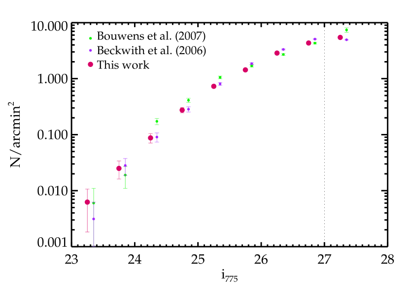
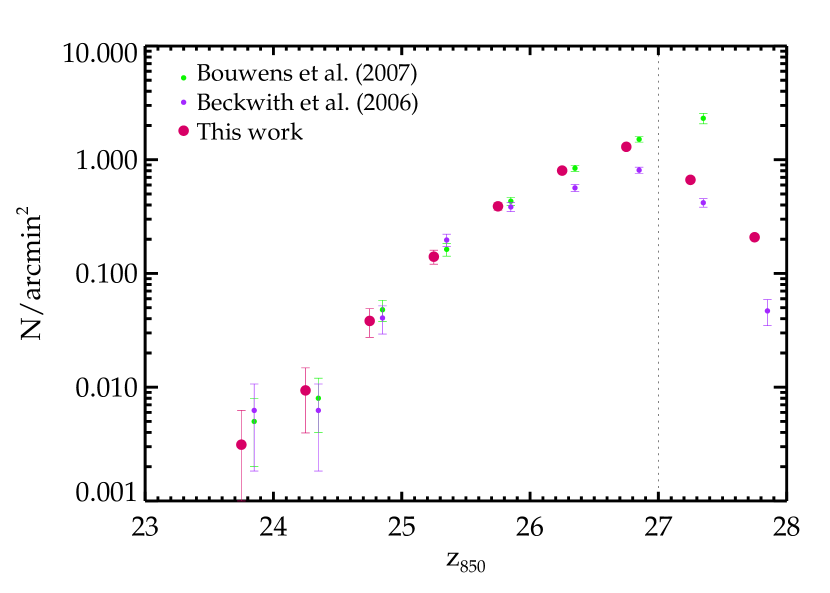
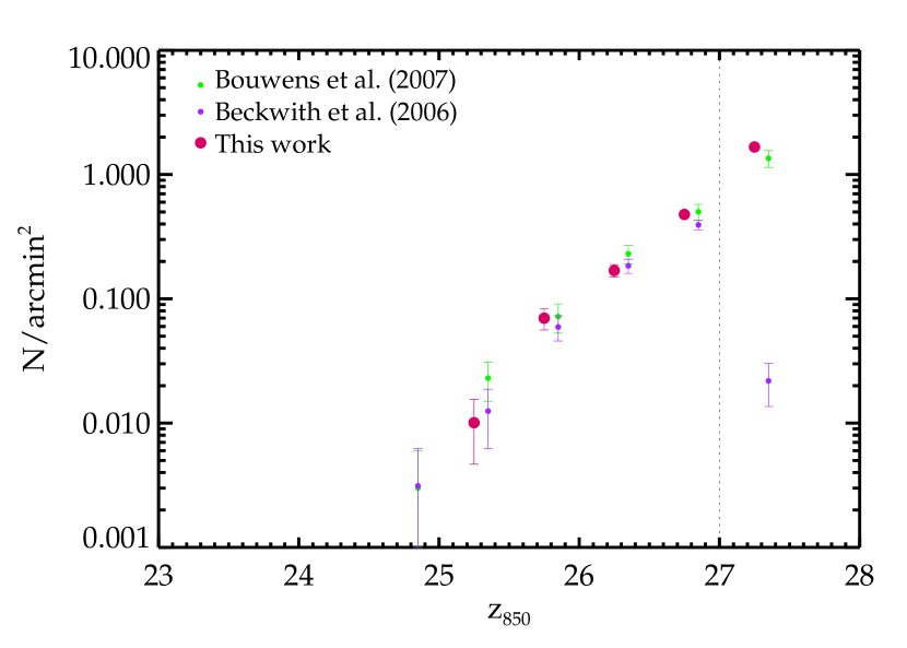
Figure 3.— Surface densities of dropout samples. Stars, artifacts, and low-$z$ galaxies have been removed from the initial sample as described in §3.2. We place the remaining sample in magnitude bins spanning 0.5 mags and adjust the measured densities for incompleteness (§3.3). Our samples are sufficiently complete brightward of 27th magnitude (vertical dotted lines) to enable reliable density measurements. The resulting surface densities are in excellent agreement with previous measurements.

The effective volumes are subsequently computed as a function of apparent magnitude for the dropout samples following equation 14. In general, for the dropout samples in a single GOODS field, the effective volumes drop from 4-$5\times\rm{10}^{5}$ Mpc³ at bright magnitudes ($m_{\rm{AB}}$=23.5) to $2\times\rm{10}^{5}$ Mpc³ at fainter magnitudes ($m_{\rm{AB}}$=27), reflecting $\simeq 50$% completeness, on average, at the limit of our samples. In Figure 3, we show the derived surface densities of our dropouts, corrected using the magnitude-dependent completeness $p(m)$ derived in equation above. The measured values are in excellent agreement (generally to within 1$\sigma$) with previous measurements (Bouwens et al., 2007) at AB magnitudes brighter than 27. Faintward of this limit, the completeness in the GOODS data is too low to enable reliable density measurements.

4. Mid-infrared Properties of Dropouts

4.1. Construction of Spitzer-Isolated Subsample

Mid-infrared photometry is the crucial component for estimating the stellar populations of $z\mathrel{\hbox to0.0pt{\lower 4.0pt\hbox{\hskip 1.0pt$\sim$}\hss}\raise 1.0pt\hbox{$>$}}4$ galaxies. However the low spatial resolution of Spitzer results in frequent blending between nearby sources, making accurate photometry of individual objects difficult. To ensure that objects in our sample were not contaminated by neighboring bright foreground sources, we examined each dropout by eye and flagged sources that are hopelessly confused with flux from bright, nearby sources.

Following Stark et al. (2007), we only apply population synthesis models to those objects which are unconfused in the IRAC images, which we define as having no bright ($\mathrel{\hbox to0.0pt{\lower 4.0pt\hbox{\hskip 1.0pt$\sim$}\hss}\raise 1.0pt\hbox{$<$}}24$-$25$ mag), contaminating sources within a $\simeq 2.5$ arcsecond radius around the position of interest. We find that $\simeq 35$% of the dropouts in our catalogs are sufficiently isolated to allow accurate photometry. In Figure 1, we show the distribution of $i^{\prime}_{775}$ and $z^{\prime}_{850}$ magnitudes of the dropouts in our “Spitzer-isolated” subsample compared to the full dropout samples. The magnitude distribution of this subsample is very similar to that of the parent distribution albeit with a slightly greater proportion of UV bright sources. We correct for the small bias this introduces into the stellar mass functions in §7.

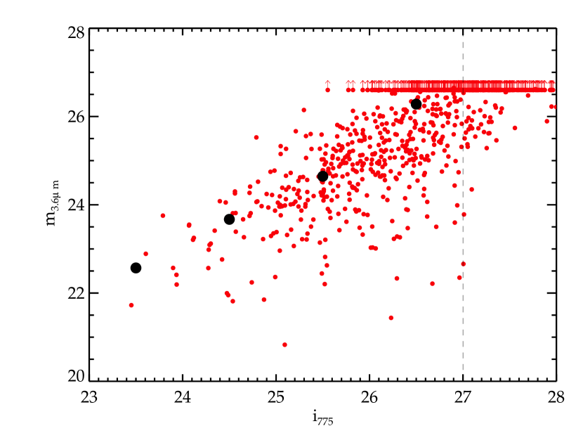
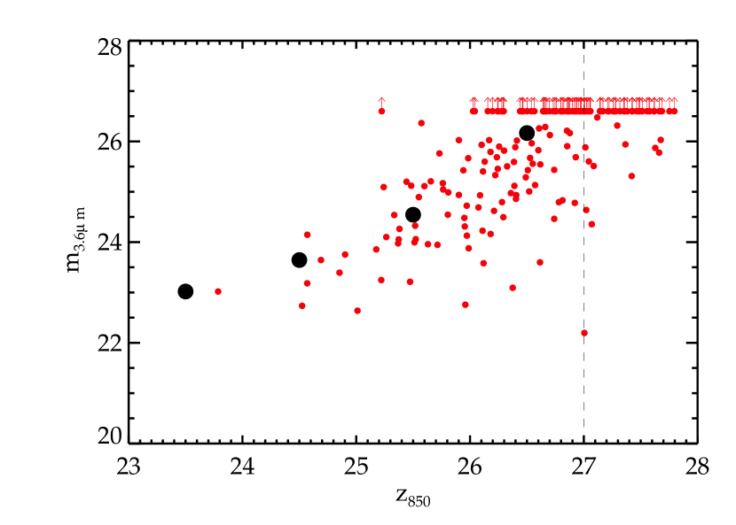
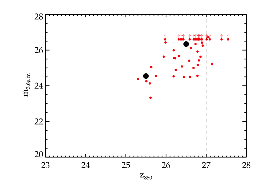
Figure 4.— Mid-infrared vs. optical flux for the B (top panel), V (middle panel), and $i^{\prime}$-drops (bottom panel). Individual galaxies are shown as small red circles; the large black circles correspond to the median 3.6$\mu$m magnitude in bins of $i_{775}$ or $z_{850}$ magnitude. The dashed vertical lines correspond to our adopted completeness limit for each dropout sample. Those objects that are brighter in the optical are on average brighter in the mid-infrared. The relationship between mid-infrared and optical flux is very similar for each of the three different redshift ranges considered.

In Figure 4, we present the relationship between the IRAC 3.6$\mu$m magnitude and $i_{775}$ or $z_{850}$ magnitude for each of our dropout samples, foreshadowing the relationship between the assembled stellar mass and the current star formation rate (uncorrected for extinction). It is not necessarily obvious that the ongoing star formation in any galaxy should bear any relation to the past star formation history, yet immediately apparent is a correlation between the average optical and mid-infrared flux: sources that are brighter in the ACS bandpasses are, on average, brighter in IRAC. Also noticeable is that the median IRAC flux for a given $i^{\prime}_{775}$ or $z^{\prime}_{850}$ flux does not change significantly over the redshift range probed by the three dropout samples. We discuss the implications of these trends in more detail in §6.

4.2. MIPS Detections

We have put considerable effort into removing low-redshift contaminants from our dataset. However, as is evident from Figure 4, the dropout samples still contain red objects, some of which are among the brightest sources detected in IRAC. Considering the fact that very massive sources (with bright IRAC fluxes) are likely much more common at $z\simeq 2$ than at $z\mathrel{\hbox to0.0pt{\lower 4.0pt\hbox{\hskip 1.0pt$\sim$}\hss}\raise 1.0pt\hbox{$>$}}4$, it is clear that these sources require more scrutiny before proceeding.

We can gain some insight into the likely redshifts of this population from 24 $\mu$m imaging with the Multiband Imaging Photometer for Spitzer (MIPS) camera (Dickinson et al. in prep.; Chary et al. in prep.). At $z\simeq 2$, the MIPS imaging passband probes the bright rest-frame 7.7 $\mu$m feature from polycyclic aromatic hydrocarbons (PAHs). As a result, dusty star-forming galaxies at $z\simeq 2$ are commonly detected with MIPS (e.g., Reddy et al. 2006). Such PAH features would not be detected in sources over the redshift range our dropouts sample (4$\mathrel{\hbox to0.0pt{\lower 4.0pt\hbox{\hskip 1.0pt$\sim$}\hss}\raise 1.0pt\hbox{$<$}}z\mathrel{\hbox to0.0pt{\lower 4.0pt\hbox{\hskip 1.0pt$\sim$}\hss}\raise 1.0pt\hbox{$<$}}$6); hence if any of our sources are detected with MIPS, it very well may indicate that they lie at $z\simeq 2$.

In order to determine what fraction of our catalog is detected at 24$\mu$m, we visually examine the MIPS data of each dropout in the Spitzer isolated sample. While the total number of dropouts with MIPS detections is small (12/800 B-drops, 3/186 V-drops, and none of the $i^{\prime}$-drops), it is not negligible. As expected, each of the sources detected with MIPS is quite red ($z^{\prime}_{850}-m_{3.6}\mathrel{\hbox to0.0pt{\lower 4.0pt\hbox{\hskip 1.0pt$\sim$}\hss}\raise 1.0pt\hbox{$>$}}2$) in addition to being bright in the IRAC bandpasses. These sources thus make up a significant fraction of the subset of our dropout samples with bright IRAC fluxes (10/25, 2/4 of those with m${}_{3.6}<$23 for the B and V-drops respectively) and are hence sure to strongly affect attempts to derive the numder density of massive galaxies.

While we consider these sources as prime low redshift candidates, it is possible that some of these lie at $z\mathrel{\hbox to0.0pt{\lower 4.0pt\hbox{\hskip 1.0pt$\sim$}\hss}\raise 1.0pt\hbox{$>$}}4$. Cross-correlating the 24$\mu$m-detected subset with our spectroscopic sample, we find that one of the three MIPS-detected V-drops has a spectroscopically confirmed redshift of $z$=4.76. Since there are few strong PAH features that fall into the 24 $\mu$m filter at this redshift, we propose that the 24 $\mu$m emission most likely comes from a dusty AGN, a conclusion consistent with the point-like morphology in the observed optical-frame. Importantly, this establishes that not all 24$\mu$m-detected dropouts are foreground objects. The MIPS-detected subsample thus places an upper limit (1.5% for the B-drops and 1.1% for the V-drops) on the number of dusty low-$z$ interlopers remaining in our samples. In subsequent sections, we will derive the evolving stellar populations of our dropout sample both with and without the 24$\mu$m detected sources.

5. Derivation of Physical Properties

We infer stellar masses for the dropout sample by fitting the latest CB07 stellar population synthesis models to the observed SEDs. These models include an improved treatment of the thermally pulsing asymptotic giant branch (TP-AGB) phase of stellar evolution, utilizing the Marigo & Girardi (2007) evolutionary tracks and the Westera et al. (2002) stellar library. In this section, we first describe the CB07 models and detail the fitting process that we use to infer the stellar masses and ages of the galaxies. We examine the effects of the TP-AGB stars on the inferred masses and ages of the dropouts by comparing the CB07 output to that from the Bruzual & Charlot (2003) population synthesis models (§5.2). We then comment on the uncertainties in the inferred properties of objects in our samples and stack the infrared photometry of the faintest sources to achieve a more reliable estimate of the average stellar populations of this subset.

5.1. CB07 Models

The CB07 models utilize 220 age steps from $10^{5}$ to $2\times 10^{10}$ yr, approximately logarithmically spaced. For each source, we do not include age steps in excess of the age of the universe implied by its photometric or spectroscopic redshift. We also exclude unphysically-low age steps (e.g., below the dynamical timescale for LBGs at high-redshift), which we take to be $\simeq 20$ Myr adopting measurements of the mean half-light radii (Bouwens et al., 2004) and typical velocity dispersions (Erb et al., 2006) of LBGs at high-redshift.

The CB07 models only include templates with the Chabrier (2003) and Salpeter (1955) initial mass functions (IMF). For consistency with previous efforts, we choose to focus on the Salpeter IMF in our analysis. The effects of utilizing a Chabrier IMF have been discussed in detail elsewhere, including our previous work (Eyles et al., 2005; Stark et al., 2007).

We use the high resolution (FWHM 3 Å) and 1 Å pixels evenly-spaced over the wavelength range of 3300 Å to 9500 Å (unevenly spaced outside this range). From the full range of metallicities offered by the code, we considered both solar and 0.2 Z_⊙ models. From several star formation histories available, we utilize the constant star formation history and exponentially decaying ($\tau$) SFR models with e-folding decay timescales $\tau$=100 and 300 Myr. We also utilize a model with a linearly increasing star formation rate, with a slope set to match the observed brightening in the UV LF between $z\simeq 6$ and 4 (0.74 mag at 1500 Å  over $\simeq 620$ Myr). The CB07 spectra are normalized to an SFR of $1\,\rm{M_{\odot}}\,{\rm yr}^{-1}$ for the continuous star formation model. For the exponential decay models, the galaxy mass is normalized to M $\longrightarrow$ 1 M_⊙ as t $\longrightarrow$ $\infty$.

We also consider the effects of dust on the integrated SEDs, adopting the reddening model of Calzetti (1997). At each age step, the model SED was folded in with each of five different reddening curves corresponding to color excesses of E(B-V)=0.0, 0.03, 0.1, 0.3, 1.0.

For each of the galaxies in our sample, the model SEDs were interpolated onto each of the filters’ wavelength scales after correcting the latter to the rest-frame wavelengths using the redshift appropriate for each object. Rather than simultaneously fitting the mass, age, dust, and redshift, we fixed the redshift at the best-fit photometric redshift specified by BPZ. Where possible, we instead utilized spectroscopic redshifts. We discuss the effects of holding the redshift fixed later in §5.3. To assess the uncertainty in the inferred parameters (e.g., mass, age, dust) due to redshift error, we perform the SED fitting at three redshifts: $z=z_{\rm{phot}}-0.25,z_{\rm{phot}},z_{\rm{phot}}+$0.25.

To account for Ly$\alpha$ forest absorption, we decrement the flux shortward of 1216 Å  (rest-frame) by a factor of $\exp[-(\rm{1}+z)^{3.46}]$ (Madau, 1995). We further assume the flux shortward of 912 Å  (rest-frame) is zero due to Lyman-limit absorption.

The resulting template SEDs are folded through each of the filter transmission curves to produce optical, near-IR, and mid-IR magnitudes for each model. Comparing the observed magnitudes and their associated errors to the derived model magnitudes, we compute a reduced $\chi^{2}$ value for each set of parameters (age, E(B-V), normalization). For individual sources, non-detections were set to the 1$\sigma$ detection limit and the flux error was set at 100% (we also consider the average properties of this faint sample via a stacking analysis in §5.2)

The fitting routine returned the parameters for each model which were the best-fit to the broadband photometry (i.e., minimized the reduced $\chi^{2}$). In addition to selecting those parameters which provide the best-fit, we also compute the range of ages, normalizations, and $E(B-V)$ values that result in an SED with reduced $\chi^{2}$ values within $\Delta\chi_{reduced}^{2}$=1 of the minimum value; we take these as the 1-$\sigma$ uncertainties associated with each parameter. This normalization was then converted to the appropriate units and subsequently used to calculate the corresponding best-fit stellar and total mass (and the corresponding 1$\sigma$ errors). The conversion factor between normalization and mass for a given age and star formation history was obtained from the ’4color’ files in the CB07 population synthesis output.

5.2. The Effect of TP-AGB stars on Inferred Properties at $z\mathrel{\hbox to0.0pt{\lower 4.0pt\hbox{\hskip 1.0pt$\sim$}\hss}\raise 1.0pt\hbox{$>$}}4$

The TP-AGB stars contribute significantly to the integrated rest-frame near-infrared light. Maraston (2005) has shown that if the contribution from this phase of evolution is underestimated for galaxies at $z\simeq 2$, the stellar masses and ages inferred from models are typically overestimated. Note that this is not necessarily the case at $z\mathrel{\hbox to0.0pt{\lower 4.0pt\hbox{\hskip 1.0pt$\sim$}\hss}\raise 1.0pt\hbox{$>$}}4$, since at these redshifts the first two IRAC channels only probe as far redward as the rest-frame optical, where the contribution from TP-AGB stars is less dominant than the rest-frame near-infrared. In this section, we investigate the effect of the TP-AGB stars on the inferred properties of the B, V, and $i^{\prime}$-drops by comparing the model output of CB07 and BC03 models.

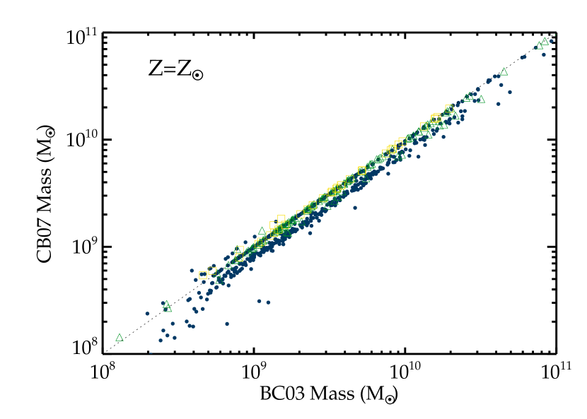
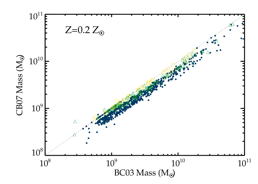
Figure 5.— Comparison of the model output from Bruzual & Charlot (2003) (BC03) and the updated models presented in Bruzual 2007 (CB07) which now include the contribution of TP-AGB stars. The upper panel shows B-drops (blue circles), V-drops (green triangles), and $i^{\prime}$-drops (yellow squares) for a solar metallicity $\tau$=100 Myr exponential decay model. The lower panel is identical but with sub-solar (Z=0.2 $Z_{\odot}$) metallicity. The dotted line in both panels indicates the 1-to-1 relationship between the BC03 and CB07 mass. The discrepancy between the BC03 and CB07 models increases at lower redshifts and lower metallicities.

In Figure 5a, the stellar masses of the B, V, and $i^{\prime}$-drop samples inferred from BC03 and CB07 are plotted against one other for solar metallicity. In computing the masses and ages, we fix the redshift at the derived photometric redshift and the color excess is fixed to $E(B-V)$=0. In spite of the addition of TP-AGB stars, the inferred masses from BC03 and CB07 are in very good agreement. The median stellar mass of the BC03 $i^{\prime}$-drops is less than 1% greater than that for the CB07 $i^{\prime}$-drops. As expected the effect of TP-AGB is more pronounced at lower redshifts, but nevertheless we still find only a 9% difference between the median of the BC03 and CB07 B-drop samples.

At subsolar metallicity, the contribution from TP-AGB stars is significant ($\mathrel{\hbox to0.0pt{\lower 4.0pt\hbox{\hskip 1.0pt$\sim$}\hss}\raise 1.0pt\hbox{$>$}}$20-30% of luminosity for 1.3 Gyr instantaneous burst) in the rest-frame optical (Bruzual, 2007); hence, we expect the CB07 models to return lower masses than the BC03 models for the 0.2 Z_⊙ templates. Indeed, we find that in each dropout sample the variations between the two models is more extreme than in the solar metallicity case (Figure 5b). In the most discrepant case (the B-drops), the median mass inferred from the BC03 models is $\simeq 30$% greater than that inferred from CB07.

5.3. Systematic Uncertainties in Derived Properties

Before examining the results in detail, we explore the reliability with which we can determine the stellar populations of $z\mathrel{\hbox to0.0pt{\lower 4.0pt\hbox{\hskip 1.0pt$\sim$}\hss}\raise 1.0pt\hbox{$>$}}4$ galaxies. There is ample discussion of the systematic uncertainties inherent in population synthesis modeling in the literature (e.g., Papovich et al. 2001; Shapley et al. 2001; Yan et al. 2005; Eyles et al. 2005; Shapley et al. 2005). We direct the reader to these works for detailed discussion and only provide a brief discussion below on the typical uncertainties in the inferred masses, ages, and extinction for our dropout samples.

First we must consider whether fixing the redshift at a single value biases our determination of the mass and its associated uncertainty. To test this, we compute the best-fit parameters for the small subset of sources with spectroscopic redshifts using two different methods: 1) fixing the redshift at the photometric redshift determined by BPZ and 2) allowing the redshift to float simultaneously with mass, age, and dust. Comparing these to the parameters inferred when the redshift has been fixed at its true spectroscopic value gives some indication of the error that may be introduced by not allowing the redshift to float. We find that the best-fit stellar masses inferred by method 1 (fixing the redshift at its BPZ photometric redshfit) are similar to those determined when the redshift is fixed at its spectroscopic value (the standard deviation in the fractional difference between the two mass estimates is 17%). Varying the redshift simultaneously with other parameters does not result in better agreement with the masses inferred from the spectroscopic redshifts (the standard deviation in the fractional difference between the two mass estimates is 19%). Moreover, we find that the uncertainty in the stellar mass that is found by perturbing the redshift by $\Delta$z=$\pm$0.25 from its best-fit BPZ photometric redshift and allowing the dust and age to vary (42% error) is very similar to that determined by allowing the redshift to float simultaneously with dust and age (48% error). These results suggest that our method of using fixed redshifts in our SED fitting analysis will not strongly bias the mass determinations or decrease the inferred mass error.

We now move on to quantify the uncertainty in the derived parameters for sources in our dropout samples. The SED fitting procedure is clearly most effective at fitting sources that are bright enough to be detected with sufficiently high S/N ($\simeq 10$) in the rest-UV and rest-optical. For the bright $z^{\prime}_{850}=24.3$ dropout presented in Figure 6 (typical of bright B-drops in our sample), acceptable fits (within $\Delta\chi_{reduced}^{2}$=1 of the best-fit) are found for models with ages between 180 and 321 Myr, color excesses between E(B-V)=0.0 and 0.1, and stellar masses between 2.0 and 2.8$\times$10¹⁰ M_⊙. If we allow the redshift to vary by $\pm 0.25$ and consider the range of models that produce a reduced $\chi^{2}$ within 1 of minimum reduced $\chi^{2}$ at the central BPZ photometric redshfit, the inferred stellar masses vary by less than 5% and ages change by less than $\simeq 30$%. Variations in the form of the star formation history do change the absolute values quoted above (see Shapley et al. 2005 for detailed discussion), with best fit stellar masses increasing by 35% and ages reaching 1.4 Gyr for a constant star formation model. Nevertheless the relative stellar masses and ages within our samples should be reasonably well determined for equally bright dropouts, unless the star formation history varies considerably within the sample.

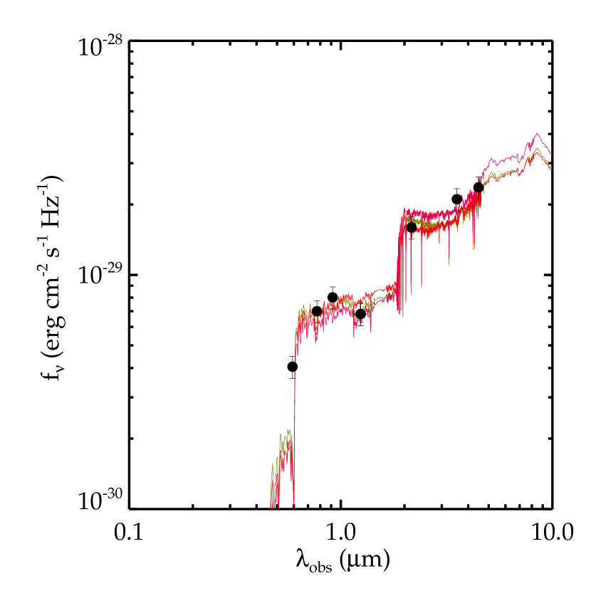
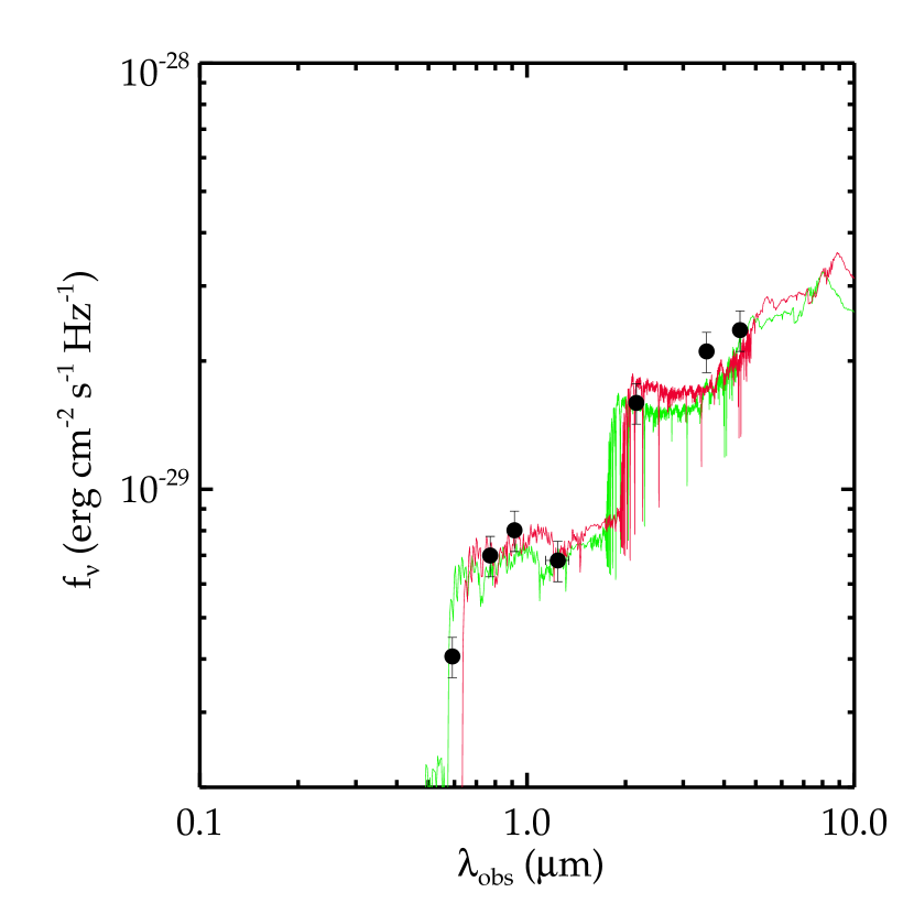
Figure 6.— SED of a B-drop (typical of bright sources in our sample) compared with a range of CB07 model SEDs that fit the data. Top: Adopting a model with an exponentially decaying star formation history with $\tau$=100 Myr, we find the SED is best fit by an age of 286 Myr and a stellar mass of 2.3$\times$10¹⁰ M_⊙ with E(B-V)=0 (green curve). Allowing the dust content to vary, we find acceptable fits for stellar masses ranging between 2.0 and 2.8$\times$10¹⁰ M_⊙ and ages between 180 and 321 Myr. The model with the lower mass and age is shown as the red curve (and has E(B-V)=0.1); the model that provides the upper bound to the mass and age is shown in purple (and has E(B-V)=0). Bottom: Perturbing the photometric redshift by $\Delta z=\pm$0.25, we find that the higher redshift solution (red curve) provides a significantly less accurate fit to the data ($\Delta\chi_{reduced}^{2}$= 3.06) than that provided by the $\Delta z=-0.25$ SED (green curve) and the SED derived using the best fit photo-$z$. The inferred stellar mass in the lower redshift model (2.3$\times$10¹⁰ M_⊙) is within 5% of the best-fit value at the best-fit BPZ photometric redshift and the inferred age (203 Myr) is within 30%.

Extracting robust information from the SEDs of faint dropouts is more difficult than for the bright sources discussed above, largely because the near and mid-infrared datasets are not deep enough to detect very faint objects. Sources that are undetected in IRAC have a median mass of 2$\times$10⁸ M_⊙ and age of 80 Myr for the $\tau$=100 Myr exponential decay model, but their SEDs have acceptable masses and ages spanning a factor of 10. In general, we find that in order to achieve reasonably reliable masses for individual objects, we must limit our sample to those dropouts with $\mathrel{\hbox to0.0pt{\lower 4.0pt\hbox{\hskip 1.0pt$\sim$}\hss}\raise 1.0pt\hbox{$>$}}10^{9.5}$ M_⊙. In Figure 7, we present the SED of a typical object near this mass limit (best fit stellar mass of 5$\times$10⁹ M_⊙); acceptable CB07 fits for the $\tau$=100 Myr exponentially decay star formation history are found using models with stellar masses between 2.4 and 7$\times$10⁹ M_⊙, ages between 21 Myr and 360 Myr, and color excesses between $E(B-V)=0$ and $0.3$. While the data allow a wide range of ages and dust extinctions, the stellar mass can be determined reasonably well.

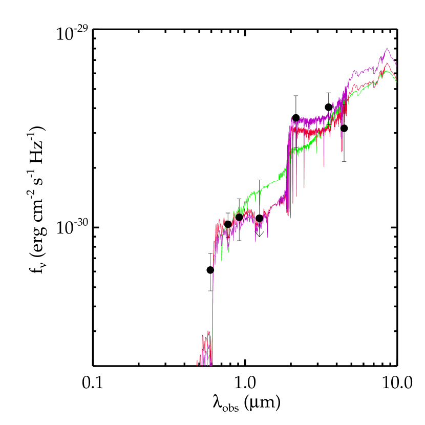
Figure 7.— SED of a B-drop typical of sources at the adopted 10^9.5 M_⊙ stellar mass limit. Adopting a model with an exponentially decaying star formation history with $\tau$=100 Myr, we find the SED is best fit by an age of 320 Myr and a stellar mass of 4.8$\times$10⁹ M_⊙ with E(B-V)=0 (red curve). Allowing the dust content to vary, we find acceptable fits for stellar masses ranging between 2.4 and 6.7$\times$10⁹ M_⊙ and ages between 21 and 360 Myr. The model with the lower mass and age is shown as the green curve (and has E(B-V)=0.3); the model that provides the upper bound to the mass and age is shown in purple (and has E(B-V)=0).

To obtain an estimate of the average properties of galaxies less massive than this limit, we perform a stacking analysis on the low S/N infrared data. For each of the three dropout samples, we select all sources that are undetected and unconfused at 3.6 $\mu$m, amounting to 171 B-drops, 29 V-drops, and 17 $i^{\prime}$-drops. For each of the dropout samples, the median $z^{\prime}_{850}$-band magnitude of this faint subset is $\simeq 26.7$. Following the techniques discussed in Eyles et al. (2007), we stack the IRAC data of each of the undetected dropouts (excluding those with $\mathrel{\hbox to0.0pt{\lower 4.0pt\hbox{\hskip 1.0pt$\sim$}\hss}\raise 1.0pt\hbox{$<$}}65$ ksec of exposure time) using a median combine with no weighting to reduce the effect of contamination by neighboring sources. We follow a very similar approach in stacking the near-IR data, limiting our sample to the objects in GOODS-S given the slightly deeper images in that field.

Table 1Photometry of Stacked Images

J	$K_{s}$	m3.6μm	m4.5μm
B-drops ($z\simeq 4$)
27.03(0.15)	26.51(0.15)	26.79(0.31)	27.29 (0.17)
V-drops ($z\simeq 5$)
26.7(0.34)	26.55(0.48)	26.89(0.21)	27.71(0.57)
$i^{\prime}$-drops ($z\simeq 6$)
26.69(0.32)	26.43(0.42)	27.23(0.33)	27.64(0.87)

Note. — The photometric errors of the stacked images are provided in parenthesis next to the measured magnitudes.

The stacking procedure described above resulted in near and mid-IR detections for the B, V, and $i^{\prime}$-drops (see Table 1 for photometry). The model fit to the composite faint B-drop subsample SED is displayed in Figure 8. For the exponential-decay ($\tau=100$ Myr) model, the best-fit solar metallicity model has a stellar mass of 1.7$\times$ 10⁸ M_⊙ (acceptable fits range between 6.2$\times$10⁷ and 3.2$\times$10⁸ M_⊙) and age of 48 Myr. We find similar best fitting models for the stacked V-drops (1.5$\times$10⁸ M_⊙ and 25 Myr) and $i^{\prime}$-drops (2.6$\times$10⁸ M_⊙ and 38 Myr). In all cases, the SED is actually slightly better fit by a sub-solar metallicity model ($\Delta\chi^{2}\simeq 0.4$-0.6) in agreement with the results of Eyles et al. (2007); however, the returned stellar masses and ages do not change significantly from those obtained using the solar metallicity models (Figure 8). Importantly, the inferred masses and ages of the stacked SEDs are consistent with what we would have obtained by merely taking the average of the masses and ages of the individual galaxies included in the stack, suggesting that in spite of the large uncertainties, we can still use the inferred properties of this faint subset and be confident that the average properties are robust.

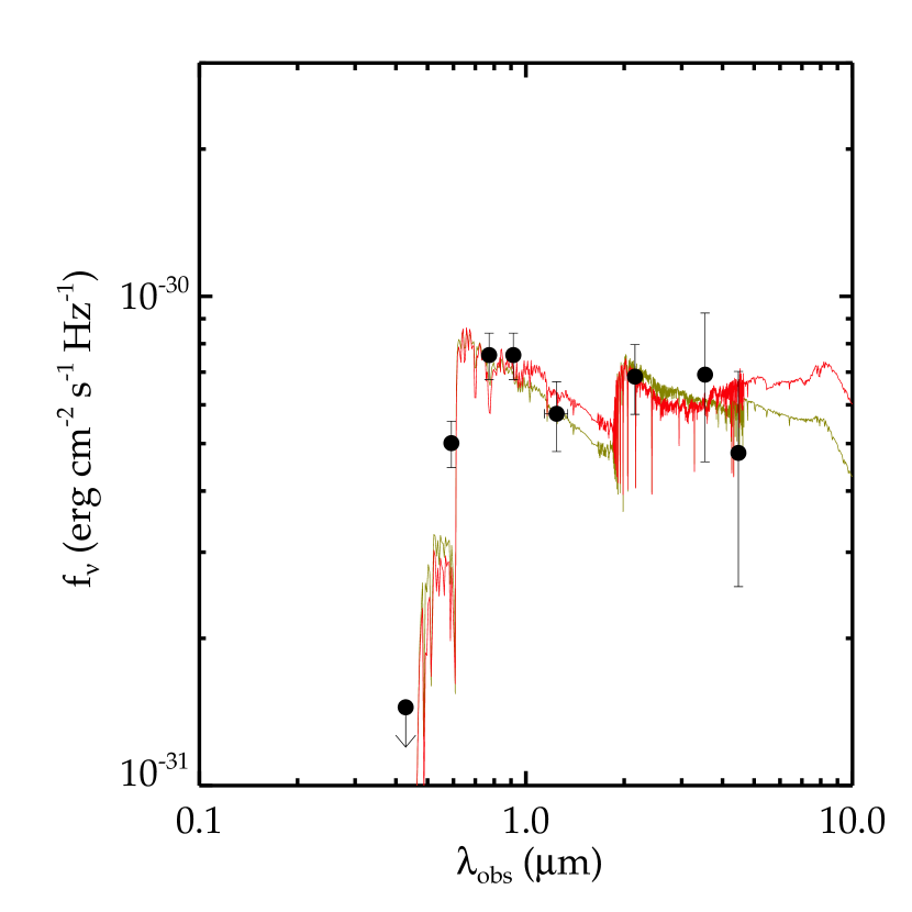
Figure 8.— Fit to composite SED of faint B-drop stack. The best-fitting exponential decay $\tau$=100 Myr model with solar metallicity (red SED) has a stellar mass of 1.7$\times$ 10⁸ M_⊙ and age of $\simeq 50$ Myr. Using a subsolar metallicity, Z=0.2$Z_{\odot}$, template (green SED), we find a marginally better fit to the data ($\Delta\chi^{2}$= 0.5) with similar inferred masses and ages (2.4$\times$10⁸ M_⊙ and $\simeq 70$ Myr).

6. New Insight into the History of High Redshift Star Formation

One of the most basic questions in the study of galaxy formation is how galaxies grow over cosmic time. Observations have now revealed vast populations of vigorously assembling galaxies at $z\mathrel{\hbox to0.0pt{\lower 4.0pt\hbox{\hskip 1.0pt$\sim$}\hss}\raise 1.0pt\hbox{$>$}}4$, but it remains unclear how star formation proceeds in these objects. On one hand it is possible that $z\mathrel{\hbox to0.0pt{\lower 4.0pt\hbox{\hskip 1.0pt$\sim$}\hss}\raise 1.0pt\hbox{$>$}}4$ LBGs assemble their mass at a constant rate, growing continuously between $z\simeq 6$ and 4. This “steady growth” scenario may be expected if high redshift galaxies are constantly fueled by cold gas which is in turn rapidly converted into stars. Alternatively, galaxies may undergo punctuated star formation episodes lasting only several hundred Myr or less, such that those LBGs seen at $z\simeq 5$, for example, are not necessarily related to those seen at later times (e.g., at $z\simeq 4$) or at earlier times (e.g., $z\simeq 6$). This “independent generations” scenario could arise if relatively rare events (e.g., major mergers, instabilities) are predominantly responsible for sparking luminous star formation at $z\mathrel{\hbox to0.0pt{\lower 4.0pt\hbox{\hskip 1.0pt$\sim$}\hss}\raise 1.0pt\hbox{$>$}}4$, or alternatively if feedback effects act to shut off star formation after several hundred Myr.

Testing the validity of these scenarios has proven difficult with rest-UV observations alone, as these studies only probe recent star formation activity, revealing little about the physical properties of the galaxies being assembled. But it is the evolution of such properties (i.e., stellar mass, age, dust) which can potentially illuminate the relationship between galaxies at $z\simeq 4$ and $z\simeq 6$. If the LBGs seen at $z\simeq 4$ have been forming stars at a constant rate since $z\simeq 5-6$, then the higher redshift objects of a given luminosity should appear as “scaled-down” versions of those at $z\simeq 4$, with lower masses, ages, and reduced dust content. In contrast, if the LBG population at $z\simeq 4$ is dominated by galaxies which were either quiescent or forming stars less vigorously at $z\simeq 5$ and 6, then we would not necessarily expect the stellar populations to show signs of growth between the two different epochs.

In this section, we attempt to distinguish between these various scenarios by exploring the evolution of the relationship between the stellar mass and UV luminosity (hereafter the M_⋆-M₁₅₀₀ relation). For a given galaxy, this diagnostic illuminates the ratio of the past and present star formation. At lower redshifts, this relationship has been used effectively to constrain stellar mass growth in galaxies (Noeske et al., 2007; Daddi et al., 2007). Studying the redshift evolution of this relation for a large sample of high redshift dropouts reveals whether the typical specific star formation rate (SFR/M_⋆) and stellar mass of UV luminous galaxies changes significantly between $z\simeq 4$ and 6, allowing new constraints to be placed on the past star formation history.

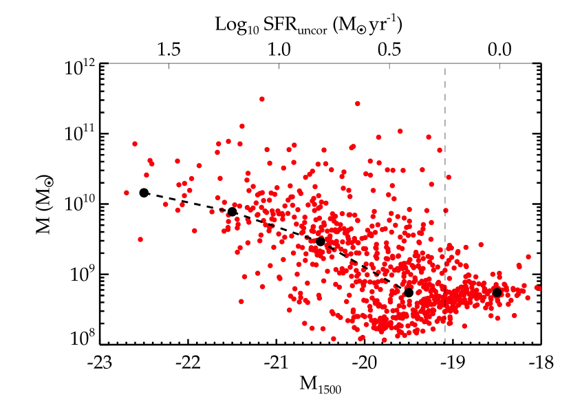
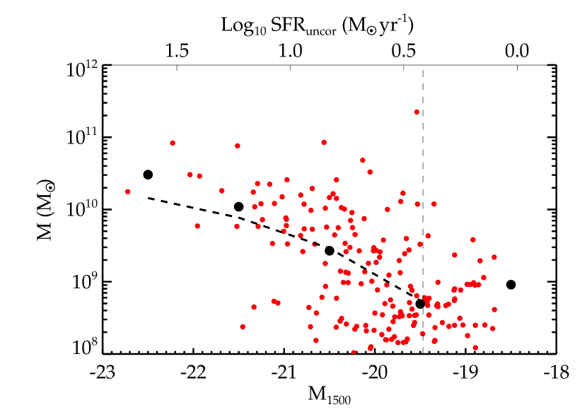
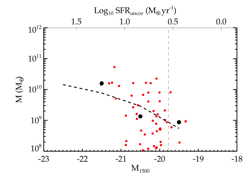
Figure 9.— Stellar mass vs. absolute magnitude at 1500Å (uncorrected for dust extinction) over $z\simeq 4-6$. Small red circles correspond to inferred stellar masses and rest-UV absolute magnitudes for individual B-drops (top), V-drops (middle) and $i^{\prime}$-drops (bottom) assuming a $\tau=100$ Myr exponential decay model. The dark solid circles are the median stellar mass in each magnitude bin. The relationship at $z\simeq 4$ is overlaid on the $z\simeq 5$ and $z\simeq 6$ panels as a black solid dashed line. The vertical solid lines represent the adopted completeness limits for each sample. The median stellar mass increases monotonically with M₁₅₀₀ in each dropout sample; however at a fixed M₁₅₀₀, the median stellar mass does not decrease significantly with increasing redshift, as may be expected in simple steady growth models.

In Figure 9, we present the inferred stellar masses of the B, V, and $i^{\prime}$-drops as a function of absolute magnitude at rest-frame 1500 Å  (M₁₅₀₀). We compute the absolute magnitude from the observed $i^{\prime}$-band magnitudes for the B-drops, and the $z^{\prime}$-band magnitudes for the V- and $i^{\prime}$-drops using photometric redshifts where spectroscopic confirmation is not available. Ideally we would correct the absolute magnitudes for dust extinction, but doing so can introduce considerable error into the relation. For example, using the Meurer relation (Meurer et al., 1999) we find that the extinction at 1600 Å, A₁₆₀₀, is related to the rest-UV color for dropouts at $z=4$ by the following relation: A₁₆₀₀=0.415 + 10.9($i^{\prime}_{775}$-$z_{850}$). This indicates that photometric uncertainties as small as 0.1 mags in the rest-UV color translate to more than 1 mag of uncertainty in the extinction correction. Further error arises from uncertainty in the redshifts and, to a lesser extent, the ages of the dropouts, both of which alter the relation between extinction and color derived above. Together, these sources of error would undoubtedly add significant random scatter to the M_⋆-M₁₅₀₀ relation, quite possibly washing out any trends that may exist with luminosity or redshift. We thus limit our analysis to the relationship between stellar mass and emerging luminosity (i.e., the luminosity inferred from the flux that escapes the galaxy) and comment below on the specific effects that not correcting for dust extinction may have on our results.

For each of the dropout samples, we find that the median stellar mass increases monotonically with increasing emerging UV luminosity (forming a so-called “main-sequence”), albeit with very significant scatter in each magnitude bin. Similar relations are commonly seen at lower redshifts (e.g., Daddi et al. 2007) and are predicted to arise at high redshift in hydrodynamic simulations (e.g., Finlator et al. 2006). In the idealized scenario in which the bright dropout population emerges at $z\simeq 6.5$ and steadily grows in stellar mass via a constant star formation rate (with no new galaxies emerging as luminous dropouts), we would expect the typical dropout stellar masses to increase by a factor of $\simeq 7$ in the time between $z\simeq 6$ (when the galaxy has an age of $\simeq 90$ Myr) and $z\simeq 4$ (when the galaxy has an age of $700$ Myr).

Table 2Evolution of Galaxy Properties over 4$\mathrel{\hbox to0.0pt{\lower 4.0pt\hbox{\hskip 1.0pt$\sim$}\hss}\raise 1.0pt\hbox{$<$}}$z$\mathrel{\hbox to0.0pt{\lower 4.0pt\hbox{\hskip 1.0pt$\sim$}\hss}\raise 1.0pt\hbox{$<$}}$6

MUV	Num	M⋆ ($\tau$=100)	M⋆ (CSF)	Age
(mag)		(108 M⊙)	(108 M⊙)	(Myr)
B-drops ($z\simeq 4$)
-22.5	15	144 (31-410)	223	180
-21.5	73	77 (24-380)	114	203
-20.5	227	29 (4.0-130)	38	181
-19.5	370	5.5 (2.0-42)	7.3	143
V-drops ($z\simeq 5$)
-22.5	3	304 (180-830)	520	286
-21.5	20	109 (5.4-234)	112	227
-20.5	67	27 (2.2-158)	36	181
-19.5	…	…	…	…
$i^{\prime}$-drops ($z\simeq 6$)
-22.5	0	…	…	…
-21.5	8	160 (24-530)	226	286
-20.5	41	13 (1.3-90)	27	102
-19.5	…	…	…	…

Note. — The stellar masses and ages are inferred from models using a Salpeter IMF and solar metallicity. In column 3, we present the median stellar masses (and the range of masses spanned by the middle 80% of the distribution) determined from an exponentially-declining star formation history with $\tau$=100 Myr. In column 4, we provide the median stellar masses inferred assuming a constant star formation history. In column 5, we present the median ages inferred for the $\tau$=100 Myr models.

Examining the top, middle, and bottom panels of Figure 9, we do not see such a systematic increase in the normalization of the M_⋆-M₁₅₀₀ relation between $z\simeq 6$ and $4$ (Table 2). While the lowest luminosity bin above our completeness limit may show some signs of marginal stellar mass growth between $z\simeq 6$ and 5 (i.e., a $\times 1.3-2.0$ increase in the median stellar mass), this same bin shows no growth between $z\simeq 5$ and 4 in spite of the improved mass estimates and statistics available at the lower redshifts. The most luminous bins actually show a slight decrease in the average stellar mass with cosmic time. As shown in Table 2, the absence of a systematic increase in the average stellar masses is not strongly dependent on the chosen star formation history. Overall these results seem to imply that the ratio of median stellar mass to emerging UV luminosity does not evolve significantly for LBGs over $z=4-6$. A galaxy with a given M₁₅₀₀ at $z\simeq 6$ will, on average, have the same assembled mass (to within a factor of $\simeq 2$) as a galaxy seen at $z\simeq 4$ with the same M₁₅₀₀. This suggests that the specific star formation rate evolves weakly over $4\mathrel{\hbox to0.0pt{\lower 4.0pt\hbox{\hskip 1.0pt$\sim$}\hss}\raise 1.0pt\hbox{$<$}}z\mathrel{\hbox to0.0pt{\lower 4.0pt\hbox{\hskip 1.0pt$\sim$}\hss}\raise 1.0pt\hbox{$<$}}6$, indicating that the typical duration of past star formation for a galaxy of a given luminosity does not vary significantly between $z\simeq 6$ and 4.

While the inclusion of a dust correction would shift the M_⋆-M₁₅₀₀ relation brightward (i.e., to the left in Figure 9), it would likely not lead to an increase in the normalization of the M_⋆-M₁₅₀₀ relation over time. As has been shown elsewhere (e.g., Stanway et al. 2005; Bouwens et al. 2007) galaxies at M${}_{1500}<-$19.8 do potentially become marginally dustier between $z\simeq 6$ and 4 which would cause the $z\simeq 4$ M_⋆-M₁₅₀₀ relation to shift slightly more than the $z\simeq 5$ and 6 relations. Since a relative shift brightward is roughly the same as a shift toward lower stellar masses at fixed M₁₅₀₀, this would actually have the effect of slightly decreasing the normalization of the M_⋆-M₁₅₀₀ relation over the $4\mathrel{\hbox to0.0pt{\lower 4.0pt\hbox{\hskip 1.0pt$\sim$}\hss}\raise 1.0pt\hbox{$<$}}z\mathrel{\hbox to0.0pt{\lower 4.0pt\hbox{\hskip 1.0pt$\sim$}\hss}\raise 1.0pt\hbox{$<$}}6$ redshift range.

6.1. Testing the Steady Growth Scenario

We now attempt to place the M_⋆-M₁₅₀₀ relation presented in Figure 9 in the context of the steady growth scenario discussed at the outset of this section. To approximate this scenario, we assume that galaxies follow a constant star formation rate. Using solar metallicity templates and allowing the dust content to freely vary, we find that the typical implied star formation lifetimes of the B-drops are in excess of 700 Myr in the two brightest bins (Figure 10), implying that the precursors of the majority of B-drops would have been equally luminous in V and $i^{\prime}$-drop samples. We therefore would have expected to see a steady decline in the typical stellar masses and ages of UV luminous galaxies at $z\simeq 5$ and 6. The fact that the $z\simeq 6$ LBGs are, on average, quite similar in mass and age to those of similar luminosity at $z\simeq 4$ suggests that the precursors of most of the $z\simeq 4$ LBGs were not at the same UV luminosity (or perhaps were even quiescent) at $z\simeq 6$. Similar arguments are arrived at by considering the observed UV luminosity function (UV LF) of the dropouts over this redshift interval (Bouwens et al., 2007). The large implied ages mentioned above combined with the constant past star formation rate suggest that the number density of galaxies at a given M₁₅₀₀ should not fall off significantly with increasing redshift, in sharp contrast to the observed trend. Indeed, the distribution of ages implied by this constant star formation rate scenario is such that the number density of galaxies at M${}_{1500}<-21.5$ should not decrease by more than a factor of $\simeq 2$ over $4\mathrel{\hbox to0.0pt{\lower 4.0pt\hbox{\hskip 1.0pt$\sim$}\hss}\raise 1.0pt\hbox{$<$}}z\mathrel{\hbox to0.0pt{\lower 4.0pt\hbox{\hskip 1.0pt$\sim$}\hss}\raise 1.0pt\hbox{$<$}}6$, in marked contrast to the observed $\times$10 decline in the bright end of the luminosity function at M${}_{1500}\mathrel{\hbox to0.0pt{\lower 4.0pt\hbox{\hskip 1.0pt$\sim$}\hss}\raise 1.0pt\hbox{$<$}}-21.5$ over this redshift interval (Bouwens et al., 2007).

We therefore argue that in order to explain the constancy in the M_⋆-M₁₅₀₀ relationship and the decline in the UV luminosity function, we require a star formation model that implies that a significant fraction of UV-luminous galaxies at $z\mathrel{\hbox to0.0pt{\lower 4.0pt\hbox{\hskip 1.0pt$\sim$}\hss}\raise 1.0pt\hbox{$>$}}4$ emerged at their present UV luminosity recently enough such that they would not have been visible as dropouts at the same UV luminosity just $\simeq 300$ Myr earlier (e.g., the time corresponding to $\Delta z\simeq 1$ at $4\mathrel{\hbox to0.0pt{\lower 4.0pt\hbox{\hskip 1.0pt$\sim$}\hss}\raise 1.0pt\hbox{$<$}}z\mathrel{\hbox to0.0pt{\lower 4.0pt\hbox{\hskip 1.0pt$\sim$}\hss}\raise 1.0pt\hbox{$<$}}6$). With a constantly increasing flux of newly luminous galaxies, the galaxy population at each epoch would likely be dominated by relatively young ($\mathrel{\hbox to0.0pt{\lower 4.0pt\hbox{\hskip 1.0pt$\sim$}\hss}\raise 1.0pt\hbox{$<$}}300$ Myr) objects. Hence the main sequence of the M_⋆-M₁₅₀₀ relation would not necessarily grow significantly with cosmic time as one would expect in the steady growth scenario.

We note that this requirement of a young population is not inherently inconsistent with constant, sustained star formation in galaxies. Indeed, if each of the $z\mathrel{\hbox to0.0pt{\lower 4.0pt\hbox{\hskip 1.0pt$\sim$}\hss}\raise 1.0pt\hbox{$>$}}4$ dropout populations is dominated in number by newly emerged luminous galaxies, it is possible that systems which are UV luminous at $z\simeq 6$ remain luminous to $z\simeq 4$, but make up such a small fraction (by number) of the $z\simeq 4$ LBG population so as not to affect the main sequence of the M_⋆-M₁₅₀₀ relation. The key problem with this picture, as hinted by our results above, is that constant star formation models struggle to produce young enough ages to be consistent with the need to have each epoch (i.e. $z\simeq 4$) dominated by systems that weren’t present at the previous epoch (i.e. $z\simeq 5$).

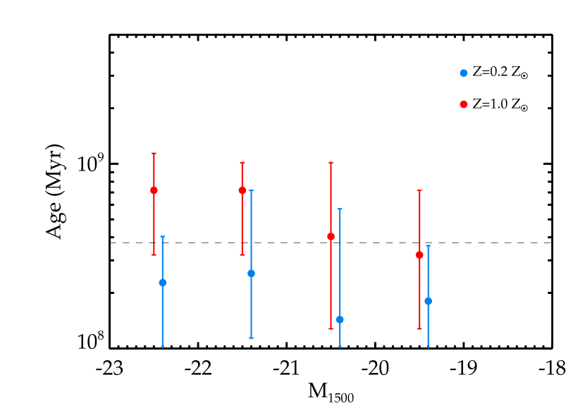
Figure 10.— Ages inferred for B-dropout sample from constant star formation scenario as a function of absolute magnitude at 1500 Å (uncorrected for dust). The solid red circles give the median inferred age for CB07 models with solar metallicity while the blue circles give the median ages for models with 20% solar metallicity. The error bars on each datapoint correspond to the 25th (lower bar) and 75th (upper bar) percentile in the distribution of ages in each absolute magnitude bin. The horizontal dashed line denotes the amount of time spanned between $z\simeq 4$ and 5. Thus if the inferred ages are above the dashed line, it indicates a large fraction of the B-drops began forming stars beyond $z\simeq 5$, implying an abundant precursor population with scaled-down masses relative to those measured at $z\simeq 4$. The lack of evolution in the normalization of the M_⋆-M₁₅₀₀ relationship over $z\simeq 4-6$ (Figure 9) casts doubt on this scenario.

It is valuable to consider the systematic uncertainties that could arise following degeneracy in derving both age and dust extinction measures from our photometric data. If our dust estimates are systematically too low, then the ages quoted above are likely overestimates. In addition, if we adopt lower metallicity templates in our models (e.g., 0.2 Z_⊙) as may be appropriate for $z\mathrel{\hbox to0.0pt{\lower 4.0pt\hbox{\hskip 1.0pt$\sim$}\hss}\raise 1.0pt\hbox{$>$}}4$, we find ages that are a factor of $\simeq 2$ lower than those in Table 2 (Figure 10). Thus while the relatively large ages implied by the constant star formation rate scenario do cause some tension with the observed evolution in the M_⋆-M₁₅₀₀ relation and UV LF, there are feasible steady growth scenarios that are potentially consistent with the observations. Improved spectroscopic completeness and infrared photometry will soon enable us to lessen the uncertainty in the dust content and to provide estimates of the metallicities, both of which will help test the feasibility of these scenarios.

A possible variant on the “steady growth” scenario is a situation where star formation grows increasingly vigorous as galaxies grow in mass at early times. While such star formation histories are not typically used in fitting high redshift galaxies, they are predicted in SPH simulations (Finlator et al., 2006) and have successfully been used to infer the properties of two $z\mathrel{\hbox to0.0pt{\lower 4.0pt\hbox{\hskip 1.0pt$\sim$}\hss}\raise 1.0pt\hbox{$>$}}6$ galaxies (Finlator et al., 2007). In this case, galaxies would grow along the “main sequence” of the M_⋆-M₁₅₀₀ relation of Figure 9, which results in little evolution of the normalization of the M_⋆-M₁₅₀₀ relation over 4$\mathrel{\hbox to0.0pt{\lower 4.0pt\hbox{\hskip 1.0pt$\sim$}\hss}\raise 1.0pt\hbox{$<$}}z\mathrel{\hbox to0.0pt{\lower 4.0pt\hbox{\hskip 1.0pt$\sim$}\hss}\raise 1.0pt\hbox{$<$}}6$, similar to the observed trend. This picture is also able to explain the observed luminosity function evolution. If galaxies in the luminosity range probed by our study steadily brighten by $\simeq 0.7$ mag at 1500 Å  in the $\simeq 620$ Myr between $z\simeq 6$ and 4 (matching the evolution seen in the characteristic UV luminosity, M${}^{\star}_{\rm{UV}}$), then this scenario would be fully consistent with the observed evolution in the UV luminosity function.

Importantly, a significant obstacle for each of the “steady growth” scenarios described above comes from observations of the clustering of dropouts at $z\mathrel{\hbox to0.0pt{\lower 4.0pt\hbox{\hskip 1.0pt$\sim$}\hss}\raise 1.0pt\hbox{$>$}}4$ (Ouchi et al., 2004; Lee et al., 2006, 2008). By linking the dropouts of a given UV luminosity to a dark matter halo mass, constraints can be placed on the fraction of halos which are UV-bright, from which a star formation duty cycle can be determined. Using this approach, Lee et al. (2008) concluded that the typical duration of star formation activity in the dropouts at $z\simeq 4$ must last no longer than $\simeq 400$ Myr. Hence according to these results, those galaxies that are active at $z\simeq 6$ would no longer be active at $z\simeq 4$, in direct conflict with the sustained activity inherent to this picture.

In summary, we find that it is difficult to reconcile the observed data (UV LF, stellar populations, and clustering) with a scenario in which the galaxies observed at $z\simeq 4$ have been steadily growing at a fixed UV luminosity since $z\simeq 6$. Instead the data require $z\mathrel{\hbox to0.0pt{\lower 4.0pt\hbox{\hskip 1.0pt$\sim$}\hss}\raise 1.0pt\hbox{$>$}}4$ dropout galaxies to have been less luminous several hundred million years prior to the redshift at which they are observed. Hence we find that a promising means of reconciling the steady growth model with the observations could be a scenario whereby the star formation rates of galaxies are, on average, growing more vigorous as their mass grows, as proposed by Finlator et al. (2006).

6.2. Testing the Independent Generations Model

We now consider the feasibility of the “independent generations” model mentioned at the outset of this section. In this picture, the galaxies we observe at $z\mathrel{\hbox to0.0pt{\lower 4.0pt\hbox{\hskip 1.0pt$\sim$}\hss}\raise 1.0pt\hbox{$>$}}4$ undergo shorter timescale star formation episodes lasting no more than $\simeq 300$-400 Myr. In order to achieve these relatively punctuated episodes of luminous activity, each star formation event must eventually decline. We model this behavior using the simple exponential decay models discussed in §5.3. The typical inferred ages for B-drops using solar metallicity models with decay constants of $\tau$=100 (300) Myr range from 140 (230) to 200 (450) Myr at M${}_{1500}<-$19.5, significantly lower than the constant star formation models discussed above. These ages are comparable to the time between $z\simeq 4$ and 5, indicating that with these assumptions the $z\simeq 4$ dropout population is dominated by sources which were not actively forming stars at $z\simeq 5$, as required based on our discussion above. Unless the cold gas reservoirs present in newly emerged galaxies at a given UV luminosity vary strongly between $z\simeq 4$ and 6, we would expect to see very little evolution in M_⋆-M₁₅₀₀ relation, similar to the observations presented in Figure 9.

Since the inferred ages of the dropouts in this episodic star formation scenario are typically small enough such that they would not have been active in higher redshift samples, there is no inconsistency with the observed decrease in the number density of luminous sources at $z\mathrel{\hbox to0.0pt{\lower 4.0pt\hbox{\hskip 1.0pt$\sim$}\hss}\raise 1.0pt\hbox{$>$}}4$. The only requirement is that whatever process initiates the star formation activity must steadily produce more vigorous episodes over cosmic time. Given the expected growth in the underlying dark matter halos hosting the dropouts, this is not an unreasonable requirement.

Unlike the “steady growth” scenario discussed previously, the exponentially declining models predict that the dropouts will grow progressively fainter over time. Assuming models with decay constants of 100 Myr, the sources will become nearly 3 magnitudes fainter in M₁₅₀₀ in just 300 Myr, and thus would almost certainly escape selection in future dropout samples with similar magnitude limits unless new star formation episodes have been initiated. The short ($\mathrel{\hbox to0.0pt{\lower 4.0pt\hbox{\hskip 1.0pt$\sim$}\hss}\raise 1.0pt\hbox{$<$}}500$ Myr) star formation timescales implied by this scenario are clearly in much better agreement with those inferred from the clustering analysis previously discussed (Lee et al., 2008).

A potential drawback of the exponentially decaying models discussed above is that in order to reproduce the observed SEDs of the dropout populations in the required short timescales, we require the past UV luminosities to exceed those measured presently. For the $\tau$=100 Myr models, we would expect the typical galaxy to have been a factor of $\simeq 3$ brighter at 1500 Å  just 150 Myr earlier (with this very luminous phase lasting for a duration of $\simeq 50$ Myr). This implies an abundant, precursor population of very young, luminous objects, which are seemingly not present in sufficient number in the observed dropout sample. This problem could potentially be explained if this luminous phase is generally heavily extincted by dust. Indeed, Shapley et al. (2001) found that the most luminous $z\simeq 3$ LBGs tend to be very young and dusty. Further spectroscopy and higher S/N near-IR data will soon help test this possibility.

One prediction from this episodic star formation model is that there should be a significant repository of stellar mass in objects which underwent a UV luminous phase at an earlier epoch but are currently not actively forming stars. A careful comparison of rest-UV and rest-optical selected samples at $z\simeq 4$ could thus yield significant insight into the mode of star formation that is dominant at $z\mathrel{\hbox to0.0pt{\lower 4.0pt\hbox{\hskip 1.0pt$\sim$}\hss}\raise 1.0pt\hbox{$>$}}4$. By examining the range of star formation rates present in galaxies of fixed stellar mass, we should be able to distinguish between the steady growth and independent generations scenarios. The reliability of this test relies on having samples with secure redshifts and accurate extinction corrections, requiring both additional spectroscopy and improved IR photometry.

Before concluding this section, we must comment on several caveats that apply to our discussion. The first is the possibility of an evolving initial mass function (Davé, 2008; van Dokkum, 2008) in which the characteristic stellar mass increases toward higher redshifts. As explained in detail in Davé (2008), this would alter the current star formation rates and the inferred stellar masses in such a way to decrease the normalization of the M_⋆-M₁₅₀₀ relation at progressively earlier times. Clearly this does not help reconcile the observations with the steady growth picture. The second caveat is our neglect of the contribution of galaxy mergers to stellar mass growth. While minor mergers are expected to be very common at high redshift, they are likely to be gas-rich interactions. Such merger events would help provide galaxies with the gas required for star formation; however, the established stellar mass gained in a gas-rich merger would likely not be significant compared to the stellar mass growth that is occuring due to star formation. This view is supported by simulations which predict that stellar mass growth is dominated by star formation and not mergers at the high redshifts we are considering (Kereš et al., 2005).

In summary, the episodic star formation model (approximated by a single component exponentially declining star formation history with luminous lifetimes of 300-500 Myr) can explain the evolution in the M_⋆-M₁₅₀₀ relation, the UV LF, and the clustering properties at $z\mathrel{\hbox to0.0pt{\lower 4.0pt\hbox{\hskip 1.0pt$\sim$}\hss}\raise 1.0pt\hbox{$>$}}4$. If this mode of star formation is dominant at $z\mathrel{\hbox to0.0pt{\lower 4.0pt\hbox{\hskip 1.0pt$\sim$}\hss}\raise 1.0pt\hbox{$>$}}4$, it would signal a potential shift from the mode thought dominant at $z\simeq 0.5-2$, where the lack of significant scatter in the dust-corrected SFRs of galaxies at fixed stellar mass (Noeske et al., 2007; Daddi et al., 2007) argues against the feasibility of star formation being dominated by short-timescale episodes (Davé, 2008). However, given the minimal spectroscopic completeness and low S/N of the IR data at $z\mathrel{\hbox to0.0pt{\lower 4.0pt\hbox{\hskip 1.0pt$\sim$}\hss}\raise 1.0pt\hbox{$>$}}4$, it is too premature to rule out the sustained mode of star formation for $z\mathrel{\hbox to0.0pt{\lower 4.0pt\hbox{\hskip 1.0pt$\sim$}\hss}\raise 1.0pt\hbox{$>$}}4$ galaxies. With new IR imaging and extensive spectroscopic surveys for high redshift dropouts currently underway, it will soon be possible to improve the fidelity of the results presented here as well as to robustly test several of the additional predictions of the episodic star formation mode described above, both of which should lead to further progress in our understanding of the history of star formation at $z\mathrel{\hbox to0.0pt{\lower 4.0pt\hbox{\hskip 1.0pt$\sim$}\hss}\raise 1.0pt\hbox{$>$}}4$.

7. Connecting the $z\mathrel{\hbox to0.0pt{\lower 4.0pt\hbox{\hskip 1.0pt$\sim$}\hss}\raise 1.0pt\hbox{$>$}}4$ Mass Assembly History to Quiescent Galaxies at $z\simeq 2$

The assembly history of massive galaxies at high-redshift ($z\mathrel{\hbox to0.0pt{\lower 4.0pt\hbox{\hskip 1.0pt$\sim$}\hss}\raise 1.0pt\hbox{$>$}}2$) has been a very active area of research in recent years. Near-infrared photometry of rest-UV selected objects at $z\simeq 2-3$ has revealed a significant population of massive galaxies at high redshift (Shapley et al., 2001, 2005). In addition, near-infrared color selected samples have proven very effective at isolating large samples of DRGs (e.g., Franx et al. 2003). The red colors of these objects likely arise from evolved stellar populations or dust (or some combination of the two). The addition of Spitzer photometry (e.g., Labbé et al. 2005; Webb et al. 2006; Papovich et al. 2006; Reddy et al. 2006) and very deep spectra (van Dokkum et al., 2004; Kriek et al., 2006) has enabled the passively evolving subset of DRGs to be separated from the dusty subset, providing more robust constraints on the physical properties and evolution of massive $\mathrel{\hbox to0.0pt{\lower 4.0pt\hbox{\hskip 1.0pt$\sim$}\hss}\raise 1.0pt\hbox{$>$}}10^{11}$ M_⊙ galaxies at $z\mathrel{\hbox to0.0pt{\lower 4.0pt\hbox{\hskip 1.0pt$\sim$}\hss}\raise 1.0pt\hbox{$>$}}2$. These studies have allowed much more accurate constraints to be placed on the epoch of formation of the population of massive galaxies at $z\simeq 2.3$. Kriek et al. (2006) find that the near-infrared spectra of a small sample of $z\mathrel{\hbox to0.0pt{\lower 4.0pt\hbox{\hskip 1.0pt$\sim$}\hss}\raise 1.0pt\hbox{$>$}}2.3$ DRGs are best fit by ages of $\mathrel{\hbox to0.0pt{\lower 4.0pt\hbox{\hskip 1.0pt$\sim$}\hss}\raise 1.0pt\hbox{$<$}}1.3-1.4$ Gyr, suggesting that most of these systems started forming their stars between $z\simeq 3$ and 4.

While the formation epoch of the massive galaxies at high redshift is becoming increasingly better defined, it is still unclear what are the precursors of these massive systems. Sub-millimeter galaxies (Smail et al., 1998; Chapman et al., 2003; Capak et al., 2008; Daddi et al., 2008) are convincing candidates since their intense star formation rates allow a substantial amount of mass to be assembled in a short period of time (see Cimatti et al. 2004; McCarthy et al. 2004). But sub-mm sources may not provide a complete sample of the precursors to high redshift massive and passive systems. Indeed, Shapley et al. (2005) have shown that for reasonable assumptions the most massive objects in $z\simeq 2$ rest-UV selected samples are likely to evolve into quiescent systems by $z\simeq 1.7$, with space densities that are virtually identical to those of the passive population at that redshift (Cimatti et al., 2004). Objects may of course spend portions of their assembly history in both a SMG and LBG phase. Our goal in this section is to extend the efforts of Shapley et al. (2005) to quantify the fraction of massive galaxies at $z\simeq 2-3$ that form a significant portion of their mass in an LBG phase at $z\mathrel{\hbox to0.0pt{\lower 4.0pt\hbox{\hskip 1.0pt$\sim$}\hss}\raise 1.0pt\hbox{$>$}}3.5$ and may be missed by current sub-mm galaxy surveys.

We thus set forth to compute the number densities of massive objects in our B, V, and $i^{\prime}$-drop samples. To derive the stellar mass functions, we group the dropouts by stellar mass in bins of $\Delta\rm{log_{10}M}$=1.0, spanning between 10^7.5 and 10^11.5 M_⊙ and then compute the number density of dropouts in each mass bin, accounting for the variation of the effective volume with apparent magnitude. We also apply a correction to account for the galaxies which are not included in the SED-fitting analysis due to being blended with foreground sources in the IRAC images. As we discussed in §5.1 (see also Figure 1), the fraction of sources that are blended varies with $i^{\prime}_{775}$ or $z^{\prime}_{850}$ apparent magnitude. We account for this slight bias by applying a magnitude-dependent correction: after computing the number density of galaxies in a given stellar mass and apparent magnitude bin, we correct this density by dividing by the fraction of high-redshift objects in that magnitude bin which were included in the SED-fitting analysis. In order to provide a consistent comparison of the mass function over $z=4-6$, we impose an absolute magnitude limit of $\rm{M_{1500}}=-20$. This ensures that each dropout sample is sufficiently complete to make a reliable measurement (see Figure 9).

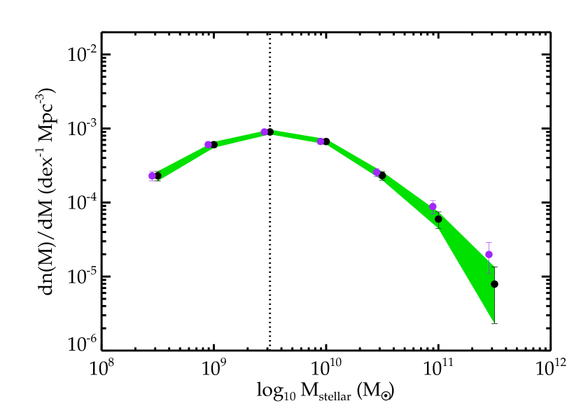
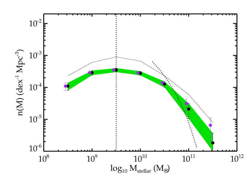
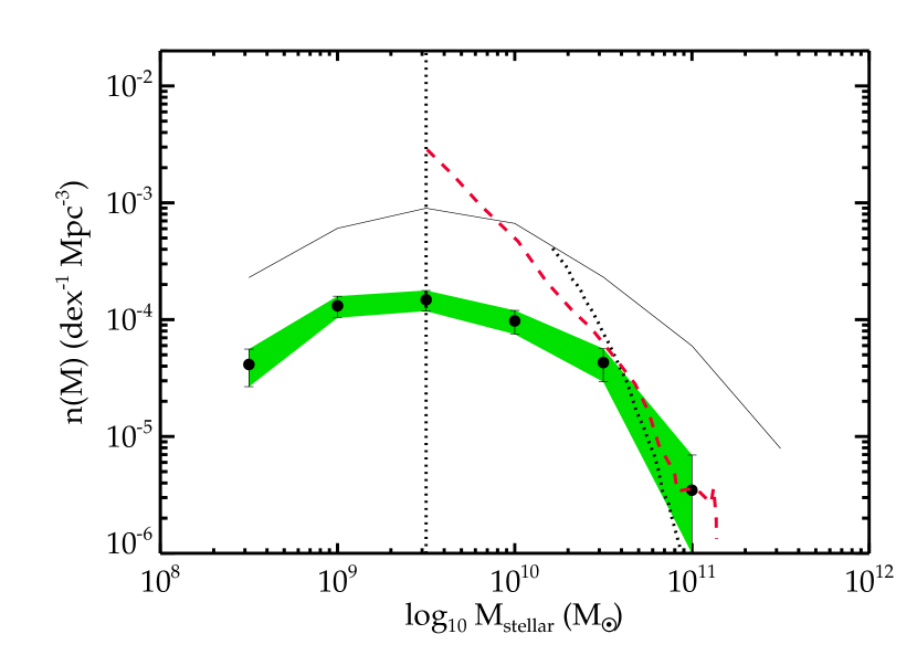
Figure 11.— Stellar Mass Function of B-drops (top panel), V-drops (middle panel), and $i^{\prime}$-drops (bottom panel) with $M_{1500}<-20$. The green swath and associated solid black data points corresponds to the mass function determined from a large sample of dropouts in GOODS-S and GOODS-N. As discussed in §5.1, stellar masses are determined for individual galaxies by fitting the data against CB07 population synthesis models. This plot is constructed from models with exponentially-decaying star formation histories with $\tau$=100 Myr, solar metallicity, and a Salpeter IMF. The purple datapoints (slightly offset from the central mass bin for clarity) correspond to the densities inferred if 24$\mu$m-detected sources are included. The vertical dotted lines represent the mass limit above which the inferred masses are reliable for individual galaxies. The black dotted lines overlaid on the $V$- and $i^{\prime}$-dropout mass functions (upper right and bottom panels) correspond to the stellar mass function estimated in McLure et al. (2008) by multiplying the luminosity function by the average M/L ratio of the dropout population. The red dashed line overlaid on the $i^{\prime}$-drop sample (bottom panel) corresponds to the predictions of the $z\simeq 6$ stellar mass function from the cosmological SPH simulations presented in Nagamine et al. (2008). The black solid curves overlaid in the upper right and bottom panel show the mass function determined in the B-drop sample (upper left panel).

The resulting mass functions are shown in Figure 11. Also shown on the plot (purple datapoints) are the inferred densities if we include sources detected at 24$\mu$m in the mass function analysis. As expected, the 24$\mu$m detections slightly increase the number densities of the B and V-drops in the most massive bins, but generally do not increase them by more than the Poisson uncertainties in that bin. As discussed in §4.2, the inferred stellar mass uncertainties for individual galaxies become considerable for fainter sources with masses $\mathrel{\hbox to0.0pt{\lower 4.0pt\hbox{\hskip 1.0pt$\sim$}\hss}\raise 1.0pt\hbox{$<$}}10^{9.5}$ M_⊙. Although the average properties of sources less massive than this limit are reliable, we nevertheless choose to focus our analysis on the more robustly determined objects contained in bins 10^9.5 M_⊙ and above.

The number densities derived here agree reasonably well with previous measurements. We plot the recent McLure et al. (2008) estimate of the $z\simeq 5$ and 6 LBG stellar mass functions over our curves in Figure 11 (after adjusting their masses to be consistent with a Salpeter IMF). In spite of their approximate way of determining the stellar mass function (the McLure et al. mass function is derived by scaling the luminosity function by the average stellar mass to light ratio), the two estimates agree to within a factor of 2 over the mass range probed, with our determination predicting a larger density of the most massive galaxies. The results also are in reasonable agreement with the massive end of the stellar mass function determined from the cosmological SPH simulations discussed in Nagamine et al. (2008). The observed mass function becomes shallower than the model predictions at $\mathrel{\hbox to0.0pt{\lower 4.0pt\hbox{\hskip 1.0pt$\sim$}\hss}\raise 1.0pt\hbox{$<$}}10^{10.0}$ M_⊙. This may be due, in part, to observational incompleteness at low mass limits. However a similar “knee” in the galaxy mass function is seen in the Drory et al. (2005) data suggesting that the simulations may be underpredicting low-mass galaxies, as suggested by Nagamine et al. (2008).

In contrast to the weakly evolving mass function at $z\mathrel{\hbox to0.0pt{\lower 4.0pt\hbox{\hskip 1.0pt$\sim$}\hss}\raise 1.0pt\hbox{$<$}}1$, the increase in stellar mass between $z\simeq 6$ and $4$ occurs over the entire stellar mass range considered. Between $z\simeq 6$ and $z\simeq 4$, we find a factor of 5-6 increase in density for the bins ranging between 10^9.5 and 10^10.5 M_⊙. There is some evidence that the number density grows more rapidly for the most massive galaxies. While the uncertainties are significant, the mass functions suggest that the number density in the bin centered at 10¹¹ M_⊙ increases by a factor of 17 between $z=6$ and $z=4$, nearly three times greater than the growth in less massive bins. It seems likely that we are witnessing a formative period of massive galaxy formation.

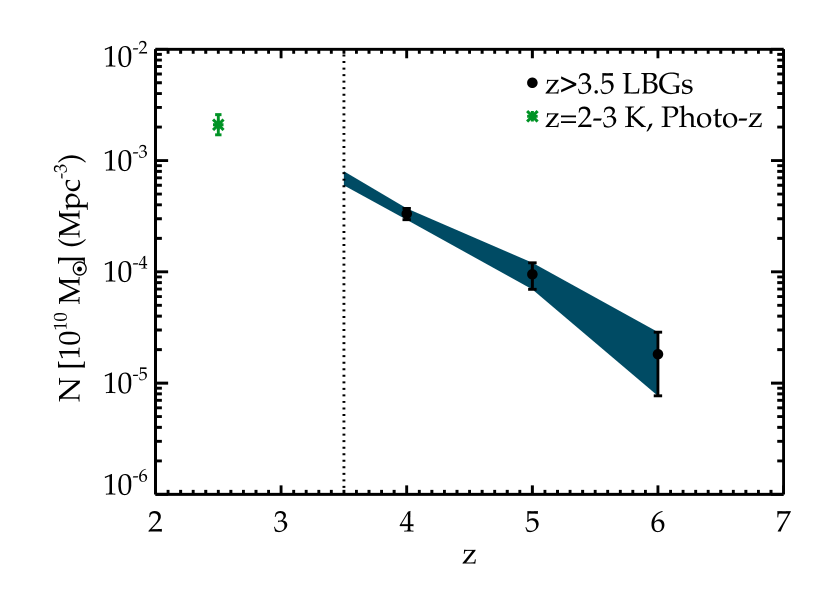
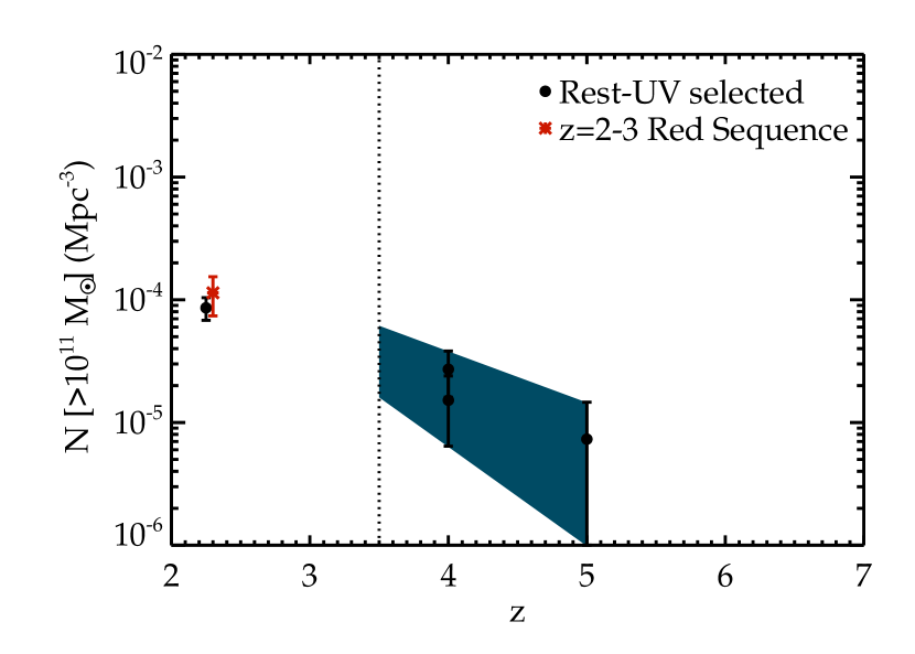
Figure 12.— Evolving number density of massive galaxies at high redshift. Top: Solid black circles (and associated blue swath) show the evolution in the number density of actively forming galaxies more massive than 10¹⁰ M_⊙ derived in this paper. The green asterisk correspond to the total number density of galaxies more massive than 10¹⁰ M_⊙ at $z=2.5$ identified in a K_s-band selected survey (Drory et al., 2005). The vertical dotted line demarcates the redshift range covered in this paper. Bottom: Same as top panel but for galaxies more massive than 10¹¹ M_⊙. The black circles give the number density of rest-UV selected galaxies more massive than 10¹¹ M_⊙; the upper datapoint at $z=4$ corresponds to the number density inferred if the B-drops with 24$\mu$m detections are truly at high redshift. The red asterisk shows the number density of galaxies more massive than 10¹¹ M_⊙ that are quiescent at $z=2.3$ (Kriek et al., 2008).

We finally turn to whether the observed number densities of massive LBGs at $z\mathrel{\hbox to0.0pt{\lower 4.0pt\hbox{\hskip 1.0pt$\sim$}\hss}\raise 1.0pt\hbox{$>$}}2$ can account for a significant component of the largely quiescent population of DRGs at $z\simeq 2$. At $z\mathrel{\hbox to0.0pt{\lower 4.0pt\hbox{\hskip 1.0pt$\sim$}\hss}\raise 1.0pt\hbox{$>$}}4$, we find that the number density of dropouts with stellar mass greater than 10¹¹ M_⊙ (excluding MIPS-detected sources) is $\simeq 2\times 10^{-5}$ Mpc^-3 (Figure 12). We find no overlap between these sources and the massive, sub-mm detected objects recently discovered in GOODS-N (Daddi et al., 2008). If these massive LBGs become quiescent on a timescale of less than 1 Gyr, then we would expect them to appear as red galaxies with little star formation at $z\simeq 2$. Indeed if we evolve the colors and rest-UV luminosities of these massive LBGs forward in time to $z\simeq 2$ assuming the simple exponential decay models considered in §6, we derive colors and optical apparent magnitudes that are consistent with the observed properties of DRGs (van Dokkum et al., 2006). Comparing the observed density of massive LBGs at $z\mathrel{\hbox to0.0pt{\lower 4.0pt\hbox{\hskip 1.0pt$\sim$}\hss}\raise 1.0pt\hbox{$>$}}4$ to the number density of quiescent 10¹¹ M_⊙ systems at $z\simeq 2-3$ (1.1$\times$10^-4 Mpc^-3, Kriek et al. 2008) indicates that at least $\simeq 20$% of the $z\simeq 2-3$ population of quiescent 10¹¹ M_⊙ galaxies formed a large fraction of their stellar mass at $z\mathrel{\hbox to0.0pt{\lower 4.0pt\hbox{\hskip 1.0pt$\sim$}\hss}\raise 1.0pt\hbox{$>$}}3.5$.

Given the expectation that dust-enshrouded “bursts” of star formation seen in the sub-mm are largely responsible for assembling massive galaxies by $z\simeq 2-3$ (Cimatti et al., 2004; McCarthy et al., 2004), it is interesting to extend our estimates of the number density of massive LBGs down to $z\simeq 2$ in order to compute the total fraction of massive galaxies that were formed through objects present in rest-UV selected samples. Shapley et al. (2005) estimate that the number density of UV luminous galaxies with masses in excess of 10¹¹ M_⊙ at $z\simeq 2$ is $\simeq$10^-4 Mpc^-3. We make our own estimate by constructing a sample of rest-UV selected ($z^{\prime}_{850}\mathrel{\hbox to0.0pt{\lower 4.0pt\hbox{\hskip 1.0pt$\sim$}\hss}\raise 1.0pt\hbox{$<$}}26.5$) galaxies in GOODS-S with photometric redshfits between $z=2$ and 2.4 using redshifts and photometry from the GOODS-MUSIC $z^{\prime}_{850}$-band selected catalog (Grazian et al., 2006). We follow the same procedures described earlier for computing stellar masses, completeness as a function of magnitude, and effective volumes. The derived number densities are corrected for incompleteness (the sample is roughly 90% complete at $z^{\prime}_{850}=26$), resulting in final number density estimates of $\simeq\rm{9}\times\rm{10^{-5}}$ Mpc^-3, very close to the measurement from Shapley et al. (2005). These densities suggest that at $z\simeq 2$, the number density of UV-bright massive galaxies is roughly comparable to the density of systems that have already become quiescent.

Computing the contribution of rest-UV selected $z\mathrel{\hbox to0.0pt{\lower 4.0pt\hbox{\hskip 1.0pt$\sim$}\hss}\raise 1.0pt\hbox{$>$}}2$ galaxies to the density of quiescent $z\simeq 2$ systems is non-trivial as it depends strongly on the timescale over which star formation is quenched in the LBGs. The shorter the timescale, the larger the implied number density of quiescent objects at $z\simeq 2$. If we assume that massive LBGs join the red sequence over a period of 500 Myr, then we can estimate a quiescent number density by integrating over the growth in UV luminous massive galaxies over $2\mathrel{\hbox to0.0pt{\lower 4.0pt\hbox{\hskip 1.0pt$\sim$}\hss}\raise 1.0pt\hbox{$<$}}z\mathrel{\hbox to0.0pt{\lower 4.0pt\hbox{\hskip 1.0pt$\sim$}\hss}\raise 1.0pt\hbox{$<$}}6$ (Figure 12). Following this approach, we find that rest-UV selected galaxies would produce a quiescent galaxy density of 7$\times$10^-5 Mpc^-3 by $z\simeq 2.5$, increasing to 2$\times$10^-4 Mpc^-3 at $z\simeq 2$. If the quenching timescale is longer (i.e., 1 Gyr), then the implied quiescent number density decreases to $\simeq 5\times 10^{-5}$ Mpc^-3 at $z\simeq 2$. Hence, these simple assumptions suggest that star formation in rest-UV selected $z\mathrel{\hbox to0.0pt{\lower 4.0pt\hbox{\hskip 1.0pt$\sim$}\hss}\raise 1.0pt\hbox{$>$}}2$ galaxies accounts for the assembly of at least 50% of the total quiescent population of massive galaxies at $z\simeq 2$.

It thus appears reasonable that a significant fraction of the passively-evolving subset of $z\simeq 2-3$ galaxies with 10¹¹ M_⊙ assembled their mass in UV luminous star formation episodes at higher redshifts. While it is possible that these rest-UV selected galaxies would be detectable in deeper sub-mm observations, or alternatively that these galaxies may have undergone short-duration sub-mm luminous bursts of star formation in their past, these results appear to indicate that the ultra-luminous sub-mm galaxies such as those presented in Capak et al. (2008) and Daddi et al. (2008) do not necessarily provide the only route toward assembling massive, quiescent galaxies by $z\simeq 2$. Constructing a complete sample of the precursors of this massive population of red galaxies must include both rest-UV and sub-mm samples.

8. Stellar Mass Densities at $z\simeq 4,5,\rm{and}6$

We now estimate the stellar mass densities implied by our dropout samples. By integrating the mass functions presented in Figure 11, we compute the stellar mass density brightward of the adopted rest-UV magnitude limit (taken to be M₁₅₀₀=$-$20 for each of the dropout samples). This absolute magnitude limit corresponds to apparent magnitude limits of $i^{\prime}_{775}\simeq 26.0$ for the B-drops, z${}_{850}\simeq 26.4$ for the V-drops, and z${}_{850}\simeq 26.7$ for the $i^{\prime}$-drops. Using the $\tau$=100(300) Myr exponential decay models, we obtain 1.1(1.4)$\times$10⁷ M_⊙ Mpc^-3, 3.7(4.9)$\times$10⁶ M_⊙ Mpc^-3, and 1.6(2.3)$\times$10⁶ M_⊙ Mpc^-3 for the B, V, and $i^{\prime}$-drops, respectively (Figure 13). Including all MIPS-detected dropouts sources increases the derived mass densities to 1.6(1.9) $\times$10⁷ M_⊙ Mpc^-3 for the B-drops and 4.7(6.2)$\times$10⁶ M_⊙ Mpc^-3 for the V-drops with the $\tau$=100(300) Myr star formation history. The range of mass densities quoted above are consistent with our previous measurements at $z\simeq 5$ (5$\times$10⁶ M_⊙ Mpc^-3, Stark et al. 2007) and $z\simeq 6$ (2.5$\times$10⁶ M_⊙ Mpc^-3, Eyles et al. 2007).

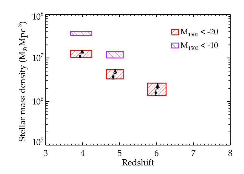
Figure 13.— Stellar mass density of B, V, and $i^{\prime}$-drops. The red rectangles demarcate the stellar mass densities derived from our dropout sample with an adopted magnitude limit of M${}_{1500}=-20$. The circles(triangles) denote mass densities and associated Poisson error determined using CB07 models with an exponentially-declining star formation history with a decay factor of $\tau$=100(300) Myr. See Figure 11 caption and §5.1 for further discussion of the assumptions used in deriving the stellar masses. Purple squares demarcate rough estimates of the total stellar mass density of galaxies brighter than M${}_{1500}=-10$. These values are determined by extrapolating the average relationship between stellar mass and M₁₅₀₀ (Figure 9) to luminosities below the detection limits of the GOODS dataset.

As the total stellar mass density of galaxies at high redshift provides a unique constraint on the past star formation history of the universe, it is of interest to estimate the contribution from galaxies that are fainter than the adopted rest-UV absolute magnitude limit of M₁₅₀₀=-20. For the B and V-drop samples, this magnitude limit is brighter than allowed by the S/N limits of the data (see vertical lines in Figure 9). If we compute the mass density of the B-drop sample including all sources brighter than the 5$\sigma$ limit of M${}_{1500}\simeq-19.1$, we derive a mass density of 1.7(2.1)$\times$10⁷ M_⊙ Mpc^-3. Likewise, integrating the stellar mass function of the V-drop sample including all sources brighter than the 5$\sigma$ limit of M${}_{1500}\simeq-19.5$, we find a mass density of 4.4(5.9)$\times$10⁶ M_⊙ Mpc^-3. Both estimates exclude the contribution of MIPS-detected sources.

In order to constrain the mass density of the population even fainter than these limits, we need to know the average stellar mass to UV luminosity ratio for galaxies below our detection thresholds. We can estimate this by extrapolating the trends present in the M_⋆-M₁₅₀₀ relation of Figure 9. Fitting a linear model to the observed trend for our B-drop sample, we find the following relation: $\overline{\rm{log_{10}M_{\star}}}=-0.26-0.47(\rm{M_{1500}})$. By extrapolating this function to fainter magnitudes and integrating the observed UV luminosity function (Bouwens et al., 2007) to determine the number density of galaxies at each M₁₅₀₀, we can compute a rough estimate the contribution of typical faint UV sources to the total stellar mass density.

Following this approach, we find that the entire population of typical faint B-drops (e.g., those with average stellar masses in the magnitude range $-19\mathrel{\hbox to0.0pt{\lower 4.0pt\hbox{\hskip 1.0pt$\sim$}\hss}\raise 1.0pt\hbox{$<$}}\rm{M_{1500}}\mathrel{\hbox to0.0pt{\lower 4.0pt\hbox{\hskip 1.0pt$\sim$}\hss}\raise 1.0pt\hbox{$<$}}-10$) comprises $\simeq 49$% of the total stellar mass density. This increases the total stellar mass density in B-drops to $\simeq\rm{3.3(4.1)}\times$10⁷ M_⊙ Mpc^-3 for the $\tau$=100(300) Myr exponential decay models. Applying the same procedure to the V-drops (assuming the same relationship between stellar mass and M₁₅₀₀ holds at $z\simeq 5$), we derive total stellar mass densities of 1.0(1.4)$\times$10⁷ M_⊙ Mpc^-3 for sources brighter than M₁₅₀₀=-10. We refrain from making a similar extrapolation for the $i^{\prime}$-drops given the larger uncertainties in this population’s M_⋆-M₁₅₀₀ relation.

9. Summary

We have studied the growth of galaxies over $4\mathrel{\hbox to0.0pt{\lower 4.0pt\hbox{\hskip 1.0pt$\sim$}\hss}\raise 1.0pt\hbox{$<$}}z\mathrel{\hbox to0.0pt{\lower 4.0pt\hbox{\hskip 1.0pt$\sim$}\hss}\raise 1.0pt\hbox{$<$}}6$ with the goal of improving our understanding of galaxy evolution in the first 2 billion years of cosmic history. Using the deep HST data available in the two GOODS fields, we compiled samples of 2819 B-dropouts, 615 V-dropouts, and 166 $i^{\prime}$-dropouts. The superior quality of the multiwavelength data in GOODS (including optical data from HST spanning four filters, near-infrared data from the VLT and Subaru, and mid-infrared data from Spitzer) greatly helps identify foreground galaxies and stars which lurk in Lyman break dropout samples. Great care was taken to identify and remove these objects from our sample, using HST morphologies to excise point sources likely to be bright stellar contaminants and broadband SEDs spanning from the optical to the infrared to remove low-redshift galaxies.

Our final high-redshift sample consists of 2443 B-dropouts, 506 V-dropouts, and 137 $i^{\prime}$-dropouts. From this sample of galaxies, we constructed sub-samples of dropouts which are sufficiently unblended with nearby foreground objects in the deep Spitzer data to allow accurate photometry. In general, this corresponds to $\mathrel{\hbox to0.0pt{\lower 4.0pt\hbox{\hskip 1.0pt$\sim$}\hss}\raise 1.0pt\hbox{$>$}}35$% of the total samples. We used the CB07 population synthesis models to estimate stellar masses and ages for this “Spitzer clean” subset. We compared the inferred properties to those derived from BC03 models, finding general agreement for solar metallicity models when the redshift is above 5. Below this redshift, the mid-IR data begin to probe the rest-frame near-infrared (which is affected by TP-AGB stars), and the CB07 models therefore return masses which are typically 10% lower than those from BC03 models.

Using this large database of stellar masses and rest-UV properties of B, V, and $i^{\prime}$-dropouts, we examine the evolution of star-forming galaxies between $z\simeq 4$ and 6. We summarize our main results below.

1. We find that the typical stellar masses and ages of galaxies of a fixed UV luminosity (uncorrected for dust extinction) do not evolve strongly between $z\simeq 6$, 5, and 4. This argues against the notion that the B-drops are made up of galaxies that have been steadily growing at fixed UV luminosity since $z\simeq 6$. Instead, these data suggest that each successive epoch studied in this survey (e.g., $z\simeq 4$, 5, and 6) is likely dominated by galaxies that have only recently (within the last $\simeq 300$ Myr) emerged at their present luminosity. This is consistent with the observed decline in the UV luminosity function between $z\simeq 4$ and 6 (Bouwens et al., 2007).

2. The evolution in the M_⋆-M₁₅₀₀ relation and the UV luminosity function is potentially difficult to reconcile if the galaxies observed at $z\mathrel{\hbox to0.0pt{\lower 4.0pt\hbox{\hskip 1.0pt$\sim$}\hss}\raise 1.0pt\hbox{$>$}}4$ assembled their stars with a constant star formation rate. In this scenario, the inferred ages of galaxies at one epoch are sufficiently large to violate the required decline in the UV LF and the lack of strong evolution in the M_⋆-M₁₅₀₀. However if lower metallicity templates are adopted, the ages are lowered and the discrepancy reduced. Deeper infrared photometry will be of significant benefit in improving constraints on the inferred stellar populations.

We also considered a steady growth scenario in which star formation is becoming steadily more vigorous with increasing cosmic time between $z\simeq 6$ and $z\simeq 4$, as predicted in the simulations of Finlator et al. (2006). In this case, the inferred ages of the galaxies remain large, but since their precursors are fainter in the past, they don’t violate the observed evolution in the UV LF and M_⋆-M₁₅₀₀ relation. The only problem that potentially stands in the way of this model is that it is inconsistent with the short duty cycles implied by measurements of the clustering of $z\mathrel{\hbox to0.0pt{\lower 4.0pt\hbox{\hskip 1.0pt$\sim$}\hss}\raise 1.0pt\hbox{$>$}}4$ LBGs (Lee et al., 2008). Additional spectroscopy and new multiwavelength imaging in independent fields are required to confirm these clustering measurements.

3. We argue that episodic star formation may provide the best fit to the wide range of observations considered in this paper. In this picture, each epoch is dominated by recently emerged sources, which remain luminous for no more than $\simeq 500$ Myr on average. If the UV luminous periods become more intense with cosmic time between $z\simeq 6$ and 4, then this scenario could explain the evolution of the M_⋆-M₁₅₀₀ relation and the UV LF. If this is the dominant mode of star formation at $z\mathrel{\hbox to0.0pt{\lower 4.0pt\hbox{\hskip 1.0pt$\sim$}\hss}\raise 1.0pt\hbox{$>$}}4$, then there should be a significant population of relatively massive, quiescent sources that are in between star formation episodes. Future efforts at $z\simeq 4$ should help clarify whether this is the case.

4. The stellar mass function of UV luminous sources grows significantly from $z\approx 6$ to $z\approx 4$, typically increasing by more than a factor of six in number density over the entire stellar mass range considered. There is some evidence that the growth in the most massive LBGs (M${}_{\star}\simeq\rm{10^{11\pm 0.5}}$) is a factor of three greater than in less massive systems, implying that this redshift range likely corresponds to the beginning of massive (10¹¹ M_⊙) galaxy formation era.

5. The rapid growth in the assembly of massive galaxies at $z\mathrel{\hbox to0.0pt{\lower 4.0pt\hbox{\hskip 1.0pt$\sim$}\hss}\raise 1.0pt\hbox{$>$}}4$ indicates that at least $\simeq 20$% of the $z\simeq 2-3$ quiescent massive galaxies assembled their stellar mass at $z\mathrel{\hbox to0.0pt{\lower 4.0pt\hbox{\hskip 1.0pt$\sim$}\hss}\raise 1.0pt\hbox{$>$}}3.5$. Fitting the increase in number density of UV luminous, massive galaxies between $z\simeq 6$ and 2, we estimate that it is feasible that more than 50% of quiescent $z\simeq 2-3$ massive galaxies were assembled in higher redshift LBGs. These results imply that the high star formation rate, dust-obscured sub-mm galaxies are not the only route toward assembling quiescent 10¹¹ M_⊙ systems by $z\simeq 2-3$.

6. Using the CB07 models with solar metallicity and a exponentially declining star formation history with a decay factor of $\tau$=100(300) Myr, we derive the stellar mass density of rest-UV selected dropouts brighter than M${}_{1500}=-20$: $\rho_{\star}\simeq 1.1$(1.4)$\times$10⁷ M_⊙ Mpc^-3 at $z\simeq 4$, 3.7(4.9)$\times$10⁶ M_⊙ Mpc^-3 at $z\simeq 5$, and 1.6(2.3) $\times$10⁶ M_⊙ Mpc^-3 at $z\simeq 6$. These measurements are certain to underpredict the total stellar mass density since they do not include the contribution from sources that either do not satisfy are color selection criteria or lie faintward of the absolute magnitude limit. By extrapolating the M_⋆-M₁₅₀₀ relation from Figure 9 to M₁₅₀₀=-10 and integrating the UV luminosity functions of Bouwens et al. (2007), we estimate that the population of faint galaxies may increase the mass density estimates quoted above by a factor of 3-5$\times$.

ACKNOWLEDGMENTS

We thank the referee for a very helpful report and acknowledge useful conversations with Tommaso Treu, Niv Drory, and Masami Ouchi. DPS thanks the Department of Astrophysics at the University of Oxford for its hospitality while much of this work was being conducted and acknowledges financial support from the STFC. RSE acknowledges financial support from the Royal Society. This paper is based on observations made with the NASA/ESA Hubble Space Telescope, obtained from the Data Archive at the Space Telescope Science Institute, which is operated by the Association of Universities for Research in Astronomy, Inc., under NASA contract NAS 5-26555. The HST/ACS observations are associated with proposals #9425 & 9583 (the GOODS public imaging survey).

References

- Arnouts et al. (2001) Arnouts, S., et al. 2001, A&A, 379, 740
- Beckwith et al. (2006) Beckwith, S. V. W., et al. 2006, AJ, 132, 1729
- Benítez (2000) Benítez, N. 2000, ApJ, 536, 571
- Birnboim & Dekel (2003) Birnboim, Y., & Dekel, A. 2003, MNRAS, 345, 349
- Bouwens et al. (2004) Bouwens, R. J., Illingworth, G. D., Blakeslee, J. P., Broadhurst, T. J., & Franx, M. 2004, ApJ, 611, L1
- Bouwens et al. (2006) Bouwens, R. J., Illingworth, G. D., Blakeslee, J. P., & Franx, M. 2006, ApJ, 653, 53
- Bouwens et al. (2007) Bouwens, R. J., Illingworth, G. D., Franx, M., & Ford, H. 2007, ApJ, 670, 928
- Bower et al. (2006) Bower, R. G., Benson, A. J., Malbon, R., Helly, J. C., Frenk, C. S., Baugh, C. M., Cole, S., & Lacey, C. G. 2006, MNRAS, 370, 645
- Bruzual (2007) Bruzual, G. 2007, Proceedings of the IAU Symposium No. 241 ”Stellar populations as building blocks of galaxies”, astro-ph/0703052
- Bruzual & Charlot (2003) Bruzual, G., & Charlot, S. 2003, MNRAS, 344, 1000
- Bundy et al. (2009) Bundy, K., Fukugita, M., Ellis, R. S., Targett, T. T., Belli, S., & Kodama, T. 2009, Submitted to ApJ
- Bunker et al. (2004) Bunker, A. J., Stanway, E. R., Ellis, R. S., & McMahon, R. G. 2004, MNRAS, 355, 374
- Calzetti (1997) Calzetti, D. 1997, AJ, 113, 162
- Capak et al. (2008) Capak, P., et al. 2008, ApJ, 681, L53
- Capak et al. (2004) Capak, P., et al. 2004, AJ, 127, 180
- Chabrier (2003) Chabrier, G. 2003, PASP, 115, 763
- Chapman et al. (2003) Chapman, S. C., Blain, A. W., Ivison, R. J., & Smail, I. R. 2003, Nature, 422, 695
- Chapman et al. (2005) Chapman, S. C., Blain, A. W., Smail, I., & Ivison, R. J. 2005, ApJ, 622, 772
- Cimatti et al. (2004) Cimatti, A., et al. 2004, Nature, 430, 184
- Coe et al. (2006) Coe, D., Benítez, N., Sánchez, S. F., Jee, M., Bouwens, R., & Ford, H. 2006, AJ, 132, 926
- Coleman et al. (1980) Coleman, G. D., Wu, C.-C., & Weedman, D. W. 1980, ApJS, 43, 393
- Daddi et al. (2008) Daddi, E., et al. 2008, accepted in ApJ, arXiv:0810.3108
- Daddi et al. (2007) Daddi, E., et al. 2007, ApJ, 670, 156
- Davé (2008) Davé, R. 2008, MNRAS, 385, 147
- Drory et al. (2005) Drory, N., Salvato, M., Gabasch, A., Bender, R., Hopp, U., Feulner, G., & Pannella, M. 2005, ApJ, 619, L131
- Egami et al. (2005) Egami, E., et al. 2005, ApJ, 618, L5
- Ellis (2008) Ellis, R. S. 2008, Observations of the High Redshift Universe (Saas-Fee Advanced Course 36: Cold Aqueous Planetary Geochemistry with FREZCHEM), 259
- Erb et al. (2006) Erb, D. K., Steidel, C. C., Shapley, A. E., Pettini, M., Reddy, N. A., & Adelberger, K. L. 2006, ApJ, 646, 107
- Eyles et al. (2007) Eyles, L. P., Bunker, A. J., Ellis, R. S., Lacy, M., Stanway, E. R., Stark, D. P., & Chiu, K. 2007, MNRAS, 374, 910
- Eyles et al. (2005) Eyles, L. P., Bunker, A. J., Stanway, E. R., Lacy, M., Ellis, R. S., & Doherty, M. 2005, MNRAS, 364, 443
- Finlator et al. (2007) Finlator, K., Davé, R., & Oppenheimer, B. D. 2007, MNRAS, 376, 1861
- Finlator et al. (2006) Finlator, K., Davé, R., Papovich, C., & Hernquist, L. 2006, ApJ, 639, 672
- Franx et al. (2003) Franx, M., et al. 2003, ApJ, 587, L79
- Giacconi et al. (2002) Giacconi, R., et al. 2002, ApJS, 139, 369
- Giavalisco et al. (2004a) Giavalisco, M., et al. 2004a, ApJ, 600, L103
- Giavalisco et al. (2004b) Giavalisco, M., et al. 2004b, ApJ, 600, L93
- Grazian et al. (2006) Grazian, A., et al. 2006, A&A, 449, 951
- Hopkins & Beacom (2006) Hopkins, A. M., & Beacom, J. F. 2006, ApJ, 651, 142
- Ichikawa et al. (2006) Ichikawa, T., et al. 2006, in Society of Photo-Optical Instrumentation Engineers (SPIE) Conference Series, Vol. 6269, Society of Photo-Optical Instrumentation Engineers (SPIE) Conference Series
- Kereš et al. (2005) Kereš, D., Katz, N., Weinberg, D. H., & Davé, R. 2005, MNRAS, 363, 2
- Kinney et al. (1996) Kinney, A. L., Calzetti, D., Bohlin, R. C., McQuade, K., Storchi-Bergmann, T., & Schmitt, H. R. 1996, ApJ, 467, 38
- Kriek et al. (2008) Kriek, M., van der Wel, A., van Dokkum, P. G., Franx, M., & Illingworth, G. D. 2008, ArXiv e-prints, 804
- Kriek et al. (2006) Kriek, M., et al. 2006, ApJ, 645, 44
- Labbé et al. (2005) Labbé, I., et al. 2005, ApJ, 624, L81
- Lee et al. (2008) Lee, K. ., Giavalisco, M., Conroy, C., Wechsler, R. H., Ferguson, H. C., Somerville, R. S., Dickinson, M. E., & Urry, C. M. 2008, ArXiv e-prints
- Lee et al. (2006) Lee, K.-S., Giavalisco, M., Gnedin, O. Y., Somerville, R. S., Ferguson, H. C., Dickinson, M., & Ouchi, M. 2006, ApJ, 642, 63
- Madau (1995) Madau, P. 1995, ApJ, 441, 18
- Maraston (2005) Maraston, C. 2005, MNRAS, 362, 799
- Marigo & Girardi (2007) Marigo, P., & Girardi, L. 2007, A&A, 469, 239
- McCarthy et al. (2004) McCarthy, P. J., et al. 2004, ApJ, 614, L9
- McLure et al. (2008) McLure, R. J., Cirasuolo, M., Dunlop, J. S., Foucaud, S., & Almaini, O. 2008, ArXiv e-prints, 805
- Meurer et al. (1999) Meurer, G. R., Heckman, T. M., & Calzetti, D. 1999, ApJ, 521, 64
- Nagamine et al. (2008) Nagamine, K., Ouchi, M., Springel, V., & Hernquist, L. 2008, ArXiv e-prints, 802
- Noeske et al. (2007) Noeske, K. G., et al. 2007, ApJ, 660, L47
- Oke & Gunn (1983) Oke, J. B., & Gunn, J. E. 1983, ApJ, 266, 713
- Ouchi et al. (2004) Ouchi, M., et al. 2004, ApJ, 611, 685
- Papovich et al. (2001) Papovich, C., Dickinson, M., & Ferguson, H. C. 2001, ApJ, 559, 620
- Papovich et al. (2006) Papovich, C., et al. 2006, ApJ, 640, 92
- Pirzkal et al. (2005) Pirzkal, N., et al. 2005, ApJ, 622, 319
- Reddy et al. (2006) Reddy, N. A., Steidel, C. C., Fadda, D., Yan, L., Pettini, M., Shapley, A. E., Erb, D. K., & Adelberger, K. L. 2006, ApJ, 644, 792
- Reddy et al. (2008) Reddy, N. A., Steidel, C. C., Pettini, M., Adelberger, K. L., Shapley, A. E., Erb, D. K., & Dickinson, M. 2008, ApJS, 175, 48
- Salpeter (1955) Salpeter, E. E. 1955, ApJ, 121, 161
- Schlegel et al. (1998) Schlegel, D. J., Finkbeiner, D. P., & Davis, M. 1998, ApJ, 500, 525
- Shapley et al. (2001) Shapley, A. E., Steidel, C. C., Adelberger, K. L., Dickinson, M., Giavalisco, M., & Pettini, M. 2001, ApJ, 562, 95
- Shapley et al. (2005) Shapley, A. E., Steidel, C. C., Erb, D. K., Reddy, N. A., Adelberger, K. L., Pettini, M., Barmby, P., & Huang, J. 2005, ApJ, 626, 698
- Smail et al. (1998) Smail, I., Ivison, R. J., Blain, A. W., & Kneib, J.-P. 1998, ApJ, 507, L21
- Stanway et al. (2007) Stanway, E. R., et al. 2007, MNRAS, 376, 727
- Stanway et al. (2003) Stanway, E. R., Bunker, A. J., & McMahon, R. G. 2003, MNRAS, 342, 439
- Stanway et al. (2004) Stanway, E. R., Bunker, A. J., McMahon, R. G., Ellis, R. S., Treu, T., & McCarthy, P. J. 2004, ApJ, 607, 704
- Stanway et al. (2005) Stanway, E. R., McMahon, R. G., & Bunker, A. J. 2005, MNRAS, 359, 1184
- Stark et al. (2007) Stark, D. P., Bunker, A. J., Ellis, R. S., Eyles, L. P., & Lacy, M. 2007, ApJ, 659, 84
- Steidel et al. (1999) Steidel, C. C., Adelberger, K. L., Giavalisco, M., Dickinson, M., & Pettini, M. 1999, ApJ, 519, 1
- Steidel et al. (1996) Steidel, C. C., Giavalisco, M., Pettini, M., Dickinson, M., & Adelberger, K. L. 1996, ApJ, 462, L17
- van Dokkum (2008) van Dokkum, P. G. 2008, ApJ, 674, 29
- van Dokkum et al. (2004) van Dokkum, P. G., et al. 2004, ApJ, 611, 703
- van Dokkum et al. (2006) van Dokkum, P. G., et al. 2006, ApJ, 638, L59
- Vanzella et al. (2002) Vanzella, E., et al. 2002, A&A, 396, 847
- Vanzella et al. (2008) Vanzella, E., et al. 2008, A&A, 478, 83
- Vanzella et al. (2005) Vanzella, E., et al. 2005, A&A, 434, 53
- Vanzella et al. (2009) Vanzella, E., et al. 2009, Accepted for Publication in ApJ, arXiv:0901.4364
- Verma et al. (2007) Verma, A., Lehnert, M. D., Förster Schreiber, N. M., Bremer, M. N., & Douglas, L. 2007, MNRAS, 377, 1024
- Webb et al. (2006) Webb, T. M. A., et al. 2006, ApJ, 636, L17
- Westera et al. (2002) Westera, P., Lejeune, T., Buser, R., Cuisinier, F., & Bruzual, G. 2002, A&A, 381, 524
- Wilkins et al. (2008) Wilkins, S. M., Trentham, N., & Hopkins, A. M. 2008, MNRAS, 385, 687
- Williams et al. (1996) Williams, R. E., et al. 1996, AJ, 112, 1335
- Yan et al. (2005) Yan, H., et al. 2005, ApJ, 634, 109
- Yoshida et al. (2006) Yoshida, M., et al. 2006, ApJ, 653, 988