A Redshift-Magnitude Relation for Non-Uniform Pressure Universes

Abstract

A redshift-magnitude relation for the two exact non-uniform pressure spherically symmetric Stephani universes is presented. The Kristian-Sachs method expanding the relativistic quantities in series is used, but only first order terms in redshift $z$ are considered. The numerical results are given both for centrally placed and non-centrally placed observers. In the former case the redshift-magnitude relation does not depend on the direction in the sky and the Friedman limit can be easily performed. It appears that the effect of spatial dependence of pressure is similar to the effect of the deceleration parameter in Friedman models. In the latter case the angular dependence of the relation is important. This may serve as another possible explanation of the noncompatibility of the theoretical curve of the redshift-magnitude relation with observations for large redshift objects in the Friedman universe. On the other hand comparing the magnitudes of equal redshifts objects in different directions in the sky one can test the reliability of these models.

Journal Reference: The Astrophysical Journal 447, 43 (1995).

1 INTRODUCTION

Inhomogeneous models of the Universe have gradually become more popular among cosmologists. Although we know quite a lot of different inhomogeneous solutions (e.g. Kramer et al. 1980, Krasiński 1993) the most famous and strongly investigated models of this general class have been the spherically symmetric dust Tolman universes (Tolman 1934, Bondi 1947, Bonnor 1974). Their properties have been studied quite thoroughly by Hellaby and Lake (1984, 1985), Hellaby (1987, 1988) and the observational relations for them were studied by Goicoechea and Martin-Mirones (1986), Moffat and Tatarski (1992).

Recently, we have considered the global properties of the spherically symmetric Stephani universes (Da̧browski 1993). A couple of exact inhomogeneous solutions have been found and the question arises how far from the real Universe these solutions can be. The purpose of this paper is to give the observational relations that could enable us to compare these solutions with astronomical observations of galaxies and quasars.

Generally, in inhomogeneous models the density and (or) pressure depend on spatial coordinates. The density in the Tolman models is non-uniform. By this we mean that it depends on both the time and the radial coordinate. On the other hand the pressure is uniform and it only depends on the time coordinate. In the Stephani models it is quite different - the density is uniform and the pressure is non-uniform. Although it seems to be easier to think about non-uniform density in the Universe, the non-uniform pressure could still have some motivation in inflationary cosmology, at least in the very early stages of the Universe when the vacuum pressure plays an important role (Vilenkin 1985, Weinberg 1989, Linde 1994). The Stephani models have also been studied in the context of thermodynamics by Sussman (1994), Quevedo and Sussman (1994a,b).

Some other possibilities of admitting inhomogeneities in the Universe have been studied, among others, by Roeder (1975), Dyer (1979), Partovi and Mashhoon (1984). Some observational quantities for these models have also been found.

In this paper we shortly comment on the Stephani models in Section 2. In Section 3 we present a formula for the redshift in Model I (MI) and Model II (MII) which have been fully considered in the earlier paper (Da̧browski 1993). In Section 4 we use the Kristian-Sachs method (Kristian and Sachs 1966) to derive the redshift-magnitude relations for MI and MII. In Section 5 we present numerical results for the redshift-magnitude relation both for centrally and non-centrally placed observers. In the Appendix A we write down the components of the null tangent vector to zero geodesic equations and solve them in a couple of cases. In the Appendix B we present a redshift-magnitude relation for a radial ray in the general spherically symmetric Stephani universe.

2 The Models

The spherically symmetric Stephani metric is given by (Krasiński 1983, Da̧browski 1993)

$$ds^{2}~{}=~{}-~{}D^{2}c^{2}dt^{2}~{}+~{}\frac{R^{2}}{V^{2}}\left[dr^{2}~{}+~{}r^{2}\left(d\theta^{2}~{}+~{}\sin^{2}{\theta}d\varphi^{2}\right)\right]~{},$$ (2-1)

where

$$V(t,r) = 1+\frac{1}{4}kr^{2}~{},$$ (2-2)

$$D(t,r) = F\frac{R}{V}\left(\frac{V}{R}\right)^{\cdot}~{},$$ (2-3)

$$k(t) = \left(C^{2}(t)~{}-~{}\frac{1}{c^{2}F^{2}(t)}\right)~{}R^{2}(t)~{},$$ (2-4)

and $(\ldots)^{\cdot}~{}\equiv~{}\frac{\partial}{\partial t}$. In (2.1)-(2.4) we have chosen the following units: the time t is taken in sMpc/km, the function $R(t)$ (generalized scale factor) is taken in megaparsecs or kilometers, the function $F(t)$ is in seconds, the dimension of $C(t)$ is $km^{-1}$, $c=3\cdot 10^{5}$ km/s is the velocity of light and all the other functions $r,\theta,\phi,D(t,r),V(t,r),k(t)$ are dimensionless. The mass density and pressure are given by

$$\frac{8\pi G}{c^{2}}\rho(t) = 3C^{2}(t)~{},$$ (2-5)

$$\frac{8\pi G}{c^{4}}p(t) = -~{}3C^{2}(t)~{}+~{}2C\dot{C}\frac{\left(\frac{V}{R}\right)}{\left(\frac{V}{R}\right)^{\cdot}}~{},$$ (2-6)

where $G$ is the gravitational constant. This means that the density is uniform while the pressure is non-uniform throughout the Stephani universe. The four-velocity of matter has only one nonvanishing component

$$u_{t}~{}=~{}-~{}cD~{},$$ (2-7)

and the only nonvanishing component of the acceleration is

$$\dot{u}_{r}~{}=~{}c\frac{D_{,r}}{D}~{},$$ (2-8)

and $(\ldots)_{,r}~{}\equiv~{}\frac{\partial}{\partial r}$ .

In this paper we will be considering only two subcases of the model (2.1), which possess the flat Friedman limit, so the comparison with the isotropic data seems to be very easy for them. We will be called these subcases Model I (MI) and Model II (MII), respectively. These models admit a Friedman-like time coordinate

$$d\tau~{}=~{}-~{}\int F\frac{\dot{R}}{R}dt~{},$$ (2-9)

in which the expansion scalar is simply $\Theta~{}=~{}3H~{}=~{}3R_{,\tau}/R$. For the Model I we have $C(t)=AR(t)$ with $A=$const. (Da̧browski 1993) and

$$k(\tau) = -~{}4\frac{a}{c^{2}}R(\tau)~{},$$ (2-10)

$$R(\tau) = a\tau^{2}~{}+~{}b\tau~{}+~{}d~{},$$ (2-11)

$$V(\tau,r) = 1~{}-~{}\frac{a}{c^{2}}\left(a\tau^{2}~{}+~{}b\tau~{}+~{}d\right)r^{2}~{},$$ (2-12)

$$\Delta \equiv 4ad~{}-~{}b^{2}~{}+~{}1~{}=~{}0~{},$$ (2-13)

with a, b, d = const. and for the cosmic time $\tau$ taken in sMpc/km we have: [a] = $km^{2}/(s^{2}Mpc)$, [b] = km/s and [c] = Mpc. For the Model II we have (Wesson and Ponce de Leon 1989, Da̧browski 1993)

$$k(\tau) = -~{}\frac{\alpha\beta}{c^{2}}R(\tau)~{},$$ (2-14)

$$R(\tau) = \beta\tau^{\frac{2}{3}}~{},$$ (2-15)

$$V(\tau,r) = 1~{}-~{}\frac{1}{4c^{2}}\alpha\beta^{2}\tau^{\frac{2}{3}}r^{2}~{},$$ (2-16)

with $\alpha$, $\beta$ = const. with $[\alpha]$ = $(s/km)^{\frac{2}{3}}Mpc^{-\frac{4}{3}}$ and $[\beta]$ = $(km/s)^{\frac{2}{3}}Mpc^{\frac{1}{3}}$. Both models possess the Friedman limit; ($a\rightarrow 0$ for MI and $\alpha\rightarrow 0$ for MII). The common point between MI and MII is that for them $\left(\frac{k}{R}\right)_{,\tau}=0$, where $(\ldots)_{,\tau}~{}\equiv~{}\frac{\partial}{\partial\tau}$ (cf. Appendix A) and $D~{}=~{}1/V$ (cf.(2.3)). The four-velocity and the acceleration (2.7)-(2.8) read as

$$u_{\tau} = -~{}c\frac{1}{V}~{},$$ (2-17)

$$\dot{u}_{r} = -~{}c\frac{V_{,r}}{V}~{}.$$ (2-18)

The components of the vector tangent to zero geodesic are (see Appendix A)

$$k^{\tau} = \frac{V^{2}}{R}~{},$$ (2-19)

$$k^{r} = \pm\frac{V^{2}}{R^{2}}\sqrt{1~{}-~{}\frac{h^{2}}{r^{2}}}~{},$$ (2-20)

$$k^{\theta} = 0~{},$$ (2-21)

$$k^{\varphi} = h\frac{V^{2}}{R^{2}r^{2}}~{},$$ (2-22)

where $h$ = const., and the plus sign in (2.20) applies to a ray moving away from the centre, while the minus sign applies to a ray moving towards the centre. The acceleration scalar for MI and MII respectively is

$$\dot{u}~{}\equiv\left(\dot{u}_{a}\dot{u}^{a}\right)^{\frac{1}{2}}~{}=~{}\frac{V_{,r}}{R}~{}=~{}\left\{\begin{array}[]{l}-~{}2\frac{a}{c^{2}}r,\\ -~{}\frac{1}{2}\alpha\beta r,\end{array}\right.\$$ (2-23)

and it does not depend on the time coordinate at all. Also, it means that the further away from the center $r=0$ is an observer, the larger acceleration he subjects.

3 The Redshift

For any cosmological model the redshift is given by (Ehlers 1961, Ellis and MacCallum 1970)

$$1~{}+~{}z~{}=~{}\frac{\left(u_{a}k^{a}\right)_{O}}{\left(u_{a}k^{a}\right)_{G}}~{},$$ (3-1)

where index ’O’ means that the quantities should be taken at the observer position, while index ’G’ means that the quantities should be taken at the galaxy position. According to (3.1), (2.7) and (2.19)-(2.22) we have for MI and MII respectively

$$1~{}+~{}z~{}=\left\{\begin{array}[]{l}\frac{\left[\frac{1~{}-~{}\frac{a}{c^{2}}(a\tau^{2}~{}+~{}b\tau~{}+~{}d)r^{2}}{a\tau^{2}~{}+~{}b\tau~{}+~{}d}\right]_{O}}{\left[\frac{1~{}-~{}\frac{a}{c^{2}}(a\tau^{2}~{}+~{}b\tau~{}+~{}d)r^{2}}{a\tau^{2}~{}+~{}b\tau~{}+~{}d}\right]_{G}},\\ \frac{\left[\frac{1~{}-~{}\frac{1}{4}\alpha\beta^{2}\tau^{\frac{2}{3}}r^{2}}{\beta\tau^{\frac{2}{3}}}\right]_{O}}{\left[\frac{1~{}-~{}\frac{1}{4}\alpha\beta^{2}\tau^{\frac{2}{3}}r^{2}}{\beta\tau^{\frac{2}{3}}}\right]_{G}}.\end{array}\right.\$$ (3-2)

For corresponding flat Friedman limits

$$1~{}+~{}z~{}=~{}\left\{\begin{array}[]{l}\frac{(b\tau~{}+~{}d)_{G}}{(b\tau~{}+~{}d)_{O}},\\ \frac{(\tau^{\frac{2}{3}})_{G}}{(\tau^{\frac{2}{3}})_{O}}.\end{array}\right.\$$ (3-3)

The first limit corresponds to the exotic equation of state model $p~{}=~{}-~{}\frac{1}{3}\rho$ (Vilenkin 1985, Da̧browski and Stelmach 1989) and the second corresponds to the dust model $p~{}=~{}0$.

From (3.2) one can easily notice that, for instance for the model MII, if the observer is at the centre of symmetry $r~{}=~{}0$ the redshift of a given galaxy lying away from the centre is greater than in corresponding Friedman model (3.3). On the other hand, if it is a galaxy at the centre $r~{}=~{}0$ and the observer is away from it, the redshift of the galaxy measured by the observer is smaller than in the corresponding Friedman model (3.3).

4 The Redshift-Magnitude Relation

The standard procedure in order to obtain the redshift-magnitude relation in power series around the observer position and time is based on the formalism given by Kristian and Sachs (1966) and Ellis and MacCallum (1970). In this paper we assume the signature convention $(-,+,+,+)$ used by Ellis and MacCallum. The redshift-magnitude formula is given by

$$m_{bol}=M-5\log_{10}{\left(u_{a;b}K^{a}K^{b}\right)_{O}}+5\log_{10}{cz}$$

$$+\frac{5}{2}\left(\log_{10}{e}\right)\left\{\left(4-\frac{u_{a;bc}K^{a}K^{b}K^{c}}{\left(u_{a;b}K^{a}K^{b}\right)^{2}}\right)z+{\bf O}\left(z^{2}\right)\right\}_{O}~{},$$ (4-1)

where

$$u_{a;b} = \frac{1}{3}\Theta h_{ab}-\dot{u}_{a}u_{b}~{},$$ (4-2)

$$h_{ab} \equiv g_{ab}+u_{a}u_{b}~{},$$ (4-3)

$$K^{a} \equiv \frac{k^{a}}{u_{b}k^{b}}~{},$$ (4-4)

$$u_{a}u^{a} = -1~{}.$$ (4-5)

Here $m_{bol}$ is the bolometric apparent magnitude, $M$ - absolute magnitude, $\Theta$ - the expansion scalar, $\dot{u}_{a}$ - the acceleration vector, $u_{a}$ - the four-velocity of matter, $k^{a}$ - null vector tangent to the zero geodesic that connects galaxy and observer, $h_{ab}$ - the operator that projects vectors onto spacelike hypersurfaces ($h_{ab}u^{b}=0$, $K_{a}K^{b}=0$, $\dot{u}_{a}u^{a}=0$, $u_{a}K^{a}=1$). The projection of $K^{a}$ onto the spatial hypersurfaces ortogonal to $u_{a}$ - a spatial unit vector pointing in the observer direction of the source is

$$n^{a}=-u^{a}-K^{a},$$ (4-6)

and

$$n^{a}n_{a}=1.$$ (4-7)

From (4.2)-(4.4) we have

$$u_{a;bc}=\frac{1}{3}\Theta_{,c}h_{ab}+\frac{1}{9}\Theta^{2}\left(h_{ac}u_{b}+h_{bc}u_{a}\right)-\dot{u}_{a;c}u_{b}$$

$$-\frac{1}{3}\Theta\left(\dot{u}_{a}u_{b}u_{c}+u_{a}\dot{u}_{b}u_{c}\right)-\frac{1}{3}\Theta\dot{u}_{a}h_{bc}+\dot{u}_{a}\dot{u}_{b}u_{c},$$ (4-8)

In order to calculate (4.1) we should use (4.3) and put it into (4.2) and (4.8) i.e.

$$u_{a;b}K^{a}K^{b} = \frac{1}{3}\Theta-\dot{u}_{a}K^{a},$$ (4-9)

$$u_{a;bc}K^{a}K^{b}K^{c} = \frac{1}{3}\Theta_{,c}K^{c}+\frac{2}{9}\Theta^{2}-\Theta\dot{u}_{a}K^{a}-\dot{u}_{a;c}K^{a}K^{c}+\dot{u}_{a}\dot{u}_{b}u_{c},$$ (4-10)

what according to (2.7) and (2.8) gives

$$u_{a;b}K^{a}K^{b} = \frac{1}{3}\Theta+c\frac{D_{,r}}{D^{2}}\frac{k^{r}}{k^{t}},$$ (4-11)

$$u_{a;bc}K^{a}K^{b}K^{c} = -\frac{1}{3}\frac{\dot{\Theta}}{D}+\frac{2}{9}\Theta^{2}+\frac{c}{D^{2}}\frac{k^{r}}{k^{t}}\times$$ (4-12)

$$\left\{4\Theta D_{,r}-\left(\frac{D_{,r}}{D}\right)_{,t}-c\left[\left(\frac{D_{,r}}{D}\right)_{,r}+\frac{V_{,r}}{V}\frac{D_{,r}}{D}-\left(\frac{D_{,r}}{D}\right)^{2}\right]\frac{k^{r}}{k^{t}}\right\}.$$

For models MI and MII, according to (2.17)-(2.22) we have

$$u_{a;b}K^{a}K^{b} = \frac{R_{,\tau}}{R}\mp c\frac{V_{,r}}{R}\sqrt{1-\frac{h^{2}}{r^{2}}},$$ (4-13)

$$u_{a;bc}K^{a}K^{b}K^{c} = 2\left(\frac{R_{,\tau}}{R}\right)^{2}-\left(\frac{R_{,\tau}}{R}\right)_{,\tau}V\pm c\frac{V^{2}}{R}\left[\left(\frac{V_{,r}}{V}\right)_{,\tau}-12\frac{R_{,\tau}}{R}\frac{V_{,r}}{V^{2}}\right]$$ (4-14)

$$\times\sqrt{1-\frac{h^{2}}{r^{2}}}+c^{2}\left[2\left(\frac{V_{,r}}{V}\right)^{2}+\left(\frac{V_{,r}}{V}\right)_{,r}\right]\frac{V^{2}}{R^{2}}\left(1-\frac{h^{2}}{r^{2}}\right).$$

Finally,

$$u_{a;b}K^{a}K^{b} = \frac{R_{,\tau}}{R}\mp 2\frac{a}{c}r\sqrt{1-\frac{h^{2}}{r^{2}}},$$ (4-15)

$$u_{a;bc}K^{a}K^{b}K^{c} = 2\left(\frac{R_{,\tau}}{R}\right)^{2}-\left(\frac{R_{,\tau}}{R}\right)_{,\tau}\left(1-\frac{a}{c^{2}}Rr^{2}\right)$$ (4-16)

$$\mp 22\frac{a}{c}r\frac{R_{,\tau}}{R}\sqrt{1-\frac{h^{2}}{r^{2}}}-\frac{2a}{R}\left(1-3\frac{a}{c^{2}}Rr^{2}\right)\left(1-\frac{h^{2}}{r^{2}}\right),$$

for MI, and

$$u_{a;b}K^{a}K^{b} = \frac{R_{,\tau}}{R}\mp\frac{1}{2}c\alpha\beta r\sqrt{1-\frac{h^{2}}{r^{2}}},$$ (4-17)

$$u_{a;bc}K^{a}K^{b}K^{c} = 2\left(\frac{R_{,\tau}}{R}\right)^{2}-\left(\frac{R_{,\tau}}{R}\right)_{,\tau}\left(1-\frac{1}{4}\alpha\beta Rr^{2}\right)\mp$$ (4-18)

$$c\frac{11}{2}\alpha\beta r\frac{R_{,\tau}}{R}\sqrt{1-\frac{h^{2}}{r^{2}}}-\frac{c^{2}}{2}\frac{\alpha\beta}{R}\left(1-\frac{3}{4}\alpha\beta Rr^{2}\right)\left(1-\frac{h^{2}}{r^{2}}\right),$$

for MII.

The formulas (4.15)-(4.18) taken at the observer position (index ”O”) have to be inserted into the magnitude-redshift relation (4.1) to compare MI and MII with current observational data. However, from the point of view of observations the more useful form of relation (4.1) can be obtained by applying a spatial unit vector $n^{a}$ given by (4.6)-(4.7). Its radial component in the natural orthonormal basis associated with the metric (2.1) at the observer position is defined as

$$\left(n^{r}\right)_{O}=\cos{\phi}=\pm\left(\sqrt{1-\frac{h^{2}}{r^{2}}}\right)_{O},$$ (4-19)

where $\phi$ is the angle between the direction of observation and the direction defined by the observer and the centre. One can easily notice that if $0<\phi<\frac{\pi}{2}$ and $\frac{3\pi}{2}<\phi<2\pi$, then $n^{r}>0$ and the ray reaching the observer emitted by a galaxy goes away from the centre (which corresponds to the plus sign in (2.20)), and if $\frac{\pi}{2}<\phi<\frac{3\pi}{2}$ , $n^{r}<0$ and the ray goes towards the centre (minus sign in (2.20)).

In terms of the spatial vector $n^{a}$ the equations (4.9)-(4.10) are

$$u_{a;b}K^{a}K^{b} = \frac{1}{3}\Theta-\dot{u}_{r}n^{r},$$ (4-20)

$$u_{a;bc}K^{a}K^{b}K^{c} = -\frac{1}{3}\frac{\dot{\Theta}}{D}+\frac{2}{9}\Theta^{2}+\left(4\Theta\dot{u}_{r}-\frac{\dot{u}_{r,t}}{D}\right)n^{r}$$ (4-21)

$$+\left[\left(\dot{u}_{r}\right)^{2}-\dot{u}_{r,r}-\frac{V_{,r}}{V}\dot{u}_{r}\right]\left(n^{r}\right)^{2},$$

and, in turn, for models MI and MII $D=1/V$, $\dot{u}_{r}=-V_{,r}/V$ , so

$$u_{a;b}K^{a}K^{b} = H-c\frac{V_{,r}}{R}\cos{\phi},$$ (4-22)

$$u_{a;bc}K^{a}K^{b}K^{c} = -\dot{H}V+2H^{2}+c\left[V\left(\frac{V_{,r}}{V}\right)_{,\tau}-12H\frac{V_{,r}}{V}\right]\frac{V}{R}\cos{\phi}$$ (4-23)

$$+c^{2}\left[2\left(\frac{V_{,r}}{V}\right)^{2}+\left(\frac{V_{,r}}{V}\right)_{,r}\right]\frac{V^{2}}{R^{2}}\cos^{2}{\phi},$$

where all quantities should be taken at the observer position (index ”O” - see (4.1)). For comparison, different values of the angle $\phi$ in (4.12)-(4.13) correspond to different values of the parameter h in (4.13)-(4.14). Finally,

$$u_{a;b}K^{a}K^{b} = \frac{R_{,\tau}}{R}+2\frac{a}{c}r\cos{\phi},$$ (4-24)

$$u_{a;bc}K^{a}K^{b}K^{c} = -\left(\frac{R_{,\tau}}{R}\right)_{,\tau}\left(1-\frac{a}{c^{2}}Rr^{2}\right)+2\left(\frac{R_{,\tau}}{R}\right)^{2}$$ (4-25)

$$+22\frac{a}{c}r\frac{R_{,\tau}}{R}\cos{\phi}-2ar\frac{1-3\frac{a}{c^{2}}Rr^{2}}{R}\cos^{2}{\phi},$$

for MI, and

$$u_{a;b}K^{a}K^{b} = \frac{R_{,\tau}}{R}+\frac{c}{2}\alpha\beta r\cos{\phi},$$ (4-26)

$$u_{a;bc}K^{a}K^{b}K^{c} = -\left(\frac{R_{,\tau}}{R}\right)_{,\tau}\left(1-\frac{1}{4}\alpha\beta Rr^{2}\right)+2\left(\frac{R_{,\tau}}{R}\right)^{2}+$$ (4-27)

$$\frac{11}{2}c\alpha\beta r\frac{R_{,\tau}}{R}\cos{\phi}-\frac{1}{2}c^{2}\alpha\beta\frac{1-\frac{3}{4}\alpha\beta Rr^{2}}{R}\cos^{2}{\phi},$$

for MII.

5 Numerical Results

In this section we plot the redshift-magnitude relation (4.1) for models MI and MII with some specific values of their parameters chosen. One has to remember that in this paper we neglect all the non-linear terms in z (cf. (4.1)). We consider two basic cases:

a) centrally placed observers

For centrally placed observers the radial coordinate $r_{0}=0$ and $h=0$ in (2.19)-(2.22). In such a case it is much more convenient to use the relations (4.15)-(4.18) instead of (4.24)-(4.27) since we can find easily the correspondance with FRW universes by assuming Stephani parameters approaching zero.

For the model MI from (4.15) and (4.16) we have

$$u_{a;b}K^{a}K^{b}\mid_{0} = \frac{R_{,\tau}}{R}\mid_{0},$$ (5-1)

$$u_{a;bc}K^{a}K^{b}K^{c}\mid_{0} = 2\left(\frac{R_{,\tau}}{R}\right)^{2}\mid_{0}-\left(\frac{R_{,\tau}}{R}\right)_{,\tau}\mid_{0}-\frac{2a}{R}\mid_{0},$$ (5-2)

and from (4.1)

$$m_{bol}=M-5\log_{10}{\bar{H}_{0}}+5\log_{10}{cz}+1.086\left(1-2\bar{q_{0}}\right)z,$$ (5-3)

where $\bar{H_{0}}$ and $\bar{q_{0}}$ are of the same form as in the Friedman universe i.e.

$$\bar{H_{0}} \equiv \frac{R_{,\tau}}{R}\mid_{0},$$ (5-4)

$$\bar{q_{0}} \equiv -\frac{RR_{,\tau\tau}}{R^{2}_{,\tau}}\mid_{0}=-\frac{2aR}{R^{2}_{,\tau}}\mid_{0}.$$ (5-5)

Finally, for units taken in megaparsecs we have

$$m_{bol}=M+25+5\log_{10}{\left[cz\left(\frac{a\tau_{0}^{2}+b\tau_{0}+d}{2a\tau_{0}+b}\right)\right]}+1.086\left[1+2a\frac{\left(a\tau_{0}^{2}+b\tau_{0}+d\right)}{\left(2a\tau+b\right)^{2}}\right]z.$$ (5-6)

In the Friedman limit $a\rightarrow 0$ we have

$$m_{bol}=M+25+5\log_{10}{\left(\tau+\frac{d}{b}\right)_{0}}+5\log_{10}{(cz)}+1.086z,$$ (5-7)

so $\bar{q}_{0}=0$ in this case, which, provided $d=0$, is in agreement with Eq.(41) of the paper by Da̧browski and Stelmach (1989).

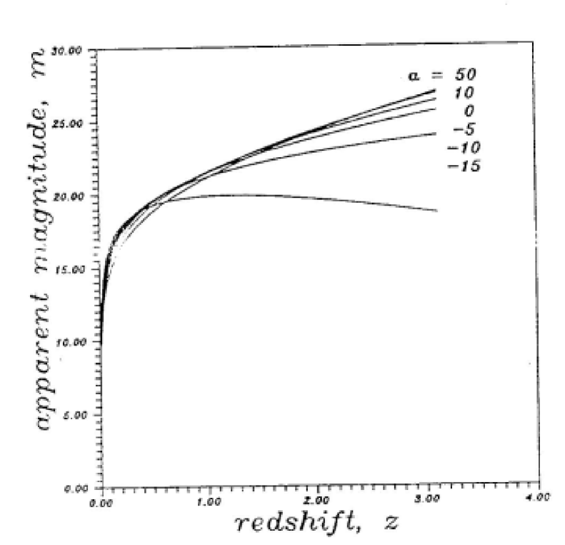
Figure 1: A plot of the redshift-magnitude relation for the model MI given by the formulas (5.6)-(5.7). We have chosen a = -15, -10, -5, 0, 10, 50 $km^{2}/s^{2}Mpc$, $b=1km/s$, d = 0 with $\tau_{0}=0.02$ $sMpc/km$ and $M=-23.5$. The effect of non-uniform pressure is similar to the effect of spatial curvature (expressed in terms of the deceleration parameter $q_{0}$) in FRW models.

The redshift-magnitude relations for the cases (5.6)-(5.7) are plotted in 1. We have chosen the age of the universe $\tau_{0}=0.02$ [sMpc/km], $M=-23.5$ and the constants $a,b,d$ are taken in the following units: [a] = $km^{2}/(s^{2}Mpc)$, [b] = km/s and [d] = Mpc. From Fig.1 one can conclude that the effect of acceleration (2.23) is similar to the effect of curvature (expressed in terms of deceleration parameter $q_{0}$) in the Friedman models. Although we plotted the relation for arbitrary $z$ we have to remember that we dropped the terms ${\bf O}\left(z^{2}\right)$, so the results can be slightly different for large redshifts.

For the model MII from (4.17) and (4.18) we have

$$u_{a;b}K^{a}K^{b}\mid_{0} = \frac{R_{,\tau}}{R}\mid_{0},$$ (5-8)

$$u_{a;bc}K^{a}K^{b}K^{c}\mid_{0} = 2\left(\frac{R_{,\tau}}{R}\right)^{2}\mid_{0}-\left(\frac{R_{,\tau}}{R}\right)_{,\tau}\mid_{0}-\frac{1}{2}c^{2}\frac{\alpha\beta}{R}\mid_{0},$$ (5-9)

and from (4.1)

$$m_{bol}=M-5\log_{10}{\tilde{H}_{0}}+5\log_{10}{cz}+1.086\left(1-\tilde{q_{0}}+\frac{9}{8}c^{2}\alpha\tau_{0}^{\frac{4}{3}}\right)z,$$ (5-10)

where

$$\tilde{H_{0}} \equiv \frac{R_{,\tau}}{R}\mid_{0}\hskip 4.2679pt=\frac{2}{3\tau_{0}},$$ (5-11)

$$\tilde{q_{0}} \equiv -\frac{RR_{,\tau\tau}}{R^{2}_{,\tau}}\mid_{0}\hskip 4.2679pt=\frac{1}{2}.$$ (5-12)

are the Friedman values of the Hubble constant and the deceleration parameter. In the Friedman limit $\alpha\rightarrow 0$ we have

$$m_{bol}=M+25-5\log_{10}{\left(\frac{2}{3\tau}\right)_{0}}+5\log_{10}{(cz)}+0.543z,$$ (5-13)

which corresponds to Eq.(41) of Da̧browski and Stelmach (1989) for the flat model $\tilde{q_{0}}=\frac{1}{2}$.

In the model MII we have only one free parameter $\alpha$ which describes inhomogeneity of the model. It can both be negative and positive and its effect on the redshift-magnitude relation is similar to the effect of curvature in FRW case (i.e. the values of $q_{0}$). In Fig.2 we plot suitable relations for different $\alpha$ given in units $(km/sMpc)^{-\frac{4}{3}}$ , $M=-23.5$ and $\tau_{0}^{-1}=75$ km/(sMpc). The main difference between the models MI and MII is that in MII the curves for different $\alpha$ become separated for redshifts approximately larger than 0.3 while in MI they differ almost from the beginning. It is the result of the fact that in the latter model the constants a, b, d effects the generalized Hubble constant (5.4) more strongly.

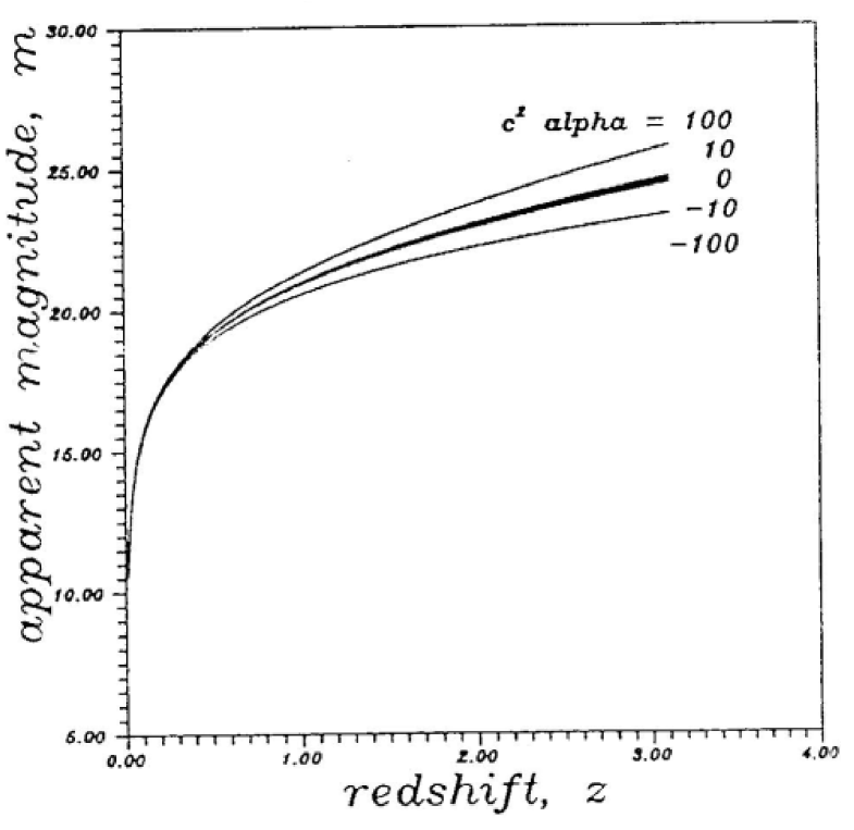
Figure 2: A plot of the redshift-magnitude relation for the model MII given by the relation (5.10). Here $\alpha c^{2}=0,\pm 10,\pm 100(km/sMpc)^{-\frac{4}{3}}$, $\tau_{0}^{-1}=75km/sMpc$ and $M=-23.5$. The effect of non-uniform pressure is similar to the effect of spatial curvature (expressed in terms of the deceleration parameter $q_{0}$) in FRW models.

b) non-centrally placed observers

For non-centrally placed observers $r_{0}\neq 0$ and $h\neq 0$ in (2.19)-(2.22) and the redshift-magnitude relation depends on the direction of a galaxy in the observer sky. According to (4.26)-(4.27) the relation (4.1) for MII reads as

$$m_{bol}=M+25-5\log_{10}{\left[\left(\frac{R_{,\tau}}{R}\right)_{0}+\frac{1}{2}c\frac{\alpha\beta}{c}r_{0}\cos{\phi}\right]}+5\log_{10}{(cz)}+4.344z+1.086z\times$$

$$\left[\frac{-2\left(\frac{R_{,\tau}}{R}\right)^{2}+\left(\frac{R_{,\tau}}{R}\right)_{,\tau}\left(1-\frac{\alpha\beta}{4}Rr_{0}^{2}\right)-\frac{11}{2}c\alpha\beta\frac{R_{,\tau}}{R}r_{0}\cos{\phi}+c^{2}\frac{\alpha\beta}{2R}\left(1-\frac{3}{4}\alpha\beta Rr_{0}^{2}\right)\cos^{2}{\phi}}{\left(\frac{R_{,\tau}}{R}+\frac{1}{2}c\alpha\beta r_{0}\cos{\phi}\right)^{2}}\right]$$

or with $R(\tau)$ given explicitly by (2.15)

$$m_{bol}=M+25+5\log_{10}{\left[\frac{cz}{\frac{2}{3}\frac{1}{\tau_{0}}+\frac{1}{2}c\alpha\beta r_{0}\cos{\phi}}\right]}+1.086z\times$$

$$\left[\frac{\frac{2}{9}\frac{1}{\tau_{0}^{2}}\left(1+\frac{3}{4}\alpha\beta^{2}\tau_{0}^{\frac{2}{3}}r_{0}^{2}\right)-c\alpha\beta\frac{r_{0}}{\tau_{0}}\cos{\phi}+\frac{1}{2}c^{2}\alpha\tau_{0}^{-\frac{2}{3}}\left(1-\frac{5}{4}\alpha\beta^{2}\tau_{0}^{\frac{2}{3}}r_{0}^{2}\right)\cos^{2}{\phi}}{\left(\frac{2}{3}\frac{1}{\tau_{0}}+\frac{1}{2}c\alpha\beta r_{0}\cos{\phi}\right)^{2}}\right].$$ (5-14)

In Figures 3-5 we plot the dependence of the redshift-magnitude relation (5.14) on the direction of the source in the sky and the distance from the center of symmetry $r_{0}$. We fix the redshift of the source to be z = 0.1, 0.5 and 1.0 correspondingly and the other parameters are the following: $\alpha c^{2}=10(km/sMpc)^{-\frac{4}{3}},\beta=1.1\cdot 10^{5}(km/s)^{\frac{2}{3}}Mpc^{\frac{1}{3}},\tau_{0}^{-1}=75km/(sMpc),-1<\cos{\phi}<1$. One can easily notice that unlikely to the case of the centrally placed observer the constant $\beta$ effects the redshift-magnitude relation as well. In fact, it is the constant which appears in the flat dust-filled Friedman limit of the Stephani Universe $\alpha\rightarrow 0$ (cf.(2.15)) and it has the same dimension. In the Friedman model its value is $\beta=1.1\cdot 10^{5}(km/s)^{\frac{2}{3}}Mpc^{\frac{1}{3}}$ for $\tau_{0}^{-1}=75km/(sMpc)$ i.e. $H_{0}=50km/(sMpc)$. From the Figures 3-5 we can see that for strongly non-centrally placed observers the redshift-magnitude relation (for fixed $r_{0}$) becomes more and more asymmetric. The smallest apparent magnitude is for the galaxies for which the angle $\phi=\pi$ ($\cos{\phi}=-1$) and they are just behind the centre of symmetry with respect to the observer. The largest apparent magnitude is achieved for $\phi=0$ ($\cos{\phi}=1$) and the galaxies are in front of the centre of symmetry with respect to the observer. For the sake of comparison (although we cannot take the limit $\alpha\rightarrow 0$ without taking $r_{0}=0$) we also draw the Friedman values of the apparent magnitude which is not dependent on the angle $\phi$.

For the non-centrally placed observer one can think about a modification of the centrally placed picture given in Fig. 2 in such a way that for each value of the redshift $z$ we draw an ”error” bar which range is given by the appropriate values of $m(z)$ given by the non-centrally placed picture of figures similar to Figures 3-5. This suggests one of the ways to explain the well-known noncompatibility of the theoretical curve with the observational data for large redshift galaxies in the Friedman universe. However, we emphasize that we do not take any evolutionary effects into account here.

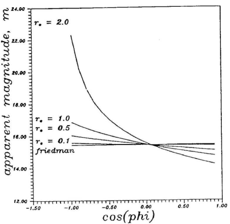
Figure 3: A plot of the dependence of the apparent magnitude on the direction in the sky for the model MII according to the formula (5.14). We fix the redshift of a galaxy to be $z=0.1$ and $\alpha c^{2}=100(km/sMpc)^{-\frac{4}{3}}$, $\beta=1.1\cdot 10^{5}(km/s)^{\frac{2}{3}}Mpc^{\frac{1}{3}}$, $\tau_{0}^{-1}=75km/(sMpc)$, $-1<\cos{\phi}<1$ and $r_{0}=0.1,0.5,1.0,2.0$. If $\cos{\phi}=-1$ galaxies are just behind the centre of symmetry with respect to the observer and the apparent magnitude is small. If $\cos{\phi}=1$ galaxies are in front of the centre of symmetry and the apparent magnitude is large. The symmetric Friedman value is given as well.

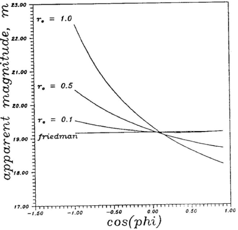
Figure 4: A plot of the dependence of the apparent magnitude on the direction in the sky for the model MII according to the formula (5.14). We fix the redshift of a galaxy to be $z=0.5$ and $\alpha c^{2}=100(km/sMpc)^{-\frac{4}{3}},\beta=1.1\cdot 10^{5}(km/s)^{\frac{2}{3}}Mpc^{\frac{1}{3}},\tau_{0}^{-1}=75km/(sMpc),-1<\cos{\phi}<1$ and $r_{0}=0.1,0.5,1.0$.

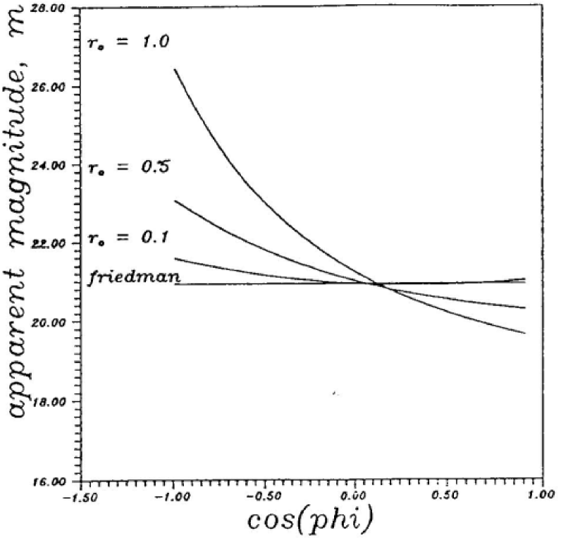
Figure 5: A plot of the dependence of the apparent magnitude on the direction in the sky for the model MII according to the formula (5.14). We fix the redshift of a galaxy to be $z=1.0$ and $\alpha c^{2}=100(km/sMpc)^{-\frac{4}{3}},\beta=1.1\cdot 10^{5}(km/s)^{\frac{2}{3}}Mpc^{\frac{1}{3}},\tau_{0}^{-1}=75km/(sMpc),-1<\cos{\phi}<1$ and $r_{0}=0.1,0.5,1.0$.

6 Discussion

The comparison of the models MI and MII with astronomical data requires a couple of conditions which have to be satisfied. For small redshift objects there should not be any problem because our models deviate in a very clear way from the flat Friedman universes but some difficulty might be related to a position of the centre of symmetry from the observer (cf. Goicoechea and Martin-Mirones 1987). Also, for some choices of the Stephani parameters the singularities of pressure may appear (cf. Da̧browski 1993). For large redshift galaxies and quasars the problem appears since the Kristian-Sachs method of Section 4 generally valids if suitable series for observational quantities are convergent. It seems to happen in the cases considered in this paper, but in general it might not be so. Of course we have still some freedom of a choice of functions $R(\tau)$ and $V(\tau,r)$ (cf. (2.2)-(2.4)) in order to make the series convergent. On the other hand for large redshift objects the evolutionary effects ought to be taken into account.

Of course the full information about the series can be obtained by calculating the second and higher order corrections to m(z) in (4.1), but the result contains the second and higher covariant derivatives of (4.2) (i.e. $u_{a;bcd}$ - see Ellis and MacCallum (1970)) and the final formula is much more complicated than the formulas (4.24)-(4.27). We decided to skip this calculations in this paper and present them, if necessary, later.

The redshift formula (3.2) is always fulfilled, but with half of the quantities taken at a galaxy position, which means that it is practically useless for observational verification.

Appendix A Tangent vector to zero geodesic for Stephani models

If $k^{a}=\frac{dx^{a}}{ds}$, where $x^{a}=(t,r,\theta,\varphi)$ and s - a parameter, is the null tangent vector to zero geodesic connecting observer (index ”O”) and galaxy (index ”G”), then the geometric optics equations for the unknown components $k^{t}$ and $k^{r}$ in the spherically symmetric Stephani universe (2.1) are

$$F^{2}\left[\left(\frac{V}{R}\right)^{\cdot}\right]^{2}\left(k^{t}\right)^{2}=\left(k^{r}\right)^{2}+h^{2}\frac{V^{4}}{R^{4}r^{2}},$$ (A1)

$$\dot{k}^{t}k^{t}+k^{t}_{,r}k^{r}+2\left(\frac{\dot{R}}{R}-\frac{\dot{V}}{V}\right)\left(k^{t}\right)^{2}+\left[\frac{\dot{F}}{F}+\frac{\left(\frac{V}{R}\right)^{\cdot\cdot}}{\left(\frac{V}{R}\right)^{\cdot}}\right]\left(k^{t}\right)^{2}$$

$$-2\left[\frac{V_{,r}}{V}-\frac{\left(\frac{V}{R}\right)^{\cdot}_{,r}}{\left(\frac{V}{R}\right)^{\cdot}}\right]k^{t}k^{r}=0,$$ (A2)

$$\dot{k}^{r}k^{t}+k^{r}_{,r}k^{r}+2\left(\frac{\dot{R}}{R}-\frac{\dot{V}}{V}\right)k^{t}k^{r}-2\left[\frac{V_{,r}}{V}-\frac{\left(\frac{V}{R}\right)^{\cdot}_{,r}}{\left(\frac{V}{R}\right)^{\cdot}}\right]\left(k^{r}\right)^{2}$$

$$-h^{2}\frac{V^{4}}{R^{4}r^{2}}\left(\frac{1}{r}-\frac{V_{,r}}{V}\right)=0,$$ (A3)

while $k^{\theta}=0$ and

$$k^{\varphi}=h\frac{V^{2}}{R^{2}r^{2}},$$ (A4)

The easiest solutions of (A.1)-(A.4) are (Da̧browski 1993):
a) if $\left(\frac{V}{R}\right)^{\cdot\cdot}=0$ i.e. $k(t)=\left(ct+d\right)R(t)$ and $R(t)=\left(at+b\right)^{-1}$ ,$a,b,c,d=const.$, then

$$k^{t} = \frac{V^{2}}{FR^{2}}\frac{1}{\left[\left(\frac{V}{R}\right)^{\cdot}\right]^{2}},$$ (A5)

$$k^{r} = \pm\frac{V^{2}}{R^{2}}\sqrt{\frac{1}{\left[\left(\frac{V}{R}\right)^{\cdot}\right]^{2}}-\frac{h^{2}}{r^{2}}}.$$ (A6)

b) if $\left(\frac{V}{R}\right)^{\cdot}_{,r}=0$ i.e. $\left(\frac{k}{R}\right)^{\cdot}=0$, then

$$k^{t} = \frac{V^{2}}{FR^{2}}\frac{1}{\left(\frac{V}{R}\right)^{\cdot}},$$ (A7)

$$k^{r} = \pm\frac{V^{2}}{R^{2}}\sqrt{1-\frac{h^{2}}{r^{2}}}.$$ (A8)

If we use the Friedman-like time coordinate (2.9) we have to change the derivative with respect to t into the derivative with respect to $\tau$ in (A.1)-(A.8).

Appendix B A redshift-magnitude relation for a radial ray

From (A.1) one can easily conclude that for moving radially towards or away from the centre ray $\left(h=0\right)$ the ratio of components $k^{t}$ and $k^{r}$ of the tangent vector is given by

$$\frac{k^{r}}{k^{t}}=\pm D\frac{V}{R}=\pm\left(\frac{V}{R}\right)^{\cdot},$$ (B1)

and $k^{\theta}=k^{\varphi}=0$. This might be useful for calculating the redshift-magnitude relation. From (4.11)-(4.12) together with (B.1) we have

$$u_{a;b}K^{a}K^{b}=-\frac{1}{F}\pm\frac{D_{,r}}{D}\frac{V}{R},$$ (B2)

and

$$u_{a;bc}K^{a}K^{b}K^{c}=\frac{1}{D}\left(\frac{1}{F}\right)^{\cdot}+\frac{2}{F^{2}}\mp\frac{4}{F}\left(\frac{D_{,r}}{D}\right)\frac{V}{R}+\left(\frac{D_{,r}}{D}\right)^{2}\frac{V^{2}}{R^{2}}$$

$$\mp\left(\frac{D_{,r}}{D}\right)_{,t}\frac{V}{DR}-\left(\frac{D_{,r}}{D}\right)_{,r}\frac{V^{2}}{R^{2}}-\frac{D_{,r}}{D}\frac{V_{,r}V}{R^{2}},$$ (B3)

where

$$\frac{D_{,r}}{D}=\frac{\left(\frac{V}{R}\right)^{\cdot}_{,r}}{\left(\frac{V}{R}\right)^{\cdot}}-\frac{\left(\frac{V}{R}\right)^{\cdot}}{\left(\frac{V}{R}\right)},$$ (B4)

and the first signs refer to outgoing rays and the second to incoming rays ( $\frac{k^{r}}{k^{t}}=\frac{\frac{dr}{ds}}{\frac{dt}{ds}}=\frac{dr}{dt}$ so ”+” for outgoing and ”-” for incoming rays respectively).

References

- (1) Bondi,H.1947, Monthly Not. R. Astr. Soc.,107,410
- (2) Bonnor,W.B.,1974, Monthly Not. R. Astr. Soc.,167,55
- (3) Da̧browski,M.P.,1993, Journ.Math.Phys.,34,1447
- (4) Da̧browski,M.P. & Stelmach J.,1989, Astron. J.,97, 978 (astro-ph/0410334)
- (5) Dyer,C.C.,1979, Monthly Not. R. Astr. Soc. 189,189
- (6) Ehlers,J.,1961,Akad.Wiss.Lit.(Mainz),11,792 (for English translation see: 1993, Gen.Rel.Grav.,25,1225)
- (7) Ellis,G.F.R. & MacCallum,M.A.H.,1970,Commun.Math.Phys.,19,31
- (8) Goicoechea,L.J. & Martin-Mirones,J.M.,1987,A&A,186,22
- (9) Hellaby C. & Lake K.,1984,ApJ,282,1
- (10) Hellaby C. & Lake K.,1985,ApJ,290,381
- (11) Hellaby C.,1987,Class.Quantum Grav.,4,635
- (12) Hellaby C.,1988,Gen.Rel.Grav.,20,1203
- (13) Kramer D., Stephani H., MacCallum M. A. H., Hertl E.,1980, Exact Solutions of the Einstein Field Equations (CUP, Cambridge)
- (14) Krasiński,A.,1983,Gen.Rel.Grav.,15,673
- (15) Krasiński,A.,1997, Inhomogeneous Cosmological Models (CUP, Cambridge)
- (16) Kristian,J. & Sachs,R.K.,1966,ApJ,143,379
- (17) Linde,A.A.,1994,Phys.Rev.,D50,2456
- (18) Moffat,J.W., & Tatarski,D.C.,1992,Phys.Rev.,D45,3512
- (19) Partovi,M.H. & Mashhoon,B.,1984,ApJ,276,4
- (20) Roeder,R.C.,1975,ApJ,196,671
- (21) Quevedo,H. & Sussman,R.A.,1995,Journ.Math.Phys. 36, 1353 (gr-qc/9411021)
- (22) Quevedo,H. & Sussman,R.A.,1995,Class.Quantum.Grav. 12,859 (gr-qc/9411022)
- (23) Sussman,R.A.,1994,Class. Quantum Grav.,11,1445
- (24) Tolman,R.C.,1934,Proc.Natl.Acad.Sci.,20,169
- (25) Vilenkin,A.,1985,Phys.Rep.,121,265
- (26) Weinberg,S.,1989,Rev.Mod.Phys.,61,1
- (27) Wesson,P.S. & Ponce de Leon,J.,1989,Phys.Rev.,D39,420