Photoassociative molecular spectroscopy for atomic radiative lifetimes.

Abstract

When the atoms of a dimer remain most of the time very far apart, in so-called long-range molecular states, their mutual interaction is ruled by plain atomic properties. The high-resolution spectroscopic study of some molecular excited states populated by photoassociation of cold atoms (photoassociative spectroscopy) gives a good illustration of this property. It provides accurate determinations of atomic radiative lifetimes, which are known to be sensitive tests for atomic calculations. A number of such analyses has been performed up to now, for all stable alkali atoms and for some other atomic species (Ca, Sr, Yb). A systematic review of these determinations is attempted here, with special attention paid to accuracy issues.

1 Introduction

The precise knowledge of atomic radiative lifetimes is a prerequisite for many problems of modern quantum physics. First of all, their measurement often represents an accurate check for ab initio calculations of atomic structure [1, 2, 3]: indeed, their computed values are much more sensitive to the details of the electronic wave functions than the computed total energy. The reliability of such calculations is essential when atoms are used for the investigation of fundamental problems, like the search for parity non-conservation effects which are predicted by theories beyond the Standard Model. Up to now, the strongest constraint on the magnitude of such effects is provided by experiments with cesium [4, 5, 6] for parity violation, or with thallium atoms [7] for time-reversal symmetry violation which would manifest itself by a permanent electric dipole moment of the electron.

Among all atomic species, the alkali atoms are systems of choice for comparative experimental and theoretical studies: their main resonant transition ${}^{2}S\rightarrow$${}^{2}P$ lies in the optical domain, while calculations are facilitated by their simple electronic structure. At the 5^th ASOS conference in Meudon (France) in 1995, U. Volz and H. Schmoranzer presented a review on measurements and calculations of alkali atom radiative lifetimes, as well as a series of updated precision measurements of the radiative lifetimes for Li, Na, K, and Rb atoms using beam-gas-laser spectroscopy [8]. In particular, they solved a long-standing discrepancy between ab-initio calculations and measurements for lithium and sodium. In their paper, they refered to the first measurement of a radiative lifetime using the emerging technique of photoassociative spectroscopy (PAS) on ultracold lithium atoms [9]. Their result was in good agreement with the PAS one, while the error bar derived with the PAS technique was claimed to be four times smaller than their own.

More than a decade later, and motivated by our recent work on the radiative lifetime of atomic cesium [10], we take the opportunity offered by the edition of the special issue of Physica Scripta for the 9^th ASOS conference, to review the status and the accuracy of the PAS approach for determining the radiative lifetimes of alkali atoms, and more generally of atomic species which are nowadays laser-cooled and trapped. In Section 2, we briefly describe the photoassociation process which allows the investigation of the long-range interaction within a pair of cold atoms, focussing on its link with the energy-level spacing of the atom pair through the so-called LeRoy-Bernstein law, and with the atomic radiative lifetime. Next (Section 3) we focus on a specific class of electronic states of the atom pair - the so-called ”pure long-range” states - which are particularly relevant for the extraction of Na [11], K [12], Rb [13, 14] and Cs [15, 10] radiative lifetimes from PAS of these unusual molecular states. The case of molecular states which are not of the pure long-range class is described in Section 4. Two different methods have been used to derive accurate radiative atomic lifetimes from PAS performed in cold samples: a direct application of the LeRoy-Bernstein asymptotic law has been used in the cases of Sr [16] and Yb [17]; a global fit of the full molecular potential at both short and large distances has been performed to extract the radiative lifetimes for Li [18], Ca [19] and Sr [20] atoms. The last section is devoted to the sensitive issue of the evaluation of the accuracy of the results for the various species obtained by PAS, which is generally claimed to be better than the one obtained from standard atomic physics techniques.

2 Photoassociation of cold atoms, photoassociation spectroscopy and long-range interactions

2.1 Basics of photoassociation process

Photoassociation (PA) in atomic vapors is a well-known process [21, 22, 23, 24]: a pair of atoms (M,M’) absorbs a photon of suitable energy $h\nu_{PA}$, generally red-detuned from the energy of an atomic transition $h\nu_{0}$, to create molecules in rovibrational levels of an excited electronic state according to the reaction: $M+M^{\prime}+h\nu_{PA}\rightarrow(MM^{\prime})^{*}$. At room temperature, the PA process is not selective in the final state, due to the width of the Maxwell-Boltzmann kinetic energy distribution of the atoms, which is most often larger than the energy gap between consecutive molecular levels. Shortly after the first experimental observations of laser-cooling of atoms, Thorsheim et al [25] proposed to perform photoassociation of ultracold atoms: as the width of the kinetic energy distribution of the cold atoms is comparable or even smaller than the natural width of the excited state, the free-bound PA process allows a selective excitation of the initial atom pair into an excited molecular state, just like a bound-bound process would do. Then it is possible to reach rovibrational levels with large spatial extension and with small binding energy (Figure 1). PA has been observed a few years later on cold sodium [26] and rubidium [27] samples, and became soon a fantastic tool for high-resolution molecular spectroscopy, referred to as photoassociation spectroscopy (PAS) [28]. The recent review by Jones et al [29] yields a comprehensive study of PAS, and addresses one of the main issues of PA which is particularly relevant for the present paper: ”PA favors the study of physicists’ molecules, i.e., molecules whose properties can be related (with high precision) to the properties of the constituent atoms.”.

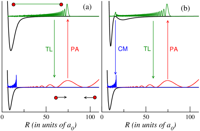
Figure 1: General scheme of the photoassociation of a pair of cold atoms in their $S$ ground state. In panel (a), the atoms interact through a molecular potential curve, with a van der Waals character at large $R$, i.e., varying as $R^{-6}$. As their relative initial kinetic energy is very small, the radial wave function has a large amplitude at large distances, so that in a classical vision, the atom pair likely absorbs a photon with a frequency red-detuned from the atomic $S\rightarrow P$ transition frequency (arrow labelled PA). Bound levels with a small binding energy and a large spatial extension are efficiently populated. Most of the relative vibrational motion then takes place at large $R$, where the excited interaction potential behaves as $R^{-3}$. This bound level can either decay back to a pair of free atoms which escape from the cold atom trap (arrow TL, for trap loss), or to a bound level of the molecular ground state, creating then a cold molecule (arrow CM, for cold molecule). Panel (b) illustrates the same process for an excited double-well potential like, for instance, in cesium photoassociation.

2.2 Long-range resonant dipole behavior

All the experiments reviewed here follow the general scheme of Figure 1. A pair of identical atoms in their ground state (either $ns$ ²S_1/2 or $ns^{2}$ ¹S₀ for alkali or alkaline-earth-like elements, respectively) is excited into a molecular state connected to the lowest ($ns$ ²S_1/2+$np$ ²P_1/2,3/2) or ($ns^{2}$ ¹S₀+$nsnp$ ¹P${}^{0}_{1}$) dissociation limit. In all these cases, the asymptotic interaction between the atoms is dominated by the resonant dipole interaction and is approximated by

$$V(R)=D-\frac{C_{3}}{R^{3}},$$ (1)

where $D$ is the dissociation energy of the interaction potential. The coefficient $C_{3}$ depends on the relative orientation of the atomic dipoles with respect to the molecular axis and is thus different for a $\Sigma$ or a $\Pi$ molecular state. It corresponds to the exchange of excitation between the two atoms and it is simply related to a characteristic of the atom, the atomic dipole matrix element. One has

$$C_{3}^{\Sigma}=-2C_{3}^{\Pi}=-2\frac{\mathcal{R}^{2}}{3},$$ (2)

where $\mathcal{R}=<ns|r|np>$ is the radial integral of the dipole length operator between the atomic $ns$ and $np$ orbitals. The $C_{3}$ coefficients are therefore related to the atomic radiative lifetime of the $P$ level since

$$\tau=\frac{9\hbar\lambda^{3}}{32\pi^{3}\mathcal{R}^{2}},$$ (3)

where $\lambda$ is the wavelength of the considered $S\rightarrow P$ atomic transition.

Equation (1) is always an approximation, only valid for very large interatomic distances. Several other effects are likely to contribute to the interaction energy:

• the following terms $C_{n}/R^{n}$ with n=6, 8, 10, …. of the multipole expansion: they account for polarization and dispersion forces;

• the spin-orbit interaction: it has to be taken into account for alkali atoms, but not for alkaline-earth and alkaline-earth-like ones, due to the choice of the excited state;

• the hyperfine structure of the ground state: for alkali atoms, the hyperfine splitting of the excited atomic state increases with atomic mass; it is almost negligible at the experimental precision of PAS for lithium but not for cesium; the lack of the hyperfine structure for the chosen isotopes of the other elements considered here, Ca, Sr and Yb, simplifies the analysis of the experiments;

• the rotation of the molecule: it is often absent in the initial colliding state, when the temperature of the atom cloud is low enough ($s$-wave collisions); however it has always to be accounted for in the excited molecular state. The rotational energy $E^{rot}(v,J)$ of a rovibrational level $(v,J)$ can be estimated by the diagonal part of the rotational Hamiltonian

  $$H^{rot}=\frac{\mathbf{J}^{2}-2\mathbf{J}.\mathbf{j}+\mathbf{j}^{2}}{2\mu R^{2}},$$ (4)

  where $\mathbf{J}$ and $\mathbf{j}$ are, respectively, the total angular momentum and the total electronic angular momentum of the considered dimer and $\mu$ its reduced mass;

• the overlap between the two electron clouds: it is manifested by an exchange energy which vanishes exponentially with increasing atomic distances [30, 31]. For the excited states of the alkali dimers that we consider here, it depends essentially on a single parameter which is the product of the amplitudes of the atomic $ns$ and $np$ wavefunctions. The derivation of the relevant expressions of the $\Sigma$ and $\Pi$ asymptotic exchange terms, $V_{exch}^{\Sigma,\Pi}$, is recalled in Ref [15];

• the retardation effect, related to the Casimir-Polder effect in London-van der Waals interaction [32]: when accounting for the finite velocity of light, the long-range interaction between the atoms is modified. This effect is usually small but clearly noticeable in several experiments reviewed here. Following Refs [33, 34], it can be accounted for simply, by multiplying the $C_{3}$ coefficient by a correcting term which is different for $\Pi$ and $\Sigma$ states:

  $$f^{\Pi}(R) = \cos\big{(}\frac{2\pi R}{\lambda}\big{)}+\big{(}\frac{2\pi R}{\lambda}\big{)}\sin\big{(}\frac{2\pi R}{\lambda}\big{)}-\big{(}\frac{2\pi R}{\lambda}\big{)}^{2}\cos\big{(}\frac{2\pi R}{\lambda}\big{)}$$ (5)

  $$f^{\Sigma}(R) = \cos\big{(}\frac{2\pi R}{\lambda}\big{)}+\big{(}\frac{2\pi R}{\lambda}\big{)}\sin\big{(}\frac{2\pi R}{\lambda}\big{)};$$ (6)

• the intra-atomic relativistic effects: they tend to contract differently the atomic $p_{1/2}$ and $p_{3/2}$ orbitals [35]. It is possible to account for these effects through a small parameter $\epsilon$, which characterizes the ratio between the dipole matrix elements corresponding to the two $p$ orbitals

  $$\frac{<ns|r|np_{3/2}>^{2}}{<ns|r|np_{1/2}>^{2}}=\frac{2\tau_{1/2}}{\tau_{3/2}}\Big{(}\frac{\lambda_{3/2}}{\lambda_{1/2}}\Big{)}^{3}=\frac{2}{(1+\epsilon)^{2}}.$$ (7)

  More details can be found in rubidium [14] and cesium [15, 10] studies;

• the non-adiabatic terms negelected in the Born-Oppenheimer approximation, which assumes fixed nuclei of infinite mass: it is possible [36] to release this assumption while still maintaining the decoupling of nuclear and electronic motions, by considering the diagonal corrections for the motion of the nuclei. The description of these terms can be found in Ref [18];

• the specific shift and broadening of the PA lines due to the temperature of the atomic cloud: these effects depend also on the shapes of the ground and excited molecular potentials. They are discussed in great detail in the calcium study [19];

• the so-called predissociation process: it is due to the interaction of the molecular state with the continuum of a neighboring one and it gives rise to line broadening. This problem arose in particular in the ytterbium study [17].

2.3 LeRoy-Bernstein law and energy spacing of high-lying vibrational states

Assuming that the asymptotic form of the molecular potential is written as

$$V(R)=D-\frac{C_{n}}{R^{n}},$$ (8)

one can show, using a semi-classical Wigner-Kramers-Brillouin (WKB) description of the vibrational wavefunction, that the energy $E_{v}$ of a molecular vibrational level is related to its vibrational quantum number $v$ through the so-called LeRoy-Bernstein law [37]:

$$(D-E_{v})=[X_{n}(v_{D}-v)]^{(2n/n-2)}$$ (9)

(10)

$$X_{n}=\hbar\sqrt{\frac{\pi}{2\mu}}~{}\frac{(n-2)\Gamma(1+1/n)}{\Gamma(1/2+1/n)}~{}C_{n}^{-1/n}.$$ (11)

In Equation (11), $\Gamma(z)$ is an Euler Gamma function and $v_{D}$ is a non-integer number (the non-integer value that $v$ would take at the dissociation limit $D$) which is related to the phase accumulated by the wavefunction over its whole spatial extension, including the short-range part of the potential. In the case of a $R^{-3}$ potential, Equation (11) becomes

$$(D-E_{v})=X_{0}(v_{D}-v)^{6},$$ (12)

with

$$X_{0}=(X_{3})^{6}=\Big{[}\frac{\hbar^{2}}{2\mu}\Big{]}^{3}\Big{[}\frac{\Gamma(4/3)}{\Gamma(5/6)}\Big{]}^{6}\frac{\ pi^{3}}{(C_{3})^{2}}.$$ (13)

As the total number of vibrational levels of the potential is most often not known, it is convenient, instead of labeling the levels by a number $v$ starting from the $v=0$ lowest vibrational level, to characterize them by $v^{*}$ starting from the $v^{*}=1$ uppermost one. One has then

$$(D-E_{v})=X_{0}(v^{*}-v^{*}_{D})^{6},$$ (14)

with $v_{D}$ reduced to its fractional part $0\leq v^{*}_{D}<1$. Assuming that the density of levels allows one to introduce a continuous derivative with respect to $v$, the energy spacing between consecutive vibrational levels can be written as

$$\frac{dE}{dv}=-\frac{2n}{n-2}(X_{n})^{2n/(n-2)}(v_{D}-v)^{(n+2)/(n-2)}$$ (15)

or, in the $n=3$ case,

$$\frac{dE}{dv^{*}}=-6X_{0}(v^{*}-v^{*}_{D})^{5}$$ (16)

and appears thus as depending directly on $X_{0}$, i.e. on $C_{3}$ (Equation (13)): one clearly sees how the analysis of PAS data allows one to extract the atomic lifetime from the energy spacing of high-lying levels.

2.4 Pure long-range states: molecules as atom pairs

For Na₂, K₂, Rb₂ and Cs₂ dimers, the molecular state of $0_{g}^{-}$ symmetry converging toward the first ($ns+np_{3/2}$) limit is a ”pure long-range” state according to the definition of Ref [38]. It has a double-well potential, for which the most external well is shallow and entirely located at unusually large internuclear separations. Each atom keeps somehow its identity and the molecule looks more like a pair of atoms. The electron cloud overlap is unimportant, so that the potential is completely determined by long-range interatomic forces and atomic spin-orbit splitting, and can thus be calculated with high precision. We emphasize here that this situation is very different from the one encountered with usual molecular potentials, for which the knowledge of the inner part of the potential curve most often relies on quantum chemistry calculations, which never reach such a precision.

The dominant long-range interactions are the $R^{-3}$ resonant dipole interaction and the spin-orbit coupling [39]. For the $0_{g}^{-}$ potentials, the simple analytical model introduced in [40] is the basis of the analysis. Two $0_{g}^{-}$ potentials arise from a mixing of two Hund’s case (a) states, a repulsive ${}^{3}\Pi_{g}$ state and an attractive ${}^{3}\Sigma_{g}^{+}$ one. The two adiabatic $0_{g}^{-}$ potentials are obtained by diagonalizing the matrix of the interaction in this basis of states,

$$\hskip 49.79231pt\Pi\hskip 49.79231pt\Sigma$$

$$V_{MP}(R) = \left(\begin{array}[]{cc}V^{\Pi}(R)-\frac{2\Delta}{3}&\frac{\sqrt{2}\Delta}{3}\\ \frac{\sqrt{2}\Delta}{3}&V^{\Sigma}(R)-\frac{\Delta}{3}\end{array}\right)\begin{array}[]{ll}\Pi\\ \Sigma\end{array},$$ (21)

with

$$V^{\Pi/\Sigma}(R)=-\frac{C_{3}^{\Pi/\Sigma}}{R^{3}}f^{\Pi/\Sigma}(R)-\frac{C_{6}^{\Pi/\Sigma}}{R^{6}}-\frac{C_{8}^{\ Pi/\Sigma}}{R^{8}}+V_{exch}^{\Pi/\Sigma},$$ (22)

where $\Delta$ is the atomic spin-orbit splitting and the zero of energy is taken at the ($ns+np_{3/2}$) asymptote. The $0_{g}^{-}$ potential in which we are interested is the upper adiabatic potential, which converges to the ($ns+np_{3/2}$) limit. As this state is a mixture with $R$-varying weights of two states having different coefficients of the $R^{-3}$ term, it is clear that one has an ”effective” $C_{3}$ which varies with $R$ and that the validity of the LeRoy-Bernstein law is limited by the mixing of states. The knowledge of the eigenvectors of the matrix of Eq.(21) allows one to evaluate the corrections which involve the $R$-dependent mixing of states, like the $\mathbf{j}^{2}$ term of Equation (4), or which contain $R$-derivatives, like the non Born-Oppenheimer corrections. The determination of the parameters entering in the matrix of Eq.(21), where it is possible to add all the effects previously described (see for instance [14]), yields an analytical expression for the $0_{g}^{-}$ potential.

3 Determination of the radiative lifetime of Na, K, Rb, Cs atoms from pure long-range state analysis

Table 1 summarizes the values of the atomic radiative lifetimes of the first excited $np$ states of Na, K, Rb and Cs which have been obtained through photoassociation of laser cooled atoms in the pure long-range $0_{g}^{-}$ state of the corresponding dimer, together with other recent high-precision measurements using various methods.

Table 2 displays the main characteristics of these different studies. Since the $0_{g}^{-}$ potential is a pure long-range potential, one does not need to find a way to deal with an inner part of the potential in order to avoid reducing the precision, as it would be the case for a ”normal” potential. In all studies, the retardation effect has been introduced according to Equation (6). For light atoms retardation has been found impossible to ignore: PAS of the $0_{g}^{-}$ state of Na₂ provided the first reported evidence of such effects in molecular spectra and an estimation of the retardation contribution for different alkali dimers [11]. In the case of heavier atoms, the effect is less important. For cesium, a fit without retardation yields parameters which are not significantly different from the ones of Ref [10], which included retardation. Besides resonant dipole and spin-orbit interaction, which are always the dominant terms, the terms of the multipole development in $R^{-6}$ and $R^{-8}$ are introduced in all studies, but the corresponding parameters, or ratios between them are sometimes kept fixed to a theoretical value (see Table 2). The $R^{-10}$ term is generally negelected, except in Ref [13], where its influence is discussed. The influence of molecular rotation is accounted for in all studies, in the form given by Equation (4). Slightly different ways of dealing with the mixing of $\Pi$ and $\Sigma$ states have been used, as we will see below. Asymptotic exchange interaction has to be introduced for the heavier elements, Rb and Cs. The variation with $R$ of the spin-orbit interaction was considered in Refs [14, 15]. Finally the validity of the Born-Oppenheimer approximation is carefully investigated in the sodium study [11]. Hyperfine structure does not appear in PA spectra, except for very high-lying levels. As it is neither resolved in the experiments nor introduced in the models used for the lifetime value extraction, it constitutes an important limitation to the final precision of the determinations.

Table 1: Determinations from photoassociation spectroscopy (PA) of the radiative lifetimes of the atomic $np^{2}P_{3/2}$ states of Na, K, Rb and Cs (in bold face), together with recent measurements by other methods. We quote only references dating from 1994 or later; a good review on precision lifetime measurements on alkali atoms up to 1996 can be found in [8]. For the experiments involving PA of cold atoms, the atom cloud temperature is recalled, in parenthesis. For rubidium, the value noted ^∗, attributed to Ref [41], is calculated using their result for $<s|r|p_{1/2}>*<s|r|p_{3/2}>$ together with the ratio of the $5p^{2}P_{1/2}$ and $5p^{2}P_{3/2}$ lifetimes of Ref [8]. For cesium, the value, noted ^∗∗, from Ref [42], is based on an experimental determination of the $C_{6}$ van der Waals coefficient of the ground molecular state [43] and on a theoretical relationship between this coefficient and the $C_{3}$ coefficients.

element	author(date)	ref	$\tau_{3/2}$ (ns)	method
Na($3s-3p$)	Jones et al. (1996)	[11]	16.230(16)	PA ($500~{}\mu$K)
	Oates et al. (1996)	[44]	16.237(35)	linewidth
	Tiemann et al. (1996)	[45]	16.222(53)	mol spectr
	Volz et al. (1996)	[8]	16.254(22)	fast beam
K($4s-4p$)	Wang et al. (1997)	[12]	26.34(5)	PA ($500~{}\mu$K)
	Volz et al. (1996)	[8]	26.45(7)	fast beam
Rb($5s-5p$)	Freeland et al. (2001)	[13]	26.24(7)	PA ($700~{}\mu$K)
	Gutteres et al. (2002)	[14]	26.33(8)	PA ($120~{}\mu$K)
	Volz et al. (1996)	[8]	26.24(4)	fast beam
	Boesten et al. (1997)	[41]	26.67(34)∗	PA ($\sim$mK)
	Simsarian et al. (1998)	[46]	26.20(9)	photon counting
Cs($6s-6p$)	Amiot et al. (2002)	[15]	30.462(3)	PA ($300~{}\mu$K)
	Bouloufa et al. (2007)	[10]	30.41(30)	PA ($300~{}\mu$K)
	Young et al. (1994)	[47]	30.41(10)	pulsed laser
	Rafac et al. (1999)	[48]	30.57(7)	fast beam
	Derevianko et al. (2002)	[42]	30.39(6)∗∗	from C6

Table 2: Comparison of the determinations of atomic lifetimes from photoassociative spectroscopy of the $0_{g}^{-}$ states. The most important points are recalled, when available. Displayed here are: the estimated experimental uncertainty on the measured energy of the vibrational states (in MHz), $\sigma_{E}$; the number of levels included in the fitting procedure, $N$; the smallest and largest values of the external Condon points of these levels, $R_{Cmin}$ and $R_{Cmax}$ (1$a_{0}=$0.0529277 nm); the energy terms that were included in the asymptotic potential in the considered analysis: non-Born-Oppenheimer (non-BO), exchange (exch.) or relativistic (rel.) terms; the ”effective” number of free parameters included in the fit, $p$ (i.e. the number of parameters of the model decreased by one each time either a parameter or a ratio between two parameters is kept fixed); the $\chi^{2}$ value of the fit (eventually recalculated to fit the definition of Equation (24)), when it is available; the estimated relative uncertainty of the $np_{3/2}$ radiative lifetime, $\sigma_{\tau}$ (in $\%$), as given in the original reference. The values of $R_{Cmin}$ correspond to the bottom of the external well. The value of $R_{Cmax}$ noted ^∗ for Na has been calculated from the value of the binding energy of the highest level included in the fit (similar data were not available for potassium); for Rb (resp. Cs), the values of $R_{Cmax}$ are deduced from the corresponding $v$ value using [49] (resp. [50]).

atom	$\sigma_{E}$ (MHz)	$N$	$R_{Cmin}$(a0)	$R_{Cmax}$(a0)	energy terms	$p$	$\chi^{2}$	$\sigma_{\tau}$($\%$)
23Na [11]	5	7	70	122∗	non-BO	2		0.1
39K [12]	$<$60	23	52		non-BO	2	0.42	0.2
85,87Rb [13]	60	75	32	90	exch.	5	2.5	0.27
87Rb [14]	300	56	32	166	exch., rel.	8	1.1	0.3
133Cs [15]	150	75	23	65	exch., rel.	9	1.7	0.01
133Cs [10]	150	71	23	66	exch., rel.	6	0.41	1.

In all studies, calculated vibrational energies are finally fitted to $N$ chosen experimental data with $p$ free parameters. Uncertainty is given for the lifetime value, which sometimes includes an estimation of systematic errors. Table 2 displays, when available, the experimental uncertainty $\sigma_{E}$, $N$, $p$ and the relative uncertainty on the lifetime value, $\sigma_{\tau}$. To characterize the $R$-range involved in the analysis, we present also, when it was possible to find them or to calculate them, the values of the external Condon points $R_{Cmin}$ and $R_{Cmax}$ of the lowest and highest levels included in the fit, respectively.

3.1 Sodium

The $0_{g}^{-}$ external well of Na₂ is very shallow, with only 12 vibrational levels. The energies of two rotational levels ($J=2$ and $J=4$) for $v$ values ranging from 0 to 7 were measured with an uncertainty of 5 MHz. The analysis of the data was made by starting from the model of Movre and Pichler [40] and by adding successively the most important corrections: retardation, $R^{-6}$ and $R^{-8}$ terms, non-adiabatic diagonal corrections and rotation. In addition to the $B_{v}J(J+1)$ term, corresponding to the $\mathbf{J}^{2}$ term of Equation (4), the authors calculated the $\mathbf{j}^{2}$ term by using the previously calculated mixing of $\Sigma$ and $\Pi$ states.

This progressive introduction of the energy terms allowed the authors to clearly point out the role of the different corrections, in particular of the retardation effect: they were able to give an accurate estimation of the contribution of this effect to the well depth. They also performed a complete coupled-channel calculation including all molecular potentials correlated to the ($3s+3p$) limit, which accounts for non Born-Oppenheimer effects. The long-range potentials were smoothly connected at $R=35$ a₀ to ab initio calculations. This complete calculation shows that the non Born-Oppenheimer effects are very small. The influence of the inner part of the potentials was found fully negligible (using a hard wall at 35 a₀ gave almost no shift of the relevant eigenenergies). A fit of the $J=2$ results was made while keeping constant the two $C_{8}$ coefficients (using the values of Ref [51]) and the ratio between the two $C_{6}$ ones (using the same reference). ¿From the result of this fit, a value of the $3p$ atomic radiative lifetime was deduced, which is in good agreement with the result of fast beam measurements of Ref [8] and with two other recent experimental values, based on linewidth analysis and on molecular spectroscopy of low-lying vibrational levels (see Table 1). It also agrees well with the theoretical result of Ref [1]. All these data have completely removed a long-standing discrepancy between experiment and theory (see [8]).

3.2 Potassium

A PAS study with ultracold potassium atoms was performed in 1997 [12], with a ”dark spot” magneto-optical trap. The vibrational levels of the pure long-range $0_{g}^{-}$ potential converging to the ($4s+4p_{3/2}$) limit have been observed between $v=0$ and $v=30$. The rotational component $J=2$ of most levels was measured with an uncertainty smaller than 60 MHz. The analysis is performed along the same lines as for sodium. The calculated rovibrational energies are fitted to 23 measured ones ($v=0-12,14-17,19-22,24,26$); the ratios between $C_{6}$ and $C_{8}$ coefficients are kept fixed to a theoretical value [51]. The one-$\sigma$ standard deviation is 0.0013 cm^-1. The uncertainty on the $C_{3}$ value includes both a part coming from the fitting procedure and a systematic part coming from the limitations of the model, essentially from neglecting the molecular hyperfine structure. The estimation of the final uncertainty is however not described in detail. The lifetime value agrees well with the measurement of Ref [8] (see Table 1).

3.3 Rubidium

There are two independant studies [13, 14], using different experimental data.

The first experiment [13] used a FORT trap with a temperature of about 700 $\mu$K and doubly spin-polarized atoms. From photassociation spectra of both ⁸⁵Rb and ⁸⁷Rb atoms, a large number of rovibrational energy levels of the $0_{g}^{-}$ potential of both isotopes ($v=0-40$ for ⁸⁵Rb and $v=0-24,28-35,41-47$ for ⁸⁷Rb) were obtained with an uncertainty of the order of 60 MHz. The diagonalization of the matrix of Equation (21) was done analytically on a simplified form of the matrix, before the addition of the correcting terms, some of them (non-adiabatic terms, rotation) depending on the mixing of states which is characterized by the eigenvectors of the diagonalization. The terms introduced are: retardation effect on the resonant dipole interaction, dispersion terms up to $R^{-8}$, asymptotic exchange interaction, rotation (using the known mixing of $j=0$ and $j=2$ states). Finally, the effect of $R^{-10}$ terms and of non-adiabatic corrections have been tested. A rather detailed study of these effects and of their influence on the results of the fit procedure is given: we will comment on this point in the last section.

The other study [14] has been performed on the experimental data of Ref [52], concerning only ⁸⁷Rb, in a MOT trap at about 120 $\mu$K. The analysis of the data is conducted in a similar way. The $v$ values included in the fit were $v=0,1,12-23,30-71$. The diagonalization is done numerically on the complete form of the two-state matrix given by Equation (21), including retardation effect on the resonant dipole interaction, dispersion terms up to $R^{-8}$, asymptotic exchange interaction, rotation, intra-atomic relativistic corrections and $R$-varying spin-orbit terms. Concerning rotation, the $\mathbf{j}^{2}$ term was simply calculated using the asymptotic value $j=2$. The spin-orbit $R$-variation, which was suggested by quantum chemistry calculations, appeared to greatly diminish the agreement between experimental and calculated values. The estimation of the uncertainty on the lifetime value will also be discussed in the last section.

The lifetime values obtained from the two PAS studies are fully compatible, and in agreement with most of the previous experimental determinations (see Table 1).

3.4 Cesium

In the cesium case, the two published studies [15, 10] from our group concern the analysis of the same PAS data from ref.[50], from which a Rydberg-Klein-Rees (RKR) potential was previously extracted. Our second analysis [10] was necessary in order to solve remaining discrepancies in the intensity of the PA spectrum and in the scattering length and the van der Waals ground state $C_{6}$ values that we deduced in Ref [53].

The $0_{g}^{-}$ potential of Cs₂ is not strictly speaking a pure long-range one: the minimum of the external well is located around 25 a₀, whereas the LeRoy criterion which is generally used for the definition of long-range distances [54] yields a distance of about 28.5 a₀. It was therefore unavoidable to introduce the asymptotic exchange term. The top of the potential barrier separating the internal and external well is critically related to the exchange term and is expected to be close to the energy of the dissociation limit [55]. The imperfect knowledge of the height of the barrier will affect the description of the highest levels, which were therefore not introduced in the fit. Relativistic atomic corrections were introduced and, in the first paper, $R$-variation of the spin-orbit was also considered, like in Ref [14]. Both studies used exactly the same model and the same least-square fitting code.

The main difference between the two cesium studies was the $v$-labeling of the observed levels: the level numbered $v=0$ in the first reference [15] was labeled $v=2$ in the second one [10]. The change in the $v$ labeling affected the shape of the bottom of the $0_{g}^{-}$ potential (it is of course deeper, to admit two more levels), but its long-range part remained unchanged. As a consequence, the two lifetime values are close to each other and both compatible with the measurement of Ref [47] rather than with the one of Ref [48] (see Table 1). However, we took the opportunity of the second study to investigate more carefully the estimation of the error bars; taking then into account the correlations between the parameters, we found an uncertainty for the lifetime value strikingly larger than in the previous study. We will come back to this point in the last section.

4 Determination of radiative lifetimes of Li, Ca, Sr, Yb atoms from long-range analysis

As shown in Section 2.3, atomic interaction parameters can be obtained from a careful analysis of the energy of the high-lying molecular levels. McAlexander et al. [9, 18] reported two studies of the $A^{1}\Sigma_{u}^{+}$ potential of Li₂ converging to the ($2s+2p$) limit while the $B^{1}\Sigma_{u}^{+}$ potentials converging to the $((ns^{2})^{1}S_{0}+(nsnp)^{1}P_{1})$ limit have been investigated for Ca [19], Sr [20, 16] and Yb [17] (with $n$=3, 4 and 6 respectively).

Table 3 shows the results obtained from PAS by different groups, together with recent atomic lifetime measurements obtained by other methods. Table 4 displays the main characteristics of the PAS studies. The last two rows refer to LeRoy-Bernstein fits, in which only the $R^{-3}$ term is included. It is emphasized here that the straightforward approach of directly fitting the data to the LeRoy-Bernstein formula, although quite tempting for those new to the method, can lead to misleading data, even when the fit seems quite good. Modified forms of the LeRoy-Bernstein law, involving a larger number of parameters, are proposed in Ref [56, 57]. In the latter, the validity criteria are given in terms of the energy value, and not in terms of interatomic distance, as it is usually done. For the other cases, we indicate in the Table how the authors managed the inner part of the potential. Rotation and retardation are always introduced in the manner described in Section 2.2. Dispersion terms in $R^{-n}$ with $n=6$ are introduced in the Ca study, and with $n$=6, 8 in the Li study. Non Born-Oppenheimer effects are also included in the latter.

Table 3: Determinations from photoassociation spectroscopy (PA) of the radiative lifetimes of the atomic $2p~{}^{2}P_{1/2}$ state of Li and of the $(nsnp)~{}^{1}P_{1}$ states of Ca, Sr and Yb (bold characters), together with recent measurements by other methods (normal characters). The two molecular asymptotes involved in the experiment are recalled in the first column. Reference [58] contains 6 experimental values, obtained with various methods.

element	author(date)	ref	$\tau$ (ns)	method
Li	McAlexander et al. (1996)	[18]	27.102(7)	PA ($<$1 mK)
$(2s)^{2}S_{1/2}-(2p)^{2}P_{1/2}$	Linton et al. (1996)	[59]	27.09(8)	FT mol.spectr.
	Volz et al. (1996)	[8]	27.11(6)	fast beam
Ca	Vogt et al. (2007)	[19]	4.639(2)∗	PA (1.5 mK)
$(4s^{2})^{1}S_{0}-(4s4p)^{1}P_{1}$	Hansen et al. (1983)	[60]	4.60(20)	photon counting
	Kelly et al. (1980)	[61]	4.49(7)	Hanle effect
Sr	Nagel et al. (2005)	[20]	5.22(3)	PA (2 mK)
$(5s^{2})^{1}S_{0}-(5s5p)^{1}P_{1}$	Yasuda (2006)	[16]	5.263(4)	PA ($\sim\mu$K)
	Lurio et al. (1964)	[62]	4.97(15)	Hanle effect
	Kelly et al. (1980)	[61]	4.68(10)	Hanle effect
Yb	Takasu et al. (2004)	[17]	5.464(5)	PA (40 $\mu$K)
$(6s^{2})^{1}S_{0}-(6s6p)^{1}P_{1}$	Blagoev et al. (1994)	[58]	compilation	several

Table 4: Similar to Table II, but for potentials that are not ”pure long-range”. There is thus a new column qualifying the inner part of the potential. The inclusion of $R^{n}$ terms, of rotation (rot.), retardation (ret.), and non-Born-Oppenheimer (non-BO) terms is specified. The names of the different parameters involved in the fitting procedure are specified (with ”node pos.” standing for nodal line position and ”int.wall” for repulsive wall position). The values of $R_{Cmin}$ (resp. $R_{Cmax}$) noted ^∗ have been calculated from the values of the binding energy of the lowest (resp. highest) level included in the fit. The two isotopes of lithium are studied in the same reference; the authors did two separate fits, then a weighted average. The experimental uncertainty $\sigma_{E}$ was not reported in Refs [18] and [17].

atom	$\sigma_{E}$	$N$	$R_{Cmin}$	$R_{Cmax}$	inner part	asymptotic part	parameters	$\chi^{2}$	$\sigma_{\tau}$
	(MHz)		(a0)	(a0)					($\%$)
6Li [18]		23	29	150	RKR	rot.,ret.,non-BO,	$D,C_{3},C_{6}$		0.026
7Li [18]		27	30	170		$R^{-6}$,$R^{-8}$
40Ca [19]	10	8	83	127	nodal line	rot.,ret.,$R^{-6}$	$C_{3}$,node pos.		0.037
88Sr [20]	5	14	380	605	ab initio	rot.,ret.	$C_{3}$,int. wall	0.79	0.57
88Sr [16]	300	62	60	208		LR-B	$C_{3},v_{D}$		0.076
174Yb [17]		72	60∗	185∗		LR-B	$C_{3},v_{D}$		0.09

4.1 Lithium

For lithium, the spin-orbit interaction between the attractive $\Sigma$ state and the repulsive $\Pi$ state is much weaker than for the other alkalis and cannot compete with the resonant dipole interaction to give rise to a pure long-range potential well. In order to calculate vibrational energies and wavefunctions, the asymptotic part of the potential has to be completed by a description of its inner part. In the study of Ref [18], the A${}^{1}\Sigma_{u}^{+}$ potential curve was constructed using the RKR potential of Ref [59] for the inner part, and, for the outer part, using an analytic form of the long-range interaction. The depth of the potential $D$ is considered as an adjustable parameter. The RKR potential is extrapolated at short distance with two ab initio points and is smoothly connected, at about 25.4 a₀, to the long-range interaction, which includes the $C_{3}/R^{3}$, $C_{6}/R^{6}$ and $C_{8}/R^{8}$ terms of the multipole expansion and the first-order corrections to the Born-Oppenheimer approximation. The retardation effects are introduced as in the previous section. The hyperfine structure of the lines was calculated by first-order perturbation theory in order to precisely locate the center of gravity within each observed vibrational level. The vibrational energies introduced in the fit correspond to $v=63-72,76-88$ for ⁶Li and $v=69-76,79-97$ for ⁷Li. Separate fits were performed for the two isotopes, followed by a weighted average. The lifetime value is remarkably accurate (0.026 $\%$); it is in good agreement with the other, less precise, experimental values of Table 3, and in excellent agreement with the very accurate ab initio calculated values (see [63] and several other values quoted in [18]). As claimed by McAlexander et al., the precision of their analysis was sensitive to non Born-Oppenheimer effects, to retardation effects and to relativistic effects in atomic structure calculations.

4.2 Calcium

The experiment was performed with calcium atoms in a MOT at a temperature of about 1.5 mK [19]. The PAS lines corresponding to 8 rovibrational levels ($J=1,3$ and $v^{*}=69,72,80,85$) of the excited B ${}^{1}\Sigma_{u}^{+}$ potential converging to the $((4s^{2})^{1}S_{0}+(4s4p)^{1}P_{1})$ limit were observed and analyzed, with a final experimental uncertainty for the level energies $\sigma_{E}\sim 10$ MHz. In order to account for line shifts and broadening induced either by the finite temperature of the atom cloud or by the power of the PA laser, the atom trap loss was carefully modelled. The authors used the formalism of Bohn and Julienne [64], which yields the temperature dependence of the PA profile once both ground and excited potential are known. The ground state potential was taken from Ref [65]. For the excited potential, they used an asymptotic part including resonant dipole interaction with retardation correction, $R^{-6}$ and rotation terms

$$V(R)=D-\frac{C_{3}}{R^{3}}f^{\Sigma}(R)-\frac{C_{6}}{R^{6}}+\frac{\hbar^{2}[J(J+1)+2]}{2\mu R^{2}},$$ (23)

where the rotation term is obtained from Equation (4), where the $j=1$ value of the electronic angular momentum is taken into account. Instead of using a defined potential in the inner part, the authors fixed boundary conditions near the frontier of the long-range region ($R=0.95$ nm). They imposed on the vibrational wavefunctions to vanish on a nodal line whose position was taken as an adjustable parameter, according to the accumulated phase method of Refs [66, 67]. This method was checked to give the same results as the one in which the asymptotic part is connected to an ab initio potential [68] with an adjustable repulsive wall. An iterative procedure was used, since the parameters of the asymptotic potential required to analyze the profiles were deduced from the result of this same analysis. The very precise (0.04 $\%$) lifetime value that they obtained for the atomic level ¹P₁ is found in agreement with the value obtained by photon counting [60], but not with the one based on the Hanle effect [61] (see Table 3). It agrees well with the many-body calculations of Ref [2], but not so well with the quantum chemistry ones [69] or with the Multi-Configuration Hartree-Fock ones [3].

4.3 Strontium

Two different groups reported measurements of PAS in cold strontium [20, 16]. Both were using ⁸⁸Sr in a magneto-optical trap, but with rather different temperatures (see Table 3). In both experiments only $s$-wave collisions are expected to occur so that only a single rotational level $J=1$ is excited.

In the first experiment [20], the energy of the vibrational levels with $v^{*}$ ranging from 48 to 61 was claimed to be measured with an uncertainty $\sigma_{E}$ of the order of 5 MHz. The analysis was made by quantum calculations. The asymptotic behavior of the potential was given by Equation (23) (without the $R^{-6}$ term) and was smoothly connected, at $R=1.5$ nm, to an ab initio potential [70]. The position of the inner wall was considered as an adjustable parameter. Their best fit was characterized by $\chi^{2}=0.79$.

The second experiment [16] had a larger experimental uncertainty $\sigma_{E}\sim$ 300 MHz. The measurements concerned levels with $v^{*}=84-134,150-160$ and the analysis was made using LeRoy-Bernstein law.

The two results are not strictly speaking compatible (the gap between the two confidence intervals is larger than the error bar of the second reference). Neither result agrees with previous measurements (see Table 3); the agreement is better with calculations of Ref [2].

4.4 Ytterbium

Ytterbium is a rare-earth element with electronic structure in the ground state $4f^{14}6s^{2}$ similar to the one of alkaline-eath atoms. The atoms were prepared in a FORT trap at a temperature of about 100 $\mu$K [17]. About 72 levels ($J=1$ and $v^{*}=103-174$) were measured and assigned to the ${}^{1}\Sigma_{u}^{+}$ potential converging to the $(^{1}S_{0}+^{1}P_{1})$ limit. The analysis was made using the LeRoy-Bernstein law. Rotation is expected to be extremely weak and was not introduced. The residuals of the fit are less than 0.5 $\%$. The influence of the neglected effects is estimated and the main limitation of the precision is claimed to be the line broadening due to predissociation. The extremely precise value which is obtained is in agreement with most of the much less accurate previous measurements.

5 Discussion of accuracy issues

The key advantage of determining atomic lifetimes from photoassociative spectroscopy is that their values are deduced from high resolution molecular spectroscopy. However, transmitting this precision to the atomic radiative lifetime value is not a trivial matter. In the following, we describe in detail how the quality or the ”goodness” of the fit and the confidence interval of the optimized parameters should be properly investigated. We illustrate our derivation through a numerical application within a linear approximation applied to some of the experiments reported in the previous section.

5.1 Accuracy of a parameter determination from a fit procedure

The quality of the fit is primarily characterized by the minimum value of the least-square $\chi^{2}$ function

$$\chi^{2}=\frac{\sum_{i=1,N}(E_{calc}-E_{exp})^{2}}{(N-p)\sigma_{E}^{2}},$$ (24)

which should be close to one, or by the rms value,

$$rms=\sqrt{\frac{\sum_{i=1,N}(E_{calc}-E_{exp})^{2}}{(N-p)}},$$ (25)

which has the dimension of an energy and has to be close to $\sigma_{E}$. It is worth mentioning that the estimate of the uncertainty on the measurements is most generally not well known: one often uses the results of the fit to define an ”unbiased” value of this error. One can get further information on the quality of the fit by analyzing the residuals (see for instance [71]). When the data have a natural order, like it is the case here, the non-stochastic trend of their distribution can be checked visually, or by a more elaborate method. We tried the method of Ref [71] as an a posteriori test for the residuals of our cesium study [10]: the frequency of sign changes was found to be 0.3286, whereas the ideal value corresponding to $p=6$ free parameters was 0.5269 with a variance of 0.05917. According to this criterion, our fit was therefore not completely satisfying. This was indeed qualitatively visible in a graph of the ordered distribution of the residuals (not shown in our paper).

Once the fit has been checked to be unbiased, one has to evaluate the error bars on the parameter values. In all cases of interest here, the least-mean square function $\chi^{2}$ is a complicated non-linear function of the different parameters. However, close to the best fit region, it is often possible to linearize the model, i.e. to consider that the calculated energies $E_{v}$ depend approximately linearly on the parameters (see Ref [72] and references therein, in particular Ref [73]). Let us call $\mathbf{X}$ the $N\times p$ matrix of the derivatives of the $N$ calculated $E_{v}$ values with respect to the $p$ parameters $a_{i}$, with

$$\mathbf{X}_{v,i}=\frac{\partial E_{v}}{\partial a_{i}}.$$ (26)

The theory of linear regression can then be used, with the $\mathbf{X}$ matrix playing the role of the model matrix $\mathbf{M}$ which relates the calculated energies to the parameters through the vector equation $\mathbf{E}=\mathbf{M}\mathbf{a}$, where $\mathbf{E}$ is the $N$-dimensional vector of the $E_{v}$ values and $\mathbf{a}$ the $p$-dimensional vector of the parameters. In particular the square of the one-parameter standard errors are the diagonal matrix elements of the $p\times p$ covariance matrix $\mathbf{V}$,

$$\mathbf{V}=\sigma_{E}^{2}(\mathbf{X}^{T}~{}\mathbf{X})^{-1}.$$ (27)

where $\mathbf{X}^{T}$ is the transpose of the matrix $\mathbf{X}$. The great interest of such a treatment is that it accounts for the correlations between the parameters.

It is also possible to consider the case where only a part of the parameters of the model are optimized whereas some others are fixed to a value with a known uncertainty (see the PhD thesis of Nicolas Vanhaecke [72]). Let be $\mathbf{a^{*}}$ (resp. $\mathbf{\tilde{a}^{*}}$) the vector of the optimized (resp. non-optimized) parameters at the minimum of $\chi^{2}$. The values of the optimized parameters are expected to change if the values of the non-optimized ones are taken at a value $\mathbf{\tilde{a}}$ different from $\mathbf{\tilde{a}^{*}}$. Within the linear approximation, the value of the optimized parameters can be calculated without performing a new fit, according to

$$\mathbf{a}=\mathbf{a^{*}}+\big{(}\mathbf{X}^{T}\mathbf{X}\big{)}^{-1}\mathbf{X}^{T}\Big{[}\mathbf{e}-\mathbf{\tilde{X}}(\mathbf{\tilde{a}}-\mathbf{\tilde{a}^{*}})\Big{]},$$ (28)

where $\mathbf{e}$ is the vector of the residuals. It is possible to evaluate the error made on a given (adjusted) parameter value due to the uncertainty of the other (fixed) parameter. We call $\mathbf{X}$ (resp. $\mathbf{\tilde{X}}$) the matrices of derivatives for the optimized (resp. non-optimized) parameters taken separately, and $\mathbf{V}$ the covariance matrix of the optimized parameters, according to Equation (27). By analogy, we call $\mathbf{\tilde{V}}$ the matrix whose diagonal elements are the square of the uncertainties of the non-optimized parameters. The restriction to the optimized parameters of the total covarance matrix can be written as

$$\mathbf{V_{t}}=\mathbf{V}+\big{(}\mathbf{X}^{T}\mathbf{X}\big{)}^{-1}\mathbf{X}^{T}\mathbf{\tilde{X}}\mathbf{\tilde{V}}\mathbf{\tilde{X}}^{T}\mathbf{X}\big{(}\mathbf{X}^{T}\mathbf{X}\big{)}^{-1}.$$ (29)

If the model is not close enough to a linear one, the most direct way to account for the correlations between the parameters is to draw $\chi^{2}$ contours, corresponding to the minimum $\chi^{2}$ values obtained by varying step by step one particular parameter while letting all other free. Different conditions, based for instance either on the Fisher distribution with $p$ and $N-p$ degrees of freedom or on the so called $\chi^{2}$ law (also called Pearson law with $N-p$ degrees of freedom) allow one to find conditions for the $\chi^{2}$ values defining the confidence ellipsoid corresponding to the chosen parameter (see for instance Ref [73]).

5.2 The LeRoy-Bernstein law

We first consider the case of the strontium study [16] and of the ytterbium study [17], where the data are fitted to the LeRoy-Bernstein (LR-B) law with two parameters, $C_{3}$ and $v_{D}$. We will assume here that the model can be linearized.

The goodness of the fit can be checked by analysing the residuals (see for instance Ref [71]). In the LR-B study of strontium [16], a qualitative check of the residuals is possible and seems to be satisfying, if one assumes that the experimental uncertainty $\sigma_{E}$ is constant. It is more difficult to conclude this in the case of the LR-B study of Ytterbium [17]; the residuals are not shown and the authors claim that the deviations are everywhere smaller than 0.5%. This might however imply much larger deviations for low lying levels, which are still probably measured with the same or higher precision (in absolute value): this could be the signature of a deviation from LR-B law for these levels.

Writing the LeRoy-Bernstein law in the simple form of Equation (14), one finds that the matrix elements of $\mathbf{H}=\mathbf{X}^{T}~{}\mathbf{X}$ are

$$H_{11} = \sum_{v^{*}=v^{*}_{a}}^{v^{*}_{b}}(v^{*}-v^{*}_{D})^{12}$$ (30)

$$H_{12}=H_{21} = -6X_{0}\sum_{v^{*}=v^{*}_{a}}^{v^{*}_{b}}(v^{*}-v^{*}_{D})^{11}$$ (31)

$$H_{22} = 36(X_{0})^{2}\sum_{v^{*}=v^{*}_{a}}^{v^{*}_{b}}(v^{*}-v^{*}_{D})^{10},$$ (32)

where $v^{*}_{a}$ and $v^{*}_{b}$ are the limits of the $v^{*}$-values introduced in the fit (it is assumed in the above formulas that the $v^{*}$ values are contiguous, but it is straightforward to extend them to any set of $v^{*}$ values). Assuming that the least mean square function is locally linear [72], the standard uncertainties on the two parameters are obtained from the diagonal matrix elements of the inverse of $\mathbf{H}$. Assuming now that the uncertainty of the energy level measurements $\sigma_{E}$ is constant, the standard error of $X_{0}$ is found to be

$$\delta(X_{0})^{2}=f(v^{*}_{a},v^{*}_{b})\sigma_{E}^{2},$$ (33)

where $f(v^{*}_{a},v^{*}_{b})$ is a function of the extreme values of $v^{*}$ only, given by

$$f(v_{a},v_{b})=\frac{H_{22}}{H_{11}H_{22}-H_{12}^{2}}.$$ (34)

The relative uncertainty of the lifetime value is thus

$$\sigma_{\tau}=\frac{\delta(\tau)}{\tau}=\frac{1}{2}\frac{\delta(X_{0})}{X_{0}};$$ (35)

It is of course proportional to $\sigma_{E}$ and, apart from its dependence on the extreme $v^{*}$-values (see Equation (34)), it is proportional to $(C_{3})^{2}$ and to $\mu^{3}$ (see Equation (13)).

A numerical application of the formula (35) can be performed with the characteristics of the strontium study [16], with $v^{*}$ values in the interval $v^{*}_{a}\sim 84$ to $v^{*}_{b}\sim 160$ and an experimental uncertainty $\sigma_{E}\sim$ 300 MHz. The relative uncertainty on the lifetime value depends very little on the $v^{*}_{D}$ value, which is not given in the reference. In the example below, it varies by about 4 % of its own value for $v^{*}_{D}$ varying from 0 to 1. However, as we will see below, it depends strongly on the extreme $v^{*}$-values. We find here an uncertainty $\sigma_{\tau}$ of the order of 0.088 %, i.e. about the same as given in the paper. For ytterbium [17], the extreme $v^{*}$ values are $v^{*}_{a}=103$ and $v^{*}_{b}=174$ but the experimental uncertainty is not given. The error bar given in the paper, 0.09 $\%$, would correspond to $\sigma_{E}\sim 200$ MHz, which is likely for such experiments.

A general trend of the error bar on the lifetime value obtained from a two-parameter LeRoy-Bernstein fit can be illustrated on the strontium example. In Figure 2, we show the values of $\sigma_{\tau}$ corresponding to either a fixed $v^{*}_{a}$ value (lowest level) or a fixed $v^{*}_{b}$ value (highest level), the other $v^{*}$-limit varying. When fixing $v^{*}_{a}$ at 160, a very small uncertainty of the order of 0.25 $\%$ is obtained as soon as $v^{*}_{b}$ is of the order of 100. Conversely, even for a value of $v^{*}_{a}$ as low as 10, $\sigma_{\tau}$ does not approach this value before $v^{*}_{b}$ is very close to 160. One would say that the deepest levels are crucial to reduce the uncertainty for the $X_{0}$ parameter of the LR-B fit. It is important to recall that it is assumed that the LR-B law is verified for all the considered $v^{*}$ values, which settles of course a lower bound to $v^{*}_{a}$. These results help us to qualitatively understand why the very precise measurements from $v^{*}=48$ to $v^{*}=61$ with $\sigma_{E}=5$ MHz of the first strontium study [20] yielded a less accurate lifetime value than the measurements of the second one [16], whose experimental uncertainty, $\sigma_{E}=300$ MHz, is much larger, but for wich the $v^{*}$ values run between $v^{*}=84$ to $v^{*}=160$.

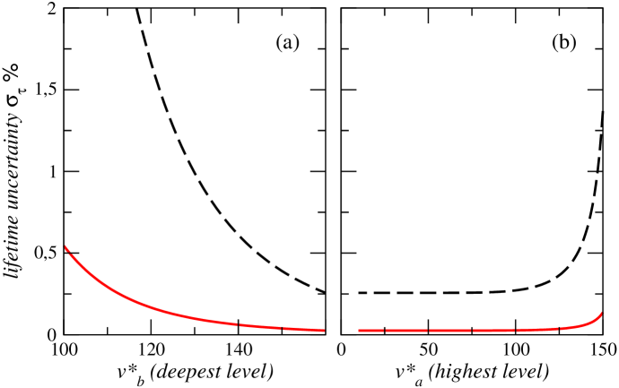
Figure 2: Variation of the relative uncertainty $\sigma_{\tau}$ on the lifetime value derived from an analysis using LeRoy-Bernstein law. The chosen example is the one of ⁸⁸Sr studied in Refs [20] and [16]. The experimental uncertainty on the level energy measurements is assumed to be $\sigma_{E}=300$ MHz (dashed lines) or $\sigma_{E}=30$ MHz (full lines). In the left graph, we show the variations of $\sigma_{\tau}$ vs the $v^{*}$ value of the deepest level included in the fit, $v^{*}_{b}$; the $v^{*}$ value of the highest level is kept constant at $v^{*}_{a}=10$. In the right graph, the roles of $v^{*}_{a}$ and $v^{*}_{b}$ are exchanged; the fixed value is $v^{*}_{b}=160$. It is of course assumed that the LeRoy-Bernstein law is valid down to this $v^{*}_{b}$ value.

It is interesting to notice that the present estimation of the error bar using the LeRoy-Bernstein law is meaningful for all studies of Section 4 (i.e. all studies but the $0_{g}^{-}$ ones), even if the analysis relies on quantum calculations. For calcium, using the $v^{*}$ values and the $\sigma_{E}$ value of Ref [19] we find $\sigma_{\tau}\sim 0.033~{}\%$ instead of $0.037~{}\%$; for strontium, using the $v^{*}$ values and the $\sigma_{E}$ value of Ref [20], we find $\sigma_{\tau}\sim 1.07~{}\%$ instead of $0.57~{}\%$. It is not surprising that the LR-B estimation gives a good result: as only two parameters are included in the fit, the situation is the same as in a LeRoy-Bernstein analysis. In the lithium studies, using the $v^{*}$ values of Ref [18] and assuming $\sigma_{E}\sim 100$ MHz gives $\sigma_{\tau}\sim 0.025~{}\%$ for ⁶Li and $\sigma_{\tau}\sim 0.11~{}\%$ for ⁷Li, instead of $\sigma_{\tau}\sim 0.026~{}\%$ for the two isotopes in the above reference. We did not expect such a good agreement, since three parameters are introduced in the model; it appears that the correlations between the $C_{3}$ and $C_{6}$ parameters (which are not included in our estimation) do not increase the uncertainty on the $C_{3}$ value.

5.3 Other cases

When the number of parameters increases, the matrix of the derivatives generally does not have a simple analytical expression. In the different studies of PAS on alkalis reviewed here, it is often difficult to retrieve how the different authors evaluate the given final error bar. The experimental uncertainty $\sigma_{E}$ is sometimes missing as well as the $\chi^{2}$ or $rms$ value characterizing their best fit and the corresponding residuals.

In the sodium case, we did not find the $\chi^{2}$ or $rms$ value of the fit (it could be recalculated, since calculated and measured values of the 7 vibrational levels are displayed), and neither the method used for the estimation of the uncertainty. Systematic errors coming from non-optimized parameters or from insufficiencies of the model were examined.

In the potassium case, the situation is similar. The $\chi^{2}$ value given in Table 2, 0.42, is derived from the $rms$ value of fit, 1.3x10^-3 cm^-1. Systematic errors are introduced, but it is difficult to find out wether the correlations between the 2 parameters are taken into account or not.

Concerning the first rubidium study [13], the $\chi^{2}$ value given in the Table, 2.5, has been recalculated to fit the definition of Equation (24) and might be considered as being a little too large. The estimation of the error bar on the final $C_{3}$ value is well described. Systematic errors are checked and correlations between parameters are in principle accounted for since the author draws the contours of the $\chi^{2}$ function just as described above (end of Section 5.1). However, we remark that some free parameters did not move (or moved extremely little) from their initial value. We observed a very similar situation in our work on cesium [10]: we attribute this pathological behavior to an overly large number of parameters, which are thus strongly correlated.

In the second study on rubidium [14], where the $rms$ value corresponds to a very satisfying $\chi^{2}$ value of 1.1, the evaluation of the uncertainty takes into account only the binary correlations between the parameters: the final error bar was therefore certainly underestimated.

Concerning cesium, the uncertainty obtained in the first paper [15] is one hundred times smaller than the one obtained in Ref [10], whereas the $rms$ value was notably smaller in the second paper. The bias introduced in the model by the omission of the two deepest levels can partially explain this somehow paradoxical situation. A slightly ”wrong” model requires more adjustable parameters, with more restrained values, leading to worse agreement between the data. In addition, in Ref [15] like in Ref [14], only binary correlations between the parameters were considered. In the second paper [10], we did a careful analysis of the estimation of the uncertainty of the lifetime value. What clearly appeared was that the interdependence of the parameters was very strong, probably because the number of parameters was too large. The $\chi^{2}$ value is rather small, which might be a clue to such a situation. We tried to linearize the model and to calculate the standard errors from the covariance matrix, as described above: the values obtained in this way were much too large for the linear approximation to remain valid. We thus tried to draw the contours of the $\chi^{2}$ function, but we found that the results of the fitting procedure depended in an unpredictable way on the allowed variation range of the parameters. Like in Ref [13], some free parameters did sometimes not move very much from their initial value. The consequence was that noticeably different parameter sets were yielding the same theory-experiment agreement. As available theoretical values of the long-range interaction coefficients are not precise enough, it is difficult to reduce the number of parameters of the fit. Reducing the experimental uncertainty $\sigma_{E}$ should probably allow one to get rid of these difficulties and would certainly increase the accuracy of the lifetime determination.

The difficulties one might encounter in the evaluation of the uncertainty as the number of parameters of the model increases is certainly no reason to give up on the determination of atomic radiative lifetime values through PAS: the conclusion of this section is that a careful analysis of the errors coming from the fit itself must always be performed, and that such a study will guide one in the choice of the model and of the energy range of the levels introduced in the fit.

6 Conclusion

In this paper we have reviewed recent experiments which derive atomic radiative lifetime values from photoassociative spectroscopy. This is possible because the energy spacing of the high-lying molecular states depends mainly on the long-range interatomic interaction, which itself depends on the same atomic radial integral as the atomic lifetime. Accurate values of atomic radiative lifetimes have always been difficult to obtain, both theoretically and experimentally. The emergence of the PAS method of determination, based on a conceptually new approach, is thus very interesting. As potential systematic errors are quite different from those expected in atomic physics experiments, for instance, it provides a useful check on these lifetime determinations. The lifetime values discussed in this paper are summarized in Figure 3, where the high quality of the PAS data is clearly visible.

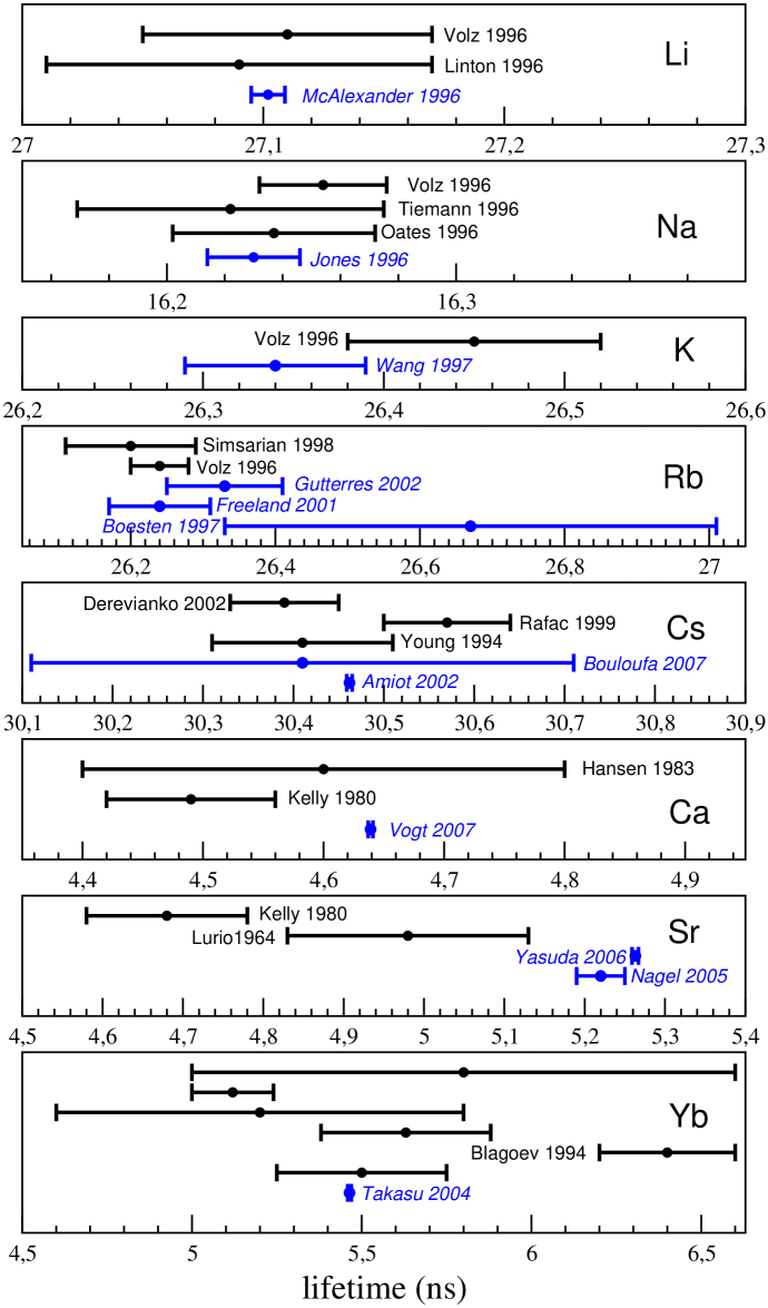
Figure 3: Summary of the radiative lifetime values for all elements discussed in the present work. The names of authors using photoassociation spectroscopy are displayed in italics. For ytterbium, all reported values but the PAS one are extracted from the review of Blagoev and Komarovskii [58].

The analysis consists in extracting, from the spectroscopic data, a precise long-range coefficient: a model is chosen for the calculation of the level energies and the parameters of the model are fitted to the experimental data. The model is either semi-classical or quantum-mechanical. In the first case, a two-parameter model, the so-called LeRoy-Bernstein law, was used in Sr and Yb studies. Otherwise, molecular potentials have to be considered. In principle, the long-range interaction has to be connected with ab initio or RKR potentials, as was the case for the Li, Ca and Sr studies. In the case of Na, K, Rb and Cs, the relevant potentials are called ”pure long-range” and involve only long-range interaction parameters. The $R^{-3}$ behavior of the long-range interaction which is the basis of the lifetime determination is only asymptotically valid. A number of effects, which are likely to contribute to the interaction energy, have been introduced in the models, at the cost of an increased number of parameters.

Concerning the LeRoy-Bernstein approach, we first recall that its validity should always be carefully checked. Concerning the precision that can then be obtained, a very simple calculation allows one to predict the uncertainty on the lifetime value starting from the experimental value of the spectroscopic uncertainty and from the $v$ values of the vibrational levels introduced in the fit. The predictions are the same for quantum calculations as long as only two free parameters are needed. When additional parameters are introduced, the estimation of the uncertainty is more difficult. It has probably been sometimes underestimated, mainly because the role of the correlations between the parameters was not wholly considered. We recall a simple and general estimation of these effects, based on a linearization of the model. If it is not possible to apply it, contour calculations of the $\chi^{2}$ function have to be drawn and one has to carefully check the reproducibility of the convergence process: in the cesium case, for instance, we observed unpredictable results, due to an overly large number of parameters. We hope to solve this particular problem with the analysis of new experimental PAS results with improved accuracy currently in progress in our lab.

In spite of these difficulties, the ensemble of atomic radiative lifetimes results obtained through PAS is quite impressive and convincing. A number of accurate values have been derived, and they agree well with most of the previous results, obtained from accurate atomic physics measurements [8]. The agreement with available theoretical results is generally satisfying. It is even excellent in the case of lithium for which very precise calculations have been performed due to its simple atomic structure.

Finally, the PAS method for extracting accurate atomic radiative lifetimes could represent a promising perspective for other elements which are nowadays laser-cooled and trapped, like Magnesium [74], Chromium [75], Silver [76], Erbium [77], Francium [78], and Radium [79], provided that trapping densities are high enough to perform efficient PA experiments.

References

References

- [1] Jönsson P, Ynnerman A, Fischer C F, Godefroid M R and Olsen J 1996 Phys. Rev. A 53 4021
- [2] Porsev S G, Kozlov M G, Rakhlina Y G and Derevianko A 2001 Phys. Rev. Lett. 64 012508
- [3] Fischer C F and Tachiev G 2003 Phys. Rev. A 68 012507
- [4] Bennett S C and Wieman C E 1999 Phys. Rev. Lett. 82 2484
- [5] Guena J, Lintz M and Bouchiat M A 2005 Phys. Rev. A 71 042108
- [6] Derevianko A and Porsev S G 2007 Eur. Phys. J. A 32 517
- [7] Regan B C, Commins E D, Schmidt C J and DeMille D 2002 Phys. Rev. Lett. 88 071805
- [8] Volz U and Schmoranzer H 1996 Physica Scripta T65 48
- [9] McAlexander W I, Abraham E R I and Hulet R G 1995 Phys. Rev. A 51 R871
- [10] Bouloufa N, Crubellier A and Dulieu O 2007 Phys. Rev. A 75 052501
- [11] Jones K M, Julienne P S, Lett P D, Phillips W D, Tiesinga E and Williams C J 1996 Europhys. Lett. 35 85
- [12] Wang H, Li J, Wang X, Williams C, Gould P L and Stwalley W 1997 Phys. Rev. A 55 R1569
- [13] Freeland R S 2001 Photoassociation Spetroscopy of ultracold and Bose-Condensed Atomic Gasses Ph.D. thesis university of Texas at Austin
- [14] Gutterres R, Amiot C, Fioretti A, Gabbanini C, Mazzoni M and Dulieu O 2002 Phys. Rev. A 66 024502
- [15] Amiot C, Dulieu O, Gutterres R F and Masnou-Seeuws F 2002 Phys. Rev. A 66 052506
- [16] Yasuda M, Kishimoto T, Takamoto M and Katori H 2006 Phys. Rev. A 73 011403
- [17] Takasu Y, Komori K, Honda K, Kumakura M, Yabuzaki T and Takahashi Y 2004 Phys. Rev. Lett. 93 123202
- [18] McAlexander W I, Abraham E R I and Hulet R G 1996 Phys. Rev. A 54 R5
- [19] Vogt F, Grain C, Nazarova T, Sterr U, Riehle F, Lisdat C and Tiemann E 2007 Eur. Phys. J. D 44 73
- [20] Nagel S B, Mickelson P G, Saenz A D, Martinez Y N, Chen Y C, Killian T C, Pellegrini P and Côté R 2005 Phys. Rev. Lett. 94 083004
- [21] Pichler G, Milosevic S, Veza D and Beuc R 1983 J. Phys. B: Atomic Molecular and Optical Physics 16 4619
- [22] Jones R B, Schloss J H and Eden J G 1993 J. Chem. Phys. 98 4317
- [23] Marvet U and Dantus M 1995 Chem. Phys. Lett. 245 393
- [24] Ban T, Ter-Avetisyan S, Beuc R, Skenderovic H and Pichler G 1999 Chem. Phys. Lett. 313 110
- [25] Thorsheim H R, Weiner J and Julienne P S 1987 Phys. Rev. Lett. 58 2420
- [26] Lett P D, Helmerson K, Philips W D, Ratliff L P, Rolston S L and Wagshul M E 1993 Phys. Rev. Lett. 71 2200
- [27] Miller J D, Cline R A and Heinzen D J 1993 Phys. Rev. Lett. 71 2204
- [28] Stwalley W and Wang H 1999 J. Molec. Spect. 195 194
- [29] Jones K M, Tiesinga E, Lett P D and Julienne P S 2006 Rev. Mod. Phys. 78 483
- [30] Evseev A V, Radtsig A A and and B M S 1978 Optics Spectrosc. 44 495
- [31] Marinescu M and Dalgarno A 1996 Z. Phys.D 36 239
- [32] Casimir H B G and Polder D 1948 Phys. Rev. 73 360
- [33] McLone R and Power E 1965 Mathematika 11 91
- [34] Meath W J 1968 J. Chem. Phys. 48 227
- [35] Aymar M, Dulieu O and Spiegelmann F 2006 Eur. Phys. J. D 39 S905
- [36] Bunker P R 1968 J. Molec. Spect. 28 422
- [37] LeRoy R J and Bernstein R B 1970 J. Chem. Phys. 52 3869
- [38] Stwalley W C, Uang Y H and Pichler G 1978 Phys. Rev. Lett. 41 1164
- [39] Dashevskaya E I, Voronin A I and Nikitin E E 1969 Can. J. Phys. 47 1237
- [40] Movre M and Pichler G 1977 J. Phys. B: Atomic Molecular and Optical Physics 10 2631
- [41] Boesten H M J M, Tsai C C, Gardner J R, Heinzen D and Verhaar B J 1997 Phys. Rev. A 55 636
- [42] Derevianko A and Porsev S G 2002 Phys. Rev. A 65 053403
- [43] Chin C, Vuletic V, Kerman A J, Chu S, Tiesinga E, Leo P J and Williams C J 2004 Phys. Rev. A 70 032701
- [44] Oates C W, Vogel K R and Hall J L 1996 Phys. Rev. Lett. 76 2866
- [45] Tiemann E, Kn ckel H and Richling H 1996 Z. Phys.D 37 323
- [46] Simsarian J E, Orozco L A, Sprouse G D and Zhao W Z 1998 Phys. Rev. A 57 2448
- [47] Young L, III W H, Sibener S, Price S, CETanner, Wieman C and Leone S R 1994 Phys. Rev. A 50 2174
- [48] Rafac R J, Tanner C E, Livingston A E, Berry K W K H G and Kurtz C A 1999 Phys. Rev. A 60 3648
- [49] Fioretti A, Amiot C, Dion C M, Dulieu O, Mazzoni M, Smirne G and Gabbanini C 2001 Eur. Phys. J. D 15 189
- [50] Fioretti A, Comparat D, Drag C, Amiot C, ODulieu, Masnou-Seeuws F and Pillet P 1999 Eur. Phys. J. D 5 389
- [51] Marinescu M and Dalgarno A 1995 Phys. Rev. A 52 311
- [52] Gabbanini C, Fioretti A, Lucchesini A, Gozzini S and Mazzoni M 2000 Phys. Rev. Lett. 84 2814
- [53] Drag C, Tolra B L, Dulieu O, Comparat D, Vatasescu M, Boussen S, Guibal S, Crubellier A and Pillet P 2000 IEEE J. Quant. Electron. 36 1378
- [54] Ji B, Tsai C C and Stwalley W C 1995 Chem. Phys. Lett. 206 103
- [55] Vatasescu M, Dulieu O, Amiot C, Comparat D, Drag C, Kokoouline V, Masnou-Seeuws F and Pillet P 2000 Phys. Rev. A 61 044701
- [56] Comparat D 2004 J. Chem. Phys. 120 1318
- [57] Jelassi H, Viaris de Lesegno B, Pruvost L 2008 submitted to Phys. Rev. A
- [58] Blagoev K B and Komarovskii V A 1994 AT. Data Nucl. Data Tab. 56 1
- [59] Linton C, Martin F, Russier I, Ross A J, Crozet P, Churassy S and Bacis R 1996 J. Molec. Spect. 175 340
- [60] Hansen W 1983 J. Phys. B: Atomic Molecular and Optical Physics 16 2309
- [61] Kelly F M and Arthur M S 1980 Can. J. Phys. 58 1416
- [62] Lurio A, deZafra R L and Goshen R J 1964 Phys. Rev. 134 A1198
- [63] Yan Z C and Drake G W F 1995 Phys. Rev. A 52 R4316
- [64] Bohn J L and Julienne P S 1999 Phys. Rev. A 60 414
- [65] Allard O, Samuelis C, Pashov A, Knöckel H and Tiemann E 2003 Eur. Phys. J. D 26 155
- [66] Crubellier A, Dulieu O, Masnou-Seeuws F, Elbs M, Knöckel H and Tiemann E 1999 Eur. Phys. J. D 6 211
- [67] Vanhaecke N, Lisdat C, T’Jampens B, Comparat D, Crubellier A and Pillet P 2004 Eur. Phys. J. D 28 351
- [68] Allard O 2004 Long-range interactions in the calcium dimer studied by molecular spectroscopy Ph.D. thesis Universität Hannover
- [69] Bussery-Honvault B and Moszynski R 2006 Mol. Phys. 104 2387
- [70] Boutassetta N, Allouche A R and Aubert-Frécon M 1996 Phys. Rev. A 53 3845
- [71] Féménias J L 2003 J. Molec. Spect. 217 32
- [72] Vanhaecke N 2003 Molecules froides: formation, piegeage et spectroscopie Ph.D. thesis Université Paris-Sud, Orsay
- [73] Particle Data Group 2000 Eur. Phys. J. C 15 1
- [74] Sengstock K, Sterr U, Müller J H, Rieger V, Bettermann D and Ertmer W 1994 Appl. Phys. B 59 99
- [75] Bell A S, Stuhler J, Locher S, Hensler S, Mlynek J and Pfau T 1999 Europhys. Lett. 45 156
- [76] Uhlenberg G, Dirscherl J and Walther H 2000 Phys. Rev. A 62 063404
- [77] Berglund A J, Lee S A and McClelland J J 2007 Phys. Rev. A 76 053418
- [78] Sprouse G D, Orozco L A, Simsarian J E and Zhao W Z 1998 Nucl. Phys. A 630 316
- [79] Guest J R, Scielzo N D, Ahmad I, Bailey K, Greene J P, Holt R J, Lu Z T, Connor T P O and Potterveld D H 2007 arXiv physics/0701263v3