Mapping the magnetosphere of PSR B1055–52

Abstract

We present a geometric study of the radio and $\gamma$-ray pulsar B1055–52 based on recent observations at the Parkes radio telescope. We conclude that the pulsar’s magnetic axis is inclined at an angle of $75^{\circ}$ to its rotation axis and that both its radio main pulse and interpulse are emitted at the same height above their respective poles. This height is unlikely to be higher or much lower than 700 km, a typical value for radio pulsars.

It is argued that the radio interpulse arises from emission formed on open fieldlines close to the magnetic axis which do not pass through the magnetosphere’s null (zero-charge) surface. However the main pulse emission must originate from fieldlines lying well outside the polar cap boundary beyond the null surface, and farther away from the magnetic axis than those of the outergap region where the single $\gamma$-ray peak is generated. This casts doubt on the common assumption that all pulsars have closed, quiescent, corotating regions stretching to the light cylinder.

Figure 1: The pulse profile of the 1369 MHz timing data of PSR B1055–52 at 20 cm showing total intensity (solid line), linear polarization (dashed line) and circular polarization (dotted line).

1 Introduction

PSR B1055–52 is a middle-aged (0.5 Myr) energetic ($\dot{E}=3\times 10^{34}$ erg s^-1) pulsar which has been detected as a source of pulsed $\gamma$-rays. In their study of energetic pulsars, Weltevrede & Johnston (2008) singled out PSR B1055–52 for comment since it is exceptional in having both an interpulse and wide radio components, with the interpulse (IP) well separated from the main pulse (MP). In general the presence of an IP is a strong clue to a pulsar’s geometry, and suggests that a study of the radio emission of PSR B1055–52 may give insight into the structure of the magnetosphere and the origin of its $\gamma$-rays.

PSR B1055–52 was discovered with the Molongolo telescope by Vaughan & Large (1972), who noted a possible IP in one of their records. The IP was confirmed by McCulloch et al. (1976), who commented that the pulse profile resembles that of the Crab pulsar. Rankin (1983) noted that the MP-IP separation shows no variation with frequency, which is additional evidence that the pulsar’s magnetic axis is highly inclined to the rotation axis. Lyne & Manchester (1988) concluded that the observed polarisation position angle (PA) swings of the MP and IP suggest an angle of inclination of the magnetic axis of $75^{\circ}$, without ruling out higher values around $90^{\circ}$. This general view was supported in a complex study published by Biggs (1990a).

PSR B1055–52 is relatively close, which makes it possible to observe its emission over a wide range of wavelengths. The pulsar’s $DM$ distance is only $0.72\pm 0.2$ kpc (Cordes & Lazio, 2002), roughly consistent with the X-ray data (e.g. Ögelman & Finley 1993) and the non-thermal radio source around PSR B1055–52 (Combi et al. 1997).

The EGRET detector (Energetic Gamma-Ray Experiment Telescope) on board of the Compton Gamma Ray Observatory (CGRO) revealed that PSR B1055–52 is a pulsed $\gamma$-ray source (Thompson et al. 1999). Unlike most $\gamma$-ray profiles (but in common with PSR B1706–44), that of PSR B1055–52 does not show two narrow peaks separated by 0.4–0.5 in phase, but has a broad $\gamma$-ray profile with possible sub-peaks at the leading and trailing edge of the profile which peak 0.25 and 0.05 in phase before the radio MP (Thompson et al., 1999). The leading side of the profile has also been seen with the COMPTEL detector (0.75–30 MeV), while only the trailing side of the profile is seen above 2 GeV by EGRET, suggesting a longitude dependent spectral index.

Another feature which makes PSR B1055–52 an interesting source at high energies is its spin-down age of 0.5 Myr, making PSR B1055–52 (at the time of writing) the oldest of the known $\gamma$-ray pulsars. Its period of 0.197 seconds makes it also the slowest (excluding Geminga). This status as being both an ‘old’ young pulsar and, at the same time a ‘young’ old pulsar (most radio pulsars are over 1 Myr old) suggests that it may possess characteristics of both and give insight into the link between high-energy production in the outer magnetosphere and radio emission above the polar cap. It has famously been dubbed as one of the ‘Three Musketeers’ (Becker & Trümper, 1997), along with PSR B0656+14 and Geminga, because these pulsars were found to emit solely thermal X-rays which are interpreted as the product of initial neutron star cooling.

The geometry linking the high-energy and radio profiles was recently studied by Wang et al. (2006), who made use of the PA analysis of Lyne & Manchester 1988. They concluded that that the radio MP and IP are emitted from separate poles with the $\gamma$-ray emission coming from the same pole as the radio MP. They claim that the IP and MP come from different heights, but do not consider the effect of retardation and aberration on the PA-curve. In their model the radio emission occurs on fieldlines which are confined to a polar cap bounded by the last closed fieldlines which, in a dipole geometry, touch the light cylinder. Here we use new data to re-analyse the PA-swings and to create a geometry which is fully consistent with retardation and aberrational effects. A full understanding of the geometry is an important prelude to undertaking an analysis of the pulsar’s complex single pulse behaviour, which will appear in a subsequent paper.

The organisation of this paper is as follows: in Sect. 2 details about the radio data used are provided, in Sect. 3 the properties of the pulse profile of PSR B1055–52 are described and its most likely geometry is derived in Sect. 4. In Sect. 5 we identify the active fieldlines of the MP and IP and the implications of our results are discussed in Sect. 6.

2 Observations

The pulse profile of PSR B1055–52 was obtained at three different frequencies by the Parkes 64-m radio telescope located in Australia. During an observing session carried out from 2006 August 24 to 27 data was recorded using the H-OH receiver (1369 MHz centre frequency, 256 MHz bandwidth split into 1024 frequency channels with an equivalent system flux density of 43 Jy; Johnston 2002) and the 10/50 cm receiver (3094/653 MHz centre frequency, 1024/64 MHz bandwidth split into 1024/512 frequency channels with an equivalent system flux density of 49/57 Jy on a cold sky). The signals from the two linear feeds of the receiver were converted into Stokes parameters, resampled and folded at the pulse period by a digital filterbank using 512 bins across the profile. In addition we also used the pulse profile with a slightly higher time resolution (1024 bins across the profile) obtained using the 20 cm multibeam receiver (1369 MHz centre frequency, 256 MHz bandwidth split into 1024 frequency channels with an equivalent system flux density of 35 Jy on a cold sky) for the Fermi timing program. This program started in April 2007 with the aim to provide timing solutions which can be used to fold $\gamma$-ray data obtained by the Fermi satellite (Smith et al., 2008). The profile is the sum of 33 individual observations with a total length of 6.6 hours. For details about the data-processing we refer to Weltevrede & Johnston (2008).

3 Pulse profile

3.1 Profile morphology

The shape of the pulse profile of PSR B1055–52 is quite complex, as one can see in Fig. 1. In a similar way to Biggs (1990a) (who did not detect the first component of the MP), we call the four most prominent peaks of the MP peaks I to IV and the three peaks in the IP V to VII. Long integrations are required to obtain stable profiles, with evidence for persistent intensity changes in component III (also noted by Biggs 1990a). The peak-to-peak separation between the MP and IP is $\sim 159^{\circ}$, well below $180^{\circ}$, so it is not immediately obvious that we are dealing with emission from both poles of the neutron star.

As one can see in Fig. 1, the profile of the MP is highly linearly polarized. This is also the case for the leading edge of the IP, but at later pulse longitudes it becomes almost completely depolarized (e.g. McCulloch et al. 1978). Notice that all three components of the IP have a distinct linear polarization peak, although they are much weaker for components VI and VII (Fig. 1). The profiles of the degree of linear polarization at 10 cm and 50 cm (not shown) look very similar to that at 20 cm.

Component II of the MP has a significant amount of circular polarization, although it is weak. There is a hint that the trailing part IP also has a significant amount of circular polarization, but with an opposite sign.

3.2 Frequency evolution of the pulse profile

Figure 2: Top panels: The pulse profiles of PSR B1055–52 at three observing frequencies drawn with different vertical offsets. From top to bottom the wavelength are 10 cm, 20 cm and 50 cm. Bottom panels: The PA of the linear polarization and an RVM fit. The offsets are the same as in the top panels. These are the August 2006 observations.

The pulse profiles of PSR B1055–52 at different frequencies are shown in Fig. 2. The profiles are aligned and normalized using the peak of component II which is put at $90^{\circ}$ pulse longitude. One can see that there is not much evidence for frequency evolution in the relative position of the components, but the peak amplitudes do evolve with frequency. In the MP the first component disappears at 50 cm while components III and IV become relatively stronger. The IP shows a similar frequency evolution with the leading half of the profile becoming weaker relative to the trailing component. In relative terms, the IP itself is strongest at high frequencies. While the components of the IP are sharper at 10 cm this is less clear in the MP. Notice also that component VII is the only component which changes its centroid position with respect to the other components.

There is also no evidence of the full widths of the MP and IP (or their separation) being frequency-dependent, potentially an important hint as to the pulsar’s geometry. A profile at 170 MHz, ascribed to McCulloch et al. and published in Rankin (1983), shows a merging of components III and IV in the MP, but little overall widening of the profiles.

4 Geometric implications

The PA-swing is plotted in the bottom panel of Fig. 2 for the three frequencies. We found a significant offset of the 50 cm data with respect to the other wavelengths when we use the rotation measure (RM) of $47.2\pm 0.8$ rad m^-2 (Taylor et al., 1993). By applying an RM of 46 rad m^-2 the PA-swings at the different frequencies line up, suggesting that the shape of the PA-swing, like that of the profile, is independent of frequency. This value of the RM is consistent with the value of $44\pm 2$ rad m^-2 measured by Noutsos et al. (2008).

The shape of the PA-swing can be used to constrain the angles between the magnetic and rotation axis ($\alpha$) and the angle between the line of sight and the rotation axis ($\zeta=\alpha+\beta$, where $\beta$ is the impact parameter). According to the rotating vector model (RVM; Radhakrishnan & Cooke 1969) the PA ($\psi$) can be described as a function of the pulse longitude $\left(\phi\right)$ by

$$\tan\left(\psi-\psi_{0}\right)=\frac{\sin\alpha\;\sin\left(\phi-\phi_{0}\right)}{\sin\zeta\;\cos\alpha-\cos\zeta\;\sin\alpha\;\cos\left(\phi-\phi_{0}\right)},$$ (1)

where $\psi_{0}$ and $\phi_{0}$ are the PA and the pulse longitude corresponding to the inflection point of the PA-swing. Using this definition implies that we follow the observer’s sign convention for the PA, which differs from that introduced by Damour & Taylor (1992) and Everett & Weisberg (2001).

If the emission height $r$ is zero, or at least negligible compared with the light cylinder radius $R_{LC}$, the inflection point of the PA-swing coincides with the fiducial point (defined as the pulse longitude where the magnetic pole at the surface is directed towards us). However, for non-zero emission heights this is no longer the case. As the emission height increases the total intensity appears to shift towards earlier pulse longitudes due to aberration (by $r/R_{LC}$) and the decreasing light travel distance to the observer (also by $r/R_{LC}$), while the PA-swing shifts to later pulse longitudes with respect to the fiducial point (by $2r/R_{LC}$). Thus the total relative shift between the steepest gradient of the PA-swing with respect to the emission beam’s centroid is given by

$$\Delta\phi_{\mathrm{BCW}}=4r/R_{LC}$$ (2)

(Blaskiewicz et al. 1991; Dyks 2008), where $r$ is assumed to be small compared with $R_{LC}$.

In PSR B1055–52 the degree of linear polarization is low in the trailing half of the IP, but fortunately it is enough to obtain the PA. This means we have a full PA coverage at virtually every pulse longitude where emission is detected at a far better time resolution than was available to Lyne & Manchester (1988). This enables us to re-examine and place constraints on the geometric solution of this pulsar. In this section we formally confirm that a nearly-orthogonal solution is preferable to a nearly-aligned solution and exploit the $\gamma$-ray profile to establish an integrated geometry.

4.1 Nearly-aligned rotator?

We first consider the possibility that PSR B1055–52 might be a nearly-aligned rotator. In such a geometry the MP and IP originate from the two edges of a hollow cone-like beam from a single pole (e.g. Manchester & Lyne 1977). The separation between the two components can be large, but, as observed, will not necessarily be $180^{\circ}$ in pulse longitude. The large widths of the components together with the steep trailing edge of the MP and the leading edge of IP are also typical for such geometry, making this model a promising possibility to consider.

However, for a nearly-aligned rotator one expects the PA-swing to be flatter than is observed. In the RVM model the steepest gradient is associated with the line of sight passing the fiducial plane. In the case of an aligned rotator this plane should be at a pulse longitude between the MP and IP, hence the observed PA-swing will be relatively flat. As has been pointed out (by Wang et al. 2006 for example), the steepness of the PA-swing observed for both the MP and IP rules out the one pole geometry. It should be added that this conclusion is also valid even when $90^{\circ}$ jumps in the PA-swing caused by different plasma modes dominating in different parts of the pulse profile (e.g. Manchester et al. 1975) are considered.

The PA-swing inflection point can in principle be shifted from its unshifted pulse longitude between the MP and IP (as would be expected for an aligned rotator) to appear at the pulse longitude of one of the pulse components (MP or IP) when the aberrational shift of Eq. 2 is considered. This effect could therefore in principle make the PA-swing steep in one of the two components. However, it cannot make them steep in both since the RVM model predicts a steep gradient at only one point in the PA-curve, thereby failing to explain the observed PA-swing.

4.2 Nearly orthogonal rotator

Figure 3: The reduced $\chi^{2}$ grid obtained by fitting the RVM to the PA-swing of both the MP and IP of the 1369 MHz timing data. Black corresponds to 2.7 and white to 20. The cross indicates the position of the minimum of the $\chi^{2}$ surface ($\alpha_{\mathrm{MP}}=75^{\circ}$ and $\beta_{\mathrm{MP}}=36.1^{\circ}$). Solutions to the right of the right hand side diagonal solid line are excluded because they require a $\beta_{\mathrm{IP}}>90^{\circ}$ and solutions to the left of the left hand side diagonal solid line are excluded because they require a negative $\beta_{\mathrm{IP}}$ (corresponding to a declining PA-swing for the IP). Solutions below the dashed line (for $\alpha_{\mathrm{MP}}<90^{\circ}$) and above the dashed line (for $\alpha_{\mathrm{MP}}>90^{\circ}$) are excluded as they do not allow the $\gamma$-ray emission to be emitted from above the null line.

In searching for a self-consistent solution, we follow Wang et al. (2006) and consider a model where the profile of PSR B1055–52 is generated by emission from an orthogonal rotator.

Although McCulloch et al. (1978) claimed that the PA-swing cannot be extrapolated between the MP and IP, we (like Wang et al. 2006 with inferred data from Lyne & Manchester 1988) had no problem in fitting the PA-curve with the RVM model (Eq. 1). In fact, the reduced $\chi^{2}$ of 2.7 is quite good, although not perfect (Fig. 3). The lowest $\chi^{2}$ is found for $\alpha_{\mathrm{MP}}=75^{\circ}$ and $\beta_{\mathrm{MP}}=36.1^{\circ}$ (where $\alpha_{\mathrm{MP}}$ and $\beta_{\mathrm{MP}}$ are the MP values of $\alpha$ and $\beta$), suggesting that the orientation of the magnetic axis is indeed close to orthogonal and in agreement with Wang et al. (2006). This implies $\alpha_{\mathrm{IP}}=180^{\circ}-\alpha_{\mathrm{MP}}=105^{\circ}$ and an impact parameter at the IP of $\beta_{\mathrm{IP}}=\beta_{\mathrm{MP}}+2\alpha_{\mathrm{MP}}-180^{\circ}=6.1^{\circ}$. Note that these fits require that all the emission at each pole comes from the same height, a point to which we will return in Sect. 5.2. The best fit is shown in Fig. 2 as the solid curve. The biggest discrepancy between the fit and the data occurs in the trailing component of the IP, where the fit is too flat compared with the model. The steepest gradient in the MP ($\phi_{0}$ of Eq. 1) is found exactly at the location of the highest peak in the pulse profile ($\phi=90^{\circ}$ in the plots).

The fact that the PA-swing can be extrapolated between the MP and IP further implies that the emission heights at both poles cannot be too large. If there were a large differential emission height, the PA-swings of the MP and IP would be shifted by different amounts (Blaskiewicz et al. 1991; Hibschman & Arons 2001; Dyks 2008), making it impossible to fit the PA-swing with a single RVM curve. By modelling these relative shifts we find that the lowest $\chi^{2}$ is found when the emission height of the IP is higher than that of the MP by $0.07R_{\mathrm{LC}}$ ($\approx{700}$ km) with an uncertainty of $0.10R_{\mathrm{LC}}$ ($\approx{1000}$ km), which is consistent with the emission height being identical at both poles. The uncertainty is derived by finding the differential emission height at which the reduced $\chi^{2}$ of the PA fit has doubled. Although the solution found by Wang et al. (2006) (who find an IP/MP emission height differential of between $0.10R_{\mathrm{LC}}$ and $0.20R_{\mathrm{LC}}$) is in the allowed range, we will argue later that this solution is very unlikely. We therefore seek a solution with identical emission heights for the MP and IP.

4.3 Implications of the $\gamma$-ray profile

As Lyne & Manchester (1988) pointed out, and as is evident in Fig. 3, there are RVM solutions over a wide range of $\alpha_{\mathrm{MP}}$ values which have a comparable $\chi^{2}$. However, we can utilize additional constraints to confirm that we have the right solution. By assuming that $\beta_{\mathrm{IP}}$ must be smaller than $90^{\circ}$ (or else the full opening angle of the radio beam would be larger than $180^{\circ}$) and that $\beta_{\mathrm{IP}}$ must be positive (or else the PA-swing of the IP would decrease) only solutions between the two diagonal solid lines in Fig. 3 are allowed.

A further and critical constraint can come from the observed phase and width of the $\gamma$-ray profile (Thompson et al. 1999). Different magnetospheric locations are proposed for the $\gamma$-ray emission of pulsars. Early models put the acceleration zones at low altitudes above the magnetic poles (polar cap models; e.g. Daugherty & Harding 1996). More recently, it has been argued that the emission height could be considerably larger for fieldlines close to the last open fieldlines giving rise to the “slot gap” model (e.g. Muslimov & Harding 2004a) and the “two-pole caustic” model (Dyks & Rudak, 2003). A separate class of models are the so-called “outergap” models (Cheng et al., 1986; Romani, 1996), which place the acceleration zones above the “null lines” (Holloway, 1973). These are the lines on which the charge density of a pulsar magnetosphere changes sign (Goldreich & Julian 1969).

Numerical simulations show that only an outer gap model can reproduce the observed shape of the $\gamma$-profile of PSR B1055–52 to a good approximation (Watters et al., 2008). The two-pole caustic model, which has $\gamma$-ray production below the null line, predicts in general profiles with observed emission from both magnetic poles, which makes it difficult to reproduce the observed $\gamma$-ray pulse width. In order to reproduce the observed single-peaked $\gamma$-ray profile the two-pole caustic model predicts either $\alpha$ or $\zeta$ values smaller than allowed by the PA-swing parameters between the two solid diagonal lines of Fig. 3. Polar cap models, which have low emission heights, also require too small $\alpha$ and $\zeta$ values in order to get a broad enough $\gamma$-ray profile. On the other hand outer gap models predict, by definition, that only emission from one pole can be seen for any given observer, thereby qualitatively reproducing the observed $\gamma$-ray profile for a wide range of geometries.

In order to reproduce the observed width of the $\gamma$-ray profile the gap thickness $w$ (the fraction of the angle from the last closed fieldline to the magnetic axis) should be of the order of $0.18$ (assuming that the $\gamma$-ray efficiency is equal to $w$), showing that the gap is very large in comparison with most $\gamma$-ray pulsars (Watters et al., 2008). Large outer gaps are typical for highly efficient old $\gamma$-ray pulsars (e.g. Romani 1996). The outer gap model further predicts that two caustics are formed at the edges of the $\gamma$-ray beam, which could account for the sub-structure visible in the EGRET data.

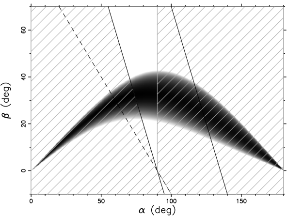
Figure 4: The reduced $\chi^{2}$ grid obtained by fitting only the PA of the 1369 MHz timing data of the MP region. Black corresponds to 1.1 and white to 3.0. For an explanation of the lines see Fig. 3.

If we accept that the $\gamma$-rays are produced above the null surface of the MP (i.e. they are produced by the outer gap) large parts of the $\alpha_{\mathrm{MP}}-\beta_{\mathrm{MP}}$ plane can be ruled out. Together with the $0^{\circ}<\beta_{IP}<90^{\circ}$ restriction we can eliminate the entire hashed regions in Fig. 3 from consideration. As one can see in Fig. 4, using these constrains the geometry of PSR B1055–52 is already constrained even without fitting the shape of the PA-swing of the IP as there is only a relatively small wedge shaped region of allowed solutions in the plot. This is important, because it shows that our conclusions do not depend strongly on the shape of the PA-swing of the IP which deviates slightly from the RVM prediction. We will therefore adopt the RVM solution with the lowest $\chi^{2}$ in this paper which has $\alpha_{\mathrm{MP}}=75^{\circ}$ and $\beta_{\mathrm{MP}}=36.1^{\circ}$.

4.4 The geometric picture

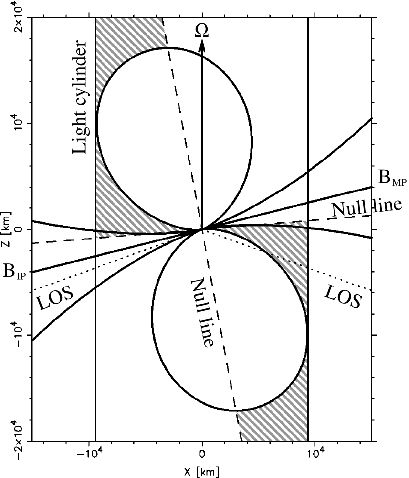
Figure 5: The geometry of the dipole field of PSR B1055–52 assuming $\alpha_{\mathrm{MP}}=75^{\circ}$. The rotation axis points upwards and the light cylinder is indicated by the vertical lines. The line of sight (dotted line “LOS”) makes a large angle ($36.1^{\circ}$) with the magnetic axis of the MP (right hand side of the plot), while this angle is much smaller ($6.1^{\circ}$) for the IP (left hand side of the plot). The dashed lines indicate the location of the null surface, and the last closed fieldlines which conventionally define a corotating region are shown. At the MP we must be viewing fieldlines which lie above the null surface (in the shaded region) – and which will be well within the corotating region if the radio emission is, as usually assumed, close to the surface. The $\gamma$-ray profile, which is observed to overlap the MP radio emission, is most likely formed in the shaded area, which indicates the volume above the null surface where an outer gap could potentially be formed.

The emission geometry in the fiducial plane is illustrated in Fig. 5. One can see that the line of sight passes the magnetic axis of the IP much more closely than to the pole of the MP, consistent with the steeper slope of the PA-swing of the IP. Thus, the IP emission must arise from open fieldlines as is generally thought to be the case for radio pulsars. However, the incidence of the line of sight with the magnetic axis of the MP is very large, which immediately leads to one of two possibilities. If we require the emission to arise from open fieldlines, then it must originate at a considerable fraction of the light cylinder. Otherwise we are forced to accept emission from presumed closed fieldlines at low altitudes.

Fig. 5 also shows the null lines (dashed). These are the $\mathbf{\Omega}\cdot\mathbf{B}=0$ lines on which the charge density of the magnetosphere changes sign. The tangent of the fieldlines are perpendicular to the rotation axis at the point where they intersect the null line. It immediately follows that for the assumed geometry we ‘see’ fieldlines above the null line for the MP (Fig. 5), which suggests that the radio MP is produced in a region where an outergap is likely to exist. It can be shown that this is a general rule. In any pulsar where emission from both poles are detected, at one of the poles our line of sight must see emission from the region above the null line, i.e. the likely site of any “outergap”. Assuming that this outergap is the site of the observed $\gamma$-ray emission, it is no surprise that the phase range of the $\gamma$-ray profile overlaps that of the MP rather than the IP. We note that were we to choose an RVM solution with $\alpha_{\mathrm{MP}}>90^{\circ}$, then the IP would be the pole which views the outergap region, and the $\gamma$-ray profile would be at the wrong phase.

Most other known $\gamma$-ray pulsars are, unlike PSR B1055–52, typically found to have a single peaked radio profile with a large offset from the $\gamma$-ray profile. The lines of sight of these pulsars are also believed to have a large $\beta$ value for one of the poles. This causes the line of sight to miss the radio beam of the magnetic pole for which the $\gamma$-rays are observed, hence a large offset is seen between the radio and the $\gamma$-rays. PSR B1055–52 is different because, for some reason, it has a large enough radio beam to be seen by a line of sight with a large angle $\beta$.

One further conclusion can also be drawn. With $\beta_{\mathrm{MP}}$ being so large at the MP ($36.1^{\circ}$), the corresponding $\beta_{\mathrm{IP}}$ at the IP will be positive (since $\beta_{\mathrm{IP}}=\beta_{\mathrm{MP}}+2\alpha_{\mathrm{MP}}-180^{\circ}=6.1^{\circ}$). This implies that at the IP we view the pole on the side away from the null line, and therefore do not see fieldlines which thread the outergap region.

5 Beam illumination

5.1 Beam mapping

We now use the widths of the MP and IP pulse profile to place additional constraints on the magnetosphere’s geometry. The first point that needs to be considered is the deviation of the MP-IP separation from $180^{\circ}$ in pulse longitude. This could in principle be caused by a differential emission height, but, as we argue in Sect. 5.2, this solution is very unlikely. This leaves us with the less satisfactory conclusion that at least one of the radio beams is not fully active (e.g. Lyne & Manchester 1988; Karastergiou & Johnston 2007).

Our next aim will be to investigate which parts of the MP and IP beam should be active in order to explain the observations. This is done by mapping the observed pulse longitudes onto the fieldlines which are pointing in our direction. The pulse longitudes of the edges of the MP and IP are therefore an important factor in determining which fieldlines are active. We take the positions of the steepest gradient of the RVM fit ($\phi_{0}$ and $180^{\circ}+\phi_{0}$, see Eq. 1) as the reference. These are located in component II of the MP and at the trailing edge of the IP. The emission of the MP is located at a pulse longitude range of $\Delta\phi_{\mathrm{MP}}=-15^{\circ}$ to $+22^{\circ}$ with respect to the first reference point and the emission of the IP confined to $\Delta\phi_{\mathrm{IP}}=-42^{\circ}$ to $+10^{\circ}$ using the second.

This can be used to identify the fieldlines which are active after correcting for the relative shift between the PA-swing (which is used as reference) and the total intensity for a non-zero emission height (Eq. 2). This means the true longitude of the emission point with respect to the fiducial point in the corotating frame is $\Delta\phi+\Delta\phi_{\mathrm{BCW}}$. If $\rho$ is the opening angle of the fieldline at the emission height and $\varphi$ is the azimuthal angle of the fieldline with respect to the magnetic axis such that zero corresponds to the fiducial plane, these are given by

$$\cos\rho=\cos\alpha\cos\zeta+\sin\alpha\sin\zeta\cos\left(\Delta\phi+\Delta\phi_{\mathrm{BCW}}\right),$$ (3)

$$\sin\varphi=\frac{\sin\zeta\sin\left(\Delta\phi+\Delta\phi_{\mathrm{BCW}}\right)}{\sin\rho}$$ (4)

where $\Delta\phi=\phi-\phi_{0}$ is the observed pulse longitude difference with respect to the reference point as discussed above (Gil et al. 1984; Gupta et al. 2004; Dyks 2008 see also Appendix A for a derivation).

Note that $\rho$ is only identical for the leading and trailing edge of a beam when the beam is symmetric about the fiducial plane. In that case $\Delta\phi_{\mathrm{leading}}+\Delta\phi_{\mathrm{BCW}}=-\left(\Delta\phi_{\mathrm{trailing}}+\Delta\phi_{\mathrm{BCW}}\right)=\frac{1}{2}W$, where $W$ is the full pulse width.

Assuming a dipolar field, the opening angle of the fieldline $\rho$ can be expressed in terms of the polar angle $\theta$ (colatitude) of the point of emission (Gangadhara & Gupta, 2001)

$$\tan\theta=-\frac{3}{2\tan\rho}+\sqrt{2+\left(\frac{3}{2\tan\rho}\right)^{2}},$$ (5)

which then can be expressed in terms of the footprint parameter $s$ on the polar cap

$$s=\sin\theta\sqrt{\frac{R_{\mathrm{LC}}}{r}}.$$ (6)

The magnetic axis corresponds to $s=0$, and $s=1$ corresponds to last open fieldlines. As will be discussed in Sect. 5.3, the polar cap is not necessarily strictly circular if the magnetic axis makes an angle with the rotation axis.

Figure 6: The geometrical solution for which fieldlines should be active in order to fit the PA-swing and the pulse profiles as function of the emission height. The fieldline is characterized by the footprint parameter $s$ and the azimuthal angle $\varphi$. The solution for the MP are the thick curves and that of the IP are the thinner curves (assuming $\alpha_{\mathrm{MP}}=75^{\circ}$). The solid lines indicate the solution for the leading edge of the component and the dashed line that of the trailing edge. The dotted line indicates $r=0.07R_{\mathrm{LC}}$.

The geometrical solution for the leading and trailing edges of the MP and IP are shown in Fig. 6 as a function of the emission height (because $\Delta\phi_{\mathrm{BCW}}$ is a function of the emission height). These plots identify which part of the polar cap should be active in order to explain the component widths and separations in combination with the shape and shift of the PA-swing. One can see that $s$ becomes very large when the emission height is very low. This is because there is a trade-off between the emission height and the $s$ value in order to get the required observed component width. At large emission heights there is a turnover and $s$ increases with emission height. This can be understood in terms of the shift of the PA-swing with respect to the emission profile. In order to prevent the PA-swing from having its steepest gradient far outside the beam, $s$ has to increase. At the same time the fraction of the beam which is active has to decrease in order to avoid generating profile components which are larger than observed. This can be seen in the $\varphi$ curves, which approach each other for large emission heights such that only the trailing edges of the beams are active.

5.2 The emission height

It is not possible to determine the emission height based just on the shape of the pulse profile in combination with the shape of the PA-swing. Additional assumptions are required to constrain the emission height further. Wang et al. (2006) make two assumptions in order to derive their solution. Firstly, both the MP and IP beam are assumed to be filled (i.e. that $\varphi$ of the leading and trailing edge have the same magnitude but opposite sign). This choice is not available to us because we have insisted on a solution fully consistent with retardation and aberrational effects. The second assumption made by Wang et al. (2006) is that the $s$ parameter of the MP is assumed to be 1. One can see in Fig. 6 that the trailing edge (dashed line) of the IP and especially the MP have to be emitted from fieldlines further away than $s=1$ from the magnetic axis (which is true for all possible emission heights). This shows again that the solution presented by Wang et al. (2006) is not self-consistent.

Fig. 6 shows that the solid and dashed $s$ curves of the IP cross at $r=0.07R_{\mathrm{LC}}$. This corresponds to a beam which is completely filled such that the distances of the footprints of the active fieldlines to the magnetic axis are the same for the leading and trailing edge. This is consistent with the $\varphi$ values at this height which have the same magnitude but an opposite sign. This happens at an $s$ value slightly larger than 1, indicating that the beam is slightly bigger than the conventional polar cap size. The same emission height corresponds to a special geometry for the MP as the solid $\varphi$ line crosses zero at that height. This means that the MP beam is exactly half filled for the emission height at which the IP is exactly completely filled. This arises because at this emission height $\phi_{\mathrm{leading}}+\Delta\phi_{\mathrm{BCW}}=-\left(\phi_{\mathrm{trailing}}+\Delta\phi_{\mathrm{BCW}}\right)$ for the IP. For the same emission height at the MP $\phi_{\mathrm{leading}}+\Delta\phi_{\mathrm{BCW}}=0$. There is no obvious reason why an exactly half filled MP should have physical significance, so it is presumably a coincidence this solution occurs at the same emission height as the fully filled IP solution. Moreover, we cannot know if the emission height is exactly $r=0.07R_{\mathrm{LC}}$.

The trailing edge of the radio MP and the leading edge of the radio IP are relatively steep (Fig. 1). This suggests that we only see the trailing side of the radio MP and only the leading side of the IP (e.g. Lyne & Manchester 1988). If we accept this idea, then the emission height must be smaller than $0.07R_{\mathrm{LC}}=700$ km, because for higher emission heights the IP’s trailing edge (rather than leading) would correspond to an edge of the beam (see Fig. 6). This would imply that the radio emission height of PSR B1055–52 is not abnormal compared with other pulsars (e.g. Blaskiewicz et al. 1991; Mitra & Rankin 2002; Weltevrede & Johnston 2008; Kijak & Gil 1997).

If there is a differential emission height between the two poles, then that of the IP is larger (see Sect. 4.2). However, the IP’s emission height cannot be larger than $0.07R_{\mathrm{LC}}$, or else its leading edge would no longer be the edge of the beam. The emission height of the MP could be slightly lower, although not too much as it would make its $s$ value unrealistically large. Therefore roughly similar emission heights at $0.07R_{\mathrm{LC}}$ (or slightly lower) is the most likely solution.

5.3 Polar map

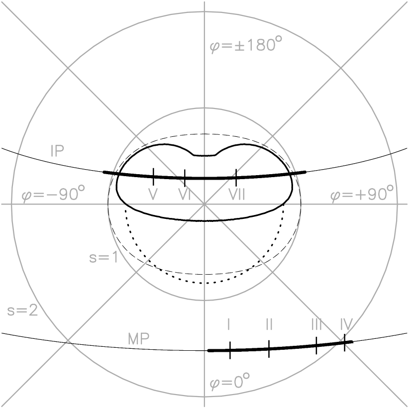
Figure 7: The polar cap map of PSR B1055–52 based on the assumption that both poles have identical structure so that we can “reflect” the observed IP mapping in the horizontal axis. The conventional polar cap size of an aligned rotator is indicated by the circle with radius $s=1$. The dashed ellipse shows the polar cap including meridional compression. The fieldlines inside the kidney-shaped area are open and do not pass through any null line. The top and bottom solid curves are the lines of sight for the MP and IP respectively, where the active portions (assuming an emission height of $0.07R_{\mathrm{LC}}$) are the thicker parts of the curves. The location of the peaks are indicated as well (see Fig. 1). The dotted semi-circle indicates approximately the footprints of the fieldlines on which $\gamma$-rays are thought to be produced.

Having chosen a preferred (maximum) height, we may use the geometric solution of Fig. 6 to generate a map of the polar cap of PSR B1055–52. The result is shown in Fig. 7 and combines the IP and MP on a single pole, thereby assuming that the emission structure at both poles is identical. Obviously, because we only have information about the line of sight which passes over different parts of the polar cap of the MP and IP, we cannot know whether this assumption is true. It must be borne in mind that both the IP and MP are observed on the same meridional planes of $\varphi$ (i.e. they both are viewed below the magnetic axis in Fig. 5), and in Fig. 7 the IP line of sight traverse has been “reflected” in the horizontal axis. This reflection ensures that a point in the polar map is associated with fieldlines which have identical geometric properties for both the MP and IP. The circle $s=1$ corresponds to the footprints of the last closed fieldlines of an aligned dipole touching the light cylinder. For non-aligned dipoles the polar cap shape gets distorted by meridional compression (e.g. Biggs 1990b). The predicted shape for a dipole field inclined at $75^{\circ}$ is shown as the dashed oval in Fig. 7. However, it must be noted that even models which take into account the distortion of the magnetic field lines close to the light cylinder predict roughly circular beams (e.g. Romani & Yadigaroglu 1995).

In Fig. 7 we also indicate the kidney-shaped region within which fieldlines of a dipole inclined at $75^{\circ}$ do not cross the null surface inside the light cylinder. This shape is numerically derived by determining for each dipole fieldline whether the null surface $\mathbf{\Omega}\cdot\mathbf{B}=0$ is penetrated within the light cylinder. It can also be determined analytically (Qiao et al. 2004). In the upper part of the polar map the null surface will lie at a great distance from the polar region (see Fig. 5), but in the lower section it may be close enough to the star to set up an active outergap. We also indicate the approximation of the footprints of the $w=0.18$ fieldlines, argued by Watters et al. (2008) to be the fieldlines on which the $\gamma$-ray emission is produced (dotted semi-circle in Fig. 7).

Note that the locus of active fieldlines on which the IP is generated is symmetric about $\varphi=0$ and barely extends outside $s=1$. Furthermore, the IP fieldlines, apart from their outer edges, are contained within the kidney-shaped locus of the open fieldlines which do not cross a null surface. It was suggested by Goldreich & Julian (1969) that such fieldlines carry the outflowing current from the pulsar.

By contrast, the footprints of the active MP fieldlines lie well outside $s=1$, extending to radii more that double this value. Strangely, they cover only the latter half of a symmetrically-defined full beam. However, as pointed out above, the MP’s fieldlines will thread the null surface close to the star’s surface (at about 160 km) and the emission will occur in a plasma region usually considered to be inactive and corotating, so we can be sure that the MP is not a traditional polar cap profile.

The solution shown is for $r=0.07R_{\mathrm{LC}}$, which is argued to be the maximum allowed emission height (Sect. 5.2). For smaller emission heights both the line of sight of the MP and the IP will move to larger values of $s$ (see Fig. 6) and the active parts of the lines of sight will start leftwards of their current location (more negative values of $\varphi$).

6 Discussion

In our study of PSR B1055–52 we have focused on investigating the geometry of its magnetosphere. Its wide MP and IP, together with a clearly-positioned single gamma-ray peak, place considerable constraints on any potential model. In an earlier attempt to locate the emission regions, Wang et al. (2006) fitted an RVM model to published figures (Lyne & Manchester 1988) for the pulsar’s PA-swing and did not consider the constraints that aberration and retardation might place on the choice of emission heights. We have been able to exploit new data, gathered at Parkes in recent years, to verify the RVM fit and to attempt a self-consistent model.

One of our principal conclusions is that both the MP and IP are emitted at roughly the same height. The optimum fit ($\alpha_{\mathrm{MP}}=75^{\circ}$, $\beta_{\mathrm{MP}}=36.1^{\circ}$) is in line with earlier results.

This PA fit has a number of interesting implications for PSR B1055–52 which are independent of assumptions about the emission heights. Since $\zeta_{\mathrm{MP}}$ (i.e. $\alpha_{\mathrm{MP}}+\beta_{\mathrm{MP}})$, at $111^{\circ}$ is considerably greater than $90^{\circ}$, our line of sight at the MP must see emission on fieldlines at locations which are above the “null” line (Fig. 5), in or beyond territory normally ascribed to an outergap (as was also noted by Hirotani & Shibata 2002). In fact, on elementary geometric grounds, it must be true for every pulsar with a detected IP that at one pole we are viewing above the null line and at the other below it — a point not widely realised before.

However, in the case of PSR B1055–52 (but not necessarily for all pulsars with IP’s), $\zeta_{\mathrm{IP}}>\alpha_{\mathrm{IP}}$ and so our line of sight at the IP must cross the magnetic axis on fieldlines which do not thread the outergap at the opposite pole (Fig. 7). On these grounds alone, we can expect that emission at the MP and IP will reflect the different conditions of these two regions. This can be contrasted with the emission from PSR B1702–19, where at the MP, in one of its two possible solutions, $\alpha_{\mathrm{MP}}=99^{\circ}$ and $\zeta_{\mathrm{MP}}=91.5^{\circ}$ (Weltevrede et al., 2007). Then, at one pole (IP) we must be viewing fieldlines above the null line and at the other (MP) equivalent fieldlines before they cross the null line, with a greater likelihood of coordinated emission.

Although the radio emission at both poles must come from about the same height, the precise height is not easy to determine. To first-order, aberration at a fixed height simply shifts the entire PA curve to later pulse longitudes by an amount proportional to the height. Thus, as long as the emission height is small compared to the light cylinder radius and unchanged across the profile, we have no way of knowing from the shape of the PA curve by how much it has been shifted. The exceptionally wide MP and IP lead us to believe that, whatever the assumed height, it is impossible to confine the footprints of the emitting regions to a polar cap of conventional dimensions (i.e. defined by last closed dipole fieldlines touching the light cylinder). This requirement is particularly acute for the MP, whose trailing components must lie on fieldlines located about twice the conventional polar radius from the pole. Furthermore, since the fiducial point of the MP profile must lie ahead of the steepest gradient of the PA-swing, the observed MP width will never occupy much more than half its notional beam. Choosing a height less than about 500 km would force the polar cap size to escalate rapidly (see Fig. 6) and therefore a balance has to be struck. Here a height 7 per-cent of the light cylinder radius is assumed, so that the IP emission fills its beam and has footprints at around $s=1$ on the opposite side of the pole (assuming identical polar caps at both poles). This choice also has the advantage that the steep edges of the MP (trailing) and IP (leading) correspond to beam edges (see Figs. 6 and 7). We therefore conclude that the emission height is unlikely to be higher or much lower than 700 km, a typical value for pulsars.

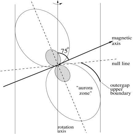
Figure 8: A schematic picture of a physical model for PSR B1055–52, deduced from its radio and $\gamma$-ray profiles. The corotation region, bounded by the fieldline $s=2$, is shaded and lies well within region defined by the last closed fieldline to touch the light cylinder. It is surrounded by an “auroral” zone, which may or may not be entirely closed, but which must support electric fields parallel to its magnetic fieldlines. It makes two different intersections with the null surface, one very close to the star and a second no longer as distant from the surface as in a conventionally-defined corotation region. This may give rise to a complex outergap structure, with pair-created particles continually reflected between the null surfaces. The $\gamma$-ray emission, appropriate to a “middle-aged” pulsar, is located above the outergap, stretching from the null line to the light cylinder.

The kidney shaped central area of Fig. 7, which almost completely encloses the footprints of the IP’s line of sight, highlights a significant consequence of the inferred geometry: the active fieldlines of the IP are open fieldlines which not only do not thread the outergap region beyond the null line close to the surface, but they also do not thread the null surface at any point (assuming a pure dipole geometry as in Fig. 8) before they leave the light cylinder. This suggests that along these fieldlines the pulsar may expel or accrete charged particles without having to encounter any charge sign boundary. Such fieldlines appear to bunch around the magnetic pole bounded by the radial parameter $s=1$, the conventional limit for a polar cap defined by the last closed fieldlines touching the light cylinder. Thus the IP, if observed on a line of sight which missed the MP, would not suggest an unusual geometry.

By contrast, the fieldlines generating the MP have polar footprints well beyond $s=1$ (Fig. 7), although the observed emission region is itself well above the null line (Fig. 5). We are therefore led to the conclusion that in PSR B1055–52’s MP we are seeing emission from regions of the magnetosphere normally regarded as a closed and corotating. A polar cap radius of $s=2$ is the footprint of a fieldline which closes at a distance of only a quarter of the light cylinder radius and which intersects the null line at a height of only 160 km above the polar cap (Fig. 8). In Fig. 7 we see that radio emission occurs on fieldlines with parameters $s=1.5$ (or smaller) to $s=2$, indicating emission on fieldlines for a significant region between the $s=2$ surface shaded in Fig. 8 and the last closed fieldlines ($s\approx{1}$). Radio emission from these fieldlines implies particle acceleration and hence the presence of electric fields parallel to the fieldlines. So it is conceivable that such fieldlines are open and cross the light cylinder (as they do, for example, in the models of aligned magnetospheres with reduced corotation regions given by Goodwin et al. 2004). The closeness of the outergap to the neutron star surface may lead to an active outergap accelerator merging with the polar gap (see Hirotani & Shibata 2002; Hirotani 2006; Muslimov & Harding 2004b; Qiao et al. 2004) and the much reduced corotating region (shaded region in Fig. 8).

Alternatively, the quasi-closed region between fieldlines $s=1$ and $s=2$ can be seen as an auroral zone, analogous to those known to be present in the planets, in which accretion from a debris disk may occur and modulate the radio signal (Cordes & Shannon 2008; Luo & Melrose 2007). In fact, accretion could modulate the entire outergap region through an injection of charge (Hirotani & Shibata 2002). Since all the surface $s=2$ is now so close to the neutron star, it is not impossible to envisage interaction between the two null surfaces which intersect it in the meridional plane (Fig. 8). Possibly “gaps” arise at both at which pair-creation may be stimulated by thermal X-rays from the star’s surface leading to secondary particles “bouncing” between the gaps and stimulating the observed MP emission.

Whatever conditions are present in the envelope between $s=2$ and $s=1$, PSR B1055–52’s $\gamma$-rays are almost certainly generated relatively close to the light cylinder above an outer gap which stretches from the last closed fieldline (whether $s=1$ or $s=2$) towards the light cylinder. Unlike most other $\gamma$-ray pulsars, B1055–52 has a single broad peak which is shown by Watters et al. (2008) to match closely to the geometric predictions of the outergap model of Romani (1996), lying on a fieldline with $s=0.82$. Outergaps with $\gamma$-ray emission regions lying significantly above the last closed fieldline are thought to be a feature of relatively “old” pulsars, as PSR B1055–52 indeed is by the standards of known $\gamma$-ray pulsars. The fact that the $\gamma$-ray pulse overlaps the phase of the MP indicates that both regions point to us at about the same time, which lends support to our model (Fig. 8).

Our conclusions about the geometry of PSR B1055–52 result from a rigid application of the RVM model to high-quality data, taking into account the expected effects from aberration. We are convinced that this pulsar emits radiation from fieldlines lying well outside the conventionally-defined polar cap boundary. Consequently, we would question the common assumption that all pulsars have closed, quiescent, corotating regions stretching to the light cylinder. Possibly this only occurs after the outergap has become inactive, so that energetic (high $\dot{E}$) pulsars can often have wide radio profiles, as observed (Weltevrede & Johnston, 2008). Large polar caps might also help explaining the inconsistency found in calculating emission heights of energetic pulsars using last-closed-fieldline methods (Weltevrede & Johnston, 2008).

An unsatisfactory aspect of our model is the one-sidedness of the MP emission region. This might arise from the very different azimuthal trajectories which particles on the trailing and leading halves must take. On the trailing half they flow counter to the sense of the pulsar’s rotation and can smoothly cross the light cylinder to the wave zone. However, those leaving the leading half of the polar cap will increase speed and hence Lorentz factor as they gain height on corotating fieldlines. It has been suggested that this may lead to additional pair-creation and high-energy emission as the particles free themselves from fieldlines near the light cylinder (Mestel et al. 1976; da Costa & Kahn 1982), but subsequent screening and its consequences for radio emission have not been considered.

Appendix A Trigonometric relations

We are interested to find the relation between the observed pulse longitude and the magnetic coordinates $\rho$ (the angular distance from the magnetic pole) and $\varphi$ (the azimuthal angle around the magnetic pole). This coordinate transformation can be derived using spherical geometry on the celestial sphere of the pulsar. Two trigonometric relations which can be used are the sine and cosine rules for sides (e.g. Smart 1960)

$$\frac{\sin a}{\sin A} = \frac{\sin b}{\sin B}=\frac{\sin c}{\sin C}$$ (7)

$$\cos a = \cos b\cos c+\sin b\sin c\cos A.$$ (8)

See the top panel of Fig. 9 for the definitions of the angles in these equations.

The openings angle of the beam can be derived by applying the cosine rule for sides (Eq. 8) on the triangle plotted in the bottom panel of Fig. 9:

$$\cos\rho=\cos\alpha\cos\zeta+\sin\alpha\sin\zeta\cos\left(\Delta\phi\right)$$ (9)

(Gil et al. 1984). Here $\Delta\phi$ is the pulse longitude measured from the fiducial plane. In the case of a profile which is symmetric around the fiducial plane $\Delta\phi=W/2$.

The azimuthal angle $\varphi$ can be derived by using Eq. 7 on the same triangle plotted in the bottom panel of Fig. 9 and one directly obtains

$$\sin\varphi=\frac{\sin\zeta\sin\Delta\phi}{\sin\rho}$$ (10)

(Gupta et al., 2004). It can be shown that this equation is equivalent to the following expression which is used by Wang et al. (2006):

$$\tan\left(\frac{\pi-\varphi}{2}\right)=\sqrt{\frac{\sin\left(p-\alpha\right)\sin\left(p-\rho\right)}{\sin p\sin\left(p-\zeta\right)}},$$ (11)

where $p=\frac{1}{2}\left(\alpha+\zeta+\rho\right)$.

Figure 9: Top plot: A spherical triangle. The angular lengths of the sides of the triangle are the angles $a$, $b$ and $c$, while $A$, $B$ and $C$ are the angles between the sides of the triangle measured on the surface of the sphere. Bottom plot: A triangle on the celestial sphere used to derive the half openings angle of the beam $\rho$ and the azimuthal angle of a fieldline $\varphi$. The line of sight makes an angle $\zeta$ with the rotation axis and and the magnetic axis makes an angle $\alpha$ with the rotation axis.

References

- Becker & Trümper (1997) Becker W., Trümper J., 1997, A&A, 326, 682
- Biggs (1990a) Biggs J. D., 1990a, MNRAS, 246, 341
- Biggs (1990b) Biggs J. D., 1990b, MNRAS, 245, 514
- Blaskiewicz et al. (1991) Blaskiewicz M., Cordes J. M., Wasserman I., 1991, ApJ, 370, 643
- Cheng et al. (1986) Cheng K. S., Ho C., Ruderman M., 1986, ApJ, 300, 522
- Combi et al. (1997) Combi J. A., Romero G. E., Azcárate I. N., 1997, Ap&SS, 250, 1
- Cordes & Lazio (2002) Cordes J. M., Lazio T. J. W., 2002, astro-ph/0207156
- Cordes & Shannon (2008) Cordes J. M., Shannon R. M., 2008, ApJ, 682, 1152
- da Costa & Kahn (1982) da Costa A. A., Kahn F. D., 1982, MNRAS, 199, 211
- Damour & Taylor (1992) Damour T., Taylor J. H., 1992, Phys. Rev. D, 45, 1840
- Daugherty & Harding (1996) Daugherty J. K., Harding A. K., 1996, ApJ, 458, 278
- Dyks (2008) Dyks J., 2008, MNRAS, 391, 859
- Dyks & Rudak (2003) Dyks J., Rudak B., 2003, ApJ, 598, 1201
- Everett & Weisberg (2001) Everett J. E., Weisberg J. M., 2001, ApJ, 553, 341
- Gangadhara & Gupta (2001) Gangadhara R. T., Gupta Y., 2001, ApJ, 555, 31
- Gil et al. (1984) Gil J. A., Gronkowski P., Rudnicki W., 1984, A&A, 132, 312
- Goldreich & Julian (1969) Goldreich P., Julian W. H., 1969, ApJ, 157, 869
- Goodwin et al. (2004) Goodwin S. P., Mestel J., Mestel L., Wright G. A. E., 2004, MNRAS, 349, 213
- Gupta et al. (2004) Gupta Y., Gil J., Kijak J., Sendyk M., 2004, A&A, 426, 229
- Hibschman & Arons (2001) Hibschman J. A., Arons J., 2001, ApJ, 546, 382
- Hirotani (2006) Hirotani K., 2006, ApJ, 652, 1475
- Hirotani & Shibata (2002) Hirotani K., Shibata S., 2002, ApJ, 564, 369
- Holloway (1973) Holloway N. J., 1973, Nature, 246, 6
- Johnston (2002) Johnston S., 2002, Pub. of the ASA, 19, 277
- Karastergiou & Johnston (2007) Karastergiou A., Johnston S., 2007, MNRAS, 380, 1678
- Kijak & Gil (1997) Kijak J., Gil J., 1997, MNRAS, 288, 631
- Luo & Melrose (2007) Luo Q., Melrose D., 2007, MNRAS, 378, 1481
- Lyne & Manchester (1988) Lyne A. G., Manchester R. N., 1988, MNRAS, 234, 477
- McCulloch et al. (1976) McCulloch P. M., Hamilton P. A., Ables J. G., Komesaroff M. M., 1976, MNRAS, 175, 71P
- McCulloch et al. (1978) McCulloch P. M., Hamilton P. A., Manchester R. N., Ables J. G., 1978, MNRAS, 183, 645
- Manchester & Lyne (1977) Manchester R. N., Lyne A. G., 1977, MNRAS, 181, 761
- Manchester et al. (1975) Manchester R. N., Taylor J. H., Huguenin G. R., 1975, ApJ, 196, 83
- Mestel et al. (1976) Mestel L., Wright G. A. E., Westfold K. C., 1976, MNRAS, 175, 257
- Mitra & Rankin (2002) Mitra D., Rankin J. M., 2002, ApJ, 577, 322
- Muslimov & Harding (2004a) Muslimov A. G., Harding A. K., 2004a, ApJ, 606, 1143
- Muslimov & Harding (2004b) Muslimov A. G., Harding A. K., 2004b, ApJ, 606, 1143
- Noutsos et al. (2008) Noutsos A., Johnston S., Kramer M., Karastergiou A., 2008, MNRAS, 386, 1881
- Ögelman & Finley (1993) Ögelman H., Finley J. P., 1993, ApJ, 413, L31
- Qiao et al. (2004) Qiao G. J., Lee K. J., Wang H. G., Xu R. X., Han J. L., 2004, ApJ, 606, L49
- Radhakrishnan & Cooke (1969) Radhakrishnan V., Cooke D. J., 1969, Astrophys. Lett., 3, 225
- Rankin (1983) Rankin J. M., 1983, ApJ, 274, 333
- Romani (1996) Romani R. W., 1996, ApJ, 470, 469
- Romani & Yadigaroglu (1995) Romani R. W., Yadigaroglu I.-A., 1995, ApJ, 438, 314
- Smart (1960) Smart W. M., 1960, Text-Book on Spherical Astronomy, 6th ed.. Cambridge University Press, Cambridge, England
- Smith et al. (2008) Smith D. A., Guillemot L., Camilo F., Cognard I., Dumora D., Espinoza C., Freire P. C. C., Gotthelf E. V., Harding A. K., Hobbs G. B., Johnston S., Kaspi V. M., Kramer M., Livingstone M. A., Lyne A. G., Manchester R. N., Marshall F. E., et al. 2008, A&A, 492, 923
- Taylor et al. (1993) Taylor J. H., Manchester R. N., Lyne A. G., 1993, ApJS, 88, 529
- Thompson et al. (1999) Thompson D. J., Bailes M., Bertsch D. L., Cordes J., D’Amico N., Esposito J. A., Finley J., Hartman R. C., Hermsen W., Kanbach G., Kaspi V. M., Kniffen D. A., Kuiper L., Lin Y. C., Manchester R., Matz S. M., Mayer-Hasselwander H. A., Michelson P. F., et al. 1999, ApJ, 516, 297
- Vaughan & Large (1972) Vaughan A. E., Large M. I., 1972, MNRAS, 156, 27P
- Wang et al. (2006) Wang H. G., Qiao G. J., Xu R. X., Liu Y., 2006, MNRAS, 366, 945
- Watters et al. (2008) Watters K., Romani R. W., Weltevrede P., Johnston S., 2008, ApJ in press (astro-ph/0812.3931)
- Weltevrede & Johnston (2008) Weltevrede P., Johnston S., 2008, MNRAS, 391, 1210
- Weltevrede et al. (2007) Weltevrede P., Wright G. A. E., Stappers B. W., 2007, A&A, 467, 1163