Gravitational Space Dilation

Abstract

We point out that, if one accepts the view that the standard second on an atomic clock is dilated at low gravitational potential (ordinary gravitational time dilation), then the standard meter must also be dilated at low gravitational potential and by the same factor (gravitational space dilation). These effects may be viewed as distortions of the time and length standards by the gravitational field, and measurements made with these distorted standards can be “corrected” by means of a conformal transformation applied to the usual spacetime metric of general relativity. Because the amount of gravitational time dilation depends on the location of the observer, the “correction” of the metric is specific to a particular observer, and we arrive at a “single-observer” picture (or SO-picture) of events in a static gravitational field. The surprising feature of this single-observer picture is a substantial simplification of interpretation and formalism for numerous phenomena in a static gravitational field as compared to the conventional “many-observer” interpretation (or MO-picture) of general relativity. The principle results of the single-observer picture include: (1) the speed of light has the invariant value $c$ everywhere (as it does in the MO-picture), (2) light rays propagate on geodesics of the single-observer three-space, (3) the relativistic radar echo delay, when a massive body is brought near the radar propagation path, is attributed to an increase in the three-space distance between transmitter and target, (4) the gravitational bending of light and the precession of perihelion are due solely to the curvature of the single-observer’s three-space, (5) particle motion in a static gravitational field is closely analogous to that in Newtonian mechanics permitting a clear comparison of classical and relativistic motions without approximation, (6) the exact field equation for the “gravitational potential” in the single-observer picture is the linear Poisson equation of Newtonian gravitation theory, (7) the three-space Maxwell equations in the single-observer picture have the same vector forms as in flat space (not so in the many-observer picture), (8) as a consequence of (7), many standard electrodynamic results, such as Ampere’s law and Faraday’s law are valid in the single-observer three-space, (9) a solar-system test of gravitational space dilation is suggested that seems to be within the capability of existing technology, and finally (10) thermal equilibrium in a gravitational field is characterized by uniform temperature in the SO-picture (not so in the standard MO-picture).

I INTRODUCTION

We motivate the viewpoint taken in this paper with the following “Parable of the self-centered observer.”

A “self-centered” observer at $O$ in a static gravitational field

$$d\bar{s}^{2}=\bar{g}_{00}c^{2}d\bar{t}^{2}+\bar{g}_{ij}dx^{i}dx^{j},$$ (1)

observes a standard clock at rest at point $P$ ticking slower than his own standard clock of identical construction (gravitational time dilation). Being intolerant of other viewpoints, observer $O$ concludes that the observer at $P$ uses a faulty time standard and that a correction of $P$’s time measurement is required.

Observer $O$ also concludes that the length standard used by observer $P$ is in error because the standard meter is defined as the distance light travels in time $\tau_{m}=(1/299,792,458)\ s$ at the defined speed $c$ of exactly $299,792,458\ m/s$, and so an error in time measurement by $P$ translates into an error in his length standard (the length standard at $P$ is “too long”, in the view of observer $O$, because $P$’s slow clock allows light to travel too long a time in defining his standard).

A moments thought by observer $O$ convinces him that, if [as implied by (1)],

$$\mathcal{R}=\left[\frac{\bar{g}_{00}(P)}{\bar{g}_{00}(O)}\right]^{1/2}$$ (2)

is the rate of $P$’s clock as measured with $O$’s time standard, then the “incorrect” time and length intervals ($d\bar{\tau}$ and $d\bar{\ell}$) measured by $P$ using “faulty” local standards are related to the “true” length and time intervals ($d\tau$ and $d\ell$) at $P$ by equations

$$d\tau = \frac{d\bar{\tau}}{\mathcal{R}}$$ (3a)

$$d\ell = \frac{d\bar{\ell}}{\mathcal{R}}.$$ (3b)

Equation (3a) expresses the well-tested gravitational time-dilation effect. Observer $O$ concludes that both time and length are dilated at $P$, and by the same factor. He finds this result satisfying in a relativistic theory where space and time are “made of the same stuff” and therefore ought to be affected similarly by a gravitational field. From this point on, he speaks not of time dilation alone but of space dilation as well, or of “spacetime dilation”.

The scale change described by equations (3) is represented in spacetime notation by the conformal transformation $ds^{2}=d\bar{s}^{2}/\mathcal{R}^{2}$ of metric (1). Under this transformation the proper time $d\bar{\tau}$ [$=(-d\bar{s}^{2}/c^{2})^{1/2}$] of observer $P$ goes over into the proper time $d\tau$ [$=(-ds^{2}/c^{2})^{1/2}$] of observer $O$ as in Eq. (3a), and the proper distance $d\bar{\ell}$ ($d\bar{\ell}^{2}=\bar{g}_{ij}dx^{i}dx^{j}$) of observer $P$ goes over into the proper distance $d\ell$ of observer $O$ in accordance with Eq. (3b). Therefore the “correct” metric in the view of our self-centered observer (“corrected” for gravitational time dilation) reads

$$ds^{2} = d\bar{s}^{2}/\mathcal{R}^{2}$$ (4)

$$= \frac{\bar{g}_{00}(P)c^{2}d\bar{t}^{2}}{[\bar{g}_{00}(P)/\bar{g}_{00}(O)]}+\frac{\bar{g}_{ij}dx^{i}dx^{j}}{\mathcal{R}^{2}}$$

$$= -c^{2}dt^{2}+g_{ij}dx^{i}dx^{j},$$

where we have trivially rescaled the coordinate time by a constant factor depending on $O$’s location ($t=[-\bar{g}_{00}(O)]^{1/2}\bar{t}$), and have identified

$$g_{ij}=\bar{g}_{ij}/\mathcal{R}^{2}$$ (5)

as the spatial metric tensor observer $O$ would regard as correct ($d\ell^{2}=g_{ij}dx^{i}dx^{j}$ is the appropriate spatial metric in observer $O$’s opinion).

The usual spacetime picture in general relativity (the one based on metric $d\bar{s}^{2}$) is operationally founded on the notion of a large number of observers distributed over space; each making local measurements with locally defined standards of time and length (the “ten thousand local witnesses” in the words of Taylor and Wheeler) Taylor . We shall refer to this as the “many-observer picture” (MO-picture) and the associated metric $d\bar{s}^{2}$ as the metric of many-observer spacetime (or MO-spacetime for short), and we shall call the spatial section with metric $d\bar{\ell}^{2}=\bar{g}_{ij}dx^{i}dx^{j}$ many-observer space (or MO-space). Similarly we shall refer to the picture based on the metric $ds^{2}$ as the single-observer picture (or single-observer spacetime, or SO-spacetime), and we shall call the spatial section with metric $d\ell^{2}=g_{ij}dx^{i}dx^{j}$ Gaussian space (or SO-space or G-space). The reason for calling the single-observer space “Gaussian space” will become apparent in Sec. II [We are using the over-bar to denote the standard MO-picture variables and no over-bar for SO-picture variables because most of the equations to follow are in the SO-picture and the notation is thereby simplified. We use the same (unbarred) spatial coordinates $x^{i}$ in both pictures.].

One purpose of the present paper is to show that gravitational space dilation, like gravitational time dilation, is measurable (at least in principle) and that the relativistic radar echo delay experiment may be interpreted as a test of gravitational space dilation. A second purpose of this paper is to show that the single-observer picture is convenient for the calculation and interpretation of various results in general relativity. But before doing so, we address an objection that may already be in the mind of the reader.

Generally speaking, measurement from a distance is problematic in general relativity. Therefore we should like to emphasize that the single-observer picture does not involve actual measurement from a distance. In a static gravitational field, regular light pulses from a stationary beacon cross any stationary point at the same rate they are emitted (in coordinate time) because each pulse traverses an identical time-independent field. Therefore slave clocks distributed at rest over space and ticking each time they receive a beacon pulse from $O$ all tick at the same rate (no gravitational slowing), and any one of them can be used to reproduce $O$’s time and length standards at its location. Observer $O$’s time unit transferred to $P$ is the time between ticks on the slave clock at $P$, and observer $O$’s length standard transferred to $P$ is the distance light travels at $P$ in time $\tau_{m}$ (=1/299,792,458 seconds) as read on the slave clock at $P$. The metric $ds^{2}$ describes the results of measurements made locally with the slave-clock standards, whereas the metric $d\bar{s}^{2}$ describes the results of measurements made with time and length standards based on local freely-running, gravitationally-slowed clocks. Strictly speaking, this is what we mean when we say that $O$ applies his own time and length standards at $P$. It is the same logic used in comparing clock rates in the gravitational time-dilation experiment. Therefore, no actual measurement from a distance is involved, though, for convenience, we shall often speak loosely in such terms.

Incidentally, the slave clock readings determine a time at each point of space. If the slave clocks are synchronized by the Einstein synchronization procedure, then they read the coordinate time $t$ ($=[-\bar{g}_{00}(O)]^{1/2}\bar{t}$) introduced above for the metric $ds^{2}$. This is an operational definition of the time $t$.

The metrics $d\bar{s}^{2}$ and $ds^{2}$ are physically equivalent and conformally equivalent. They represent the same spacetime geometry measured with different standards of length and time Remark . Nevertheless, we shall refer to the different picture as “different spacetimes” because “invariants” such as the curvature scalars $\bar{R}$ and $R$ have different values in the two pictures and the metrics $d\bar{s}^{2}$ and $ds^{2}$ are not related by a coordinate transformation.

One important result which is the same in both the single-observer and many-observer pictures concerns the local speed of light. In MO-spacetime the local speed of light is everywhere $c$: $d\bar{\ell}/d\bar{\tau}_{0}=c$ or $d\bar{s}=0$ (here $d\bar{\tau}_{0}$ is the proper time on a local freely-running rest clock). Under the transformation (3a)-(3b) [or (4)] the local light speed retains this value: $d\ell/d\tau_{0}=(d\bar{\ell}/\mathcal{R})/(d\bar{\tau}_{0}/\mathcal{R})=d\bar{\ell}/d\bar{\tau}_{0}=c$ (or $ds=0$), where now $d\tau_{o}=dt$ is local slave-clock time, or “observer $O$’s time” when we speak loosely. Hence we have

Result I: In the single-observer picture the speed of light $d\ell/dt$ has the invariant value $c$ everywhere and at all times.

The same argument shows that any speed has the same value in MO-space and in SO-space (or Gaussian space), i.e., $v=\bar{v}$.. Note that, according to metric (4), the single-observer rest-clock proper time $\tau_{0}$ is the same as the coordinate time $t$, and we use the two interchangeably.

In Sec. II we show that light rays follow geodesics of the single-observer three space (geodesics of Gaussian space) and discuss some simple consequences of this result. Sec. III addresses the radar propagation problem, and concludes that radar from $O$ directly measures the single-observer distance $\int d\ell$, and the relativistic radar echo delay experiment Shapiro may be interpreted as an increase in this distance as the solar mass comes near the radar propagation path. Sec. IV treats particle motion in a static gravitational field. Here we find a close analogy between particle motion in Gaussian space and that in Newtonian gravitational mechanics. This permits a clear comparison of classical and relativistic motions without introducing approximations, e.g., perihelion precession is attributed solely to the curvature of Gaussian space in the SO-picture. In Sec. V, we find that the gravitational acceleration of a particle at rest in Gaussian space, $\mathbf{g}_{0}=-\nabla\Phi$, is determined by the linear Poisson equation $\nabla^{2}\Phi=-4\pi G\rho_{g}$ of Newtonian gravitation theory (here seen to be an exact relativistic result)—the only difference between the Newtonian and relativistic gravitation theories being the non-Euclidean geometry of the Gaussian three-space and an energy dependent factor $(\bar{m}c^{2}/E)^{2}$ in the gravitational acceleration $\mathbf{g}=-(\bar{m}c^{2}/E)^{2}\nabla\Phi$ when the particle velocity is nonzero. In Sec. VI, the three-space Maxwell equations are derived for Gaussian space and are found to have the same vector forms as in flat space (not so in the MO-picture). This leads to a number of electromagnetic theorems, e.g., Amperes law and Faraday’s law, that hold in Gaussian space but do not hold in the usual MO-picture. In Sec. VII we suggest a solar-system test of gravitational space dilation involving radar measurements. Sec. VIII presents a number of applications of the space-dilation formalism chosen to illustrate how very different the physical interpretations of phenomena can be in the MO- and SO-pictures. The paper concludes in Sec. IX with a summary of results.

II LIGHT RAYS AS SPATIAL GEODESICS

Fermat’s principle in MO-space Misner states that, in a static gravitational field, the path taken by light between points $P_{1}$ and $P_{2}$ is the one that minimizes the coordinate time elapsed in propagating between the two points,

$$\delta\int_{P_{1}}^{P_{2}}d\bar{t}=0.$$ (6)

Using the null condition $d\bar{s}^{2}=0$ and (2) in Eq. (1), we find that (6) can be written as

$$\delta\int_{P_{1}}^{P_{2}}\left[\frac{\bar{g}_{ij}}{\mathcal{R}^{2}}\frac{dx^{i}}{dq}\frac{dx^{j}}{dq}\right]^{1/2}dq=0$$ (7)

for any parameterization $x^{i}(q)$ of the path between $P_{1}$ and $P_{2}$. But Eq. (7) is precisely the condition for the single-observer path length between the two points to be minimum,

$$\delta\int_{P_{1}}^{P_{2}}d\ell=0,$$ (8)

where $d\ell^{2}=g_{ij}dx^{i}dx^{j}$ is the spatial part of the single-observer metric (4).

Result II: Light rays in a static gravitational field are geodesics of the single-observer spatial metric $d\ell^{2}=g_{ij}dx^{i}dx^{j}$, i.e., geodesics of Gaussian space.

This result can be understood by noting that, in a space where the light speed $d\ell/dt=c$ is everywhere the same and the differential $dt$ is exact (so that the speed $d\ell/dt$ is integrable), a principle of least time is equivalent to a principle of least distance. This does not hold true in MO-space where, although each local observer measures the same light speed $d\bar{\ell}/d\bar{\tau}_{0}=c$, the clocks of different observers run at different rates (the local proper time differential $d\bar{\tau}_{0}$ is not exact) and it cannot be concluded that the MO-space distance is least. Indeed, it is well known that light rays do not travel the geodesics of the spatial metric $d\bar{\ell}^{2}=\bar{g}_{ij}dx^{i}dx^{j}$ of MO-space.

Let us apply Result II to the Schwarzschild line element

$$d\bar{s}^{2}=-(1-2m/r)c^{2}d\bar{t}^{2}+\frac{dr^{2}}{(1-2m/r)}+r^{2}d\Omega^{2}.$$ (9)

where $d\Omega^{2}=d\theta^{2}+sin^{2}\theta d\phi^{2}$. The rate of a clock at rest at $P$ (coordinates $r,\theta,\phi$) as viewed by an observer $O$ at $r_{0}=\infty$ [Eq. (2)] is

$$\mathcal{R}=\left(1-\frac{2m}{r}\right)^{1/2}.$$ (10)

Hence the spatial part of the single-observer metric (4), specialized to the $\theta=\pi/2$ plane, reads

$$d\ell^{2}=\frac{1}{(1-2m/r)}\left[\frac{dr^{2}}{(1-2m/r)}+r^{2}d\phi^{2}\right].$$ (11)

Using $\phi$ as the parameter for the trajectory $r(\phi)=1/u(\phi)$, we easily obtain the two-space geodesic equation in this Gaussian space:

$$\frac{d^{2}u}{d\phi^{2}}+u=3mu^{2}.$$ (12)

This is the familiar trajectory equation for light in the gravitational field of the sun (in which case $m=1.48\ km$), here obtained as a spatial geodesic of G-space. The complete description of light propagation for the single observer consists of the trajectory $r(\phi)$ together with Result I stating that light travels this trajectory with speed $d\ell/dt=c$. (Here the single-observer time $t$ is just the coordinate time $\bar{t}$ because the observer is at infinity.).

The interpretation of light deflection is simple in Gaussian space. According to Result II, light is bent by a static gravitational field solely because it is traveling the shortest path in the non-Euclidean G-space with metric

$$d\ell^{2}=\frac{1}{(1-2m/r)}\left[\frac{dr^{2}}{(1-2m/r)}+r^{2}d\Omega^{2}\right],$$ (13)

where $d\Omega^{2}=d\theta^{2}+sin^{2}\theta d\phi^{2}$ (Here we are not restricted to the $\theta=\pi/2$ plane.)

MO-Picture Interpretation: The interpretation of light deflection in MO-spacetime is more complicated. In several books on general relativity we find diagrams suggesting that gravitational light deflection may be attributed to the non-Euclidean nature of three-space, but we are often not warned that “the light ray is not a geodesic line in three-dimensional space” (the quote is from Pauli Pauli ). In Will Will1 we correctly learn that half of the light deflection may be attributed to the non-Euclidean MO-space and half to the principle of equivalence applied in a sequence of freely falling reference frames along the ray, as first employed by Einstein Einstein1 .

We now see that light rays as spatial geodesics is a valid concept provided we adopt the “self-centered” view of the single observer who uses his own length standard for distance measurement throughout space in place of the locally defined standards.

A rewording of Result II states that the three-velocity $c^{k}=dx^{k}/dt$ of a photon (the tangent vector to the light ray) undergoes parallel transport in G-space. This follows from Result II by taking $q=t$ as the affine parameter for the ray $x^{k}(t)$. The three-space geodesic equation [$d^{2}x^{k}/dt^{2}+\Gamma^{k}_{ij}(dx^{i}/dt)(dx^{j}/dt)=0$] is then the equation of parallel transport [$dc^{k}/dt=-\Gamma^{k}_{ij}c^{i}dx^{j}/dt$] for the photon three-velocity $c^{k}$ in G-space, and the parallel transport of $c^{k}$ leaves the magnitude of this three-vector invariant at value $c$ (Result I).

Because the geodesics of G-space are the paths of light rays, the non-Euclidean features of this space are measurable optically. Fig. 1 shows three intersecting light rays, each bent by the sun’s gravitational field.

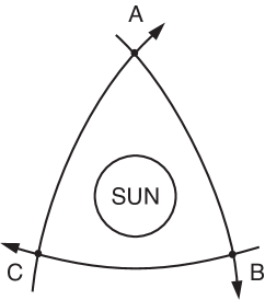
Figure 1: Three gravitationally bent light rays form a triangle $ABC$ about the sun. The sum of the interior angles is greater than two right angles. This shows directly that the single-observer three-space (G-space) is non-Euclidean, because the light rays are geodesics of G-space.

The interior angles of the triangle formed by these rays sum to greater than $\pi$ radians; an earmark of non-Euclidean geometry. Therefore, the measured deflection of light by the sun’s gravitational field is direct evidence for the curvature of G-space (It is not direct evidence for a non-Euclidean MO-space, because light rays are not geodesics of MO-space).

In Euclidean geometry, a “biangle” is a rather uninteresting closed figure with two equal sides, two equal angles ($\alpha=\beta=0$), and zero area (two overlapping line segments). However, in non-Euclidean geometry, the biangle can open into a non-trivial figure with finite area and finite vertex angles. The “football shaped” figure formed by two lines of longitude on a sphere meeting at the poles is an example of a non-trivial biangle; an “equilateral biangle”.

Two light rays diverging from a point and brought back together by the gravitational attraction of a mass $M$, as in Fig. 2, form a biangle in the G-space of observer $O$.

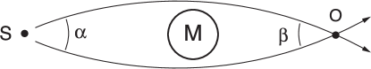
Figure 2: Two light rays diverging from source $S$ are bent by the gravitational field of mass $M$ and intersect at observer $O$. The closed two-sided figure with vertex angles $\alpha$ and $\beta$ is a non-trivial “biangle” in the G-space of observer $O$. The existence of a non-trivial biangle (geodesics initially diverging from a point and then coming together) implies that this G-space is non-Euclidean. It follows that the double images of a quasar produced by gravitational lensing offer direct evidence for a non-Euclidean G-space.

The existence of a biangle with non-zero vertex angles implies that the G-space around mass $M$ is non-Euclidean. We may conclude that the double (or multiple) images of quasars, formed by gravitational lensing also provide direct evidence for a non-Euclidean G-space geometry.

Probably the first attempt to detect non-Euclidean features of three-dimensional space was that of Carl Friedrich Gauss. It is reported that Gauss used light beams between mountain tops in an attempt to detect a deviation from the Euclidean theorem stating that the sum of the interior angles of a triangle equals two right angles Bonola . In this experiment Gauss found it natural to assume that light propagates along geodesics of the three-space. Because the geodesic character of light rays is the central feature of the single-observer three space, it seems natural to refer to this space as “Gaussian space” (or “G-space” for short) as we have been doing already for a while now.

We note in passing that, when a carpenter looks along the edge of a piece of lumber to see if it is “straight,” he is using the Gaussian-space definition of “straight,” namely the path of a light ray as the straightest possible curve in three-dimensional space.

III RADAR ECHO DELAY

Consider the G-space distance $\ell$ measured along a light ray from the observer at $O$ to the point $P$. Because the single observer at $O$ sees the same light speed $d\ell/dt=c$ everywhere (and because the differential $dt$ is exact, i.e., the derivative $d\ell/dt$ is integrable), it follows that the distance $\ell$ is traversed in time $\Delta t=\ell/c$. If light travels from $O$ to $P$ and back to $O$, the total elapsed time on the clock at $O$ is given by $\Delta t=2\ell/c$, or $\ell=c\Delta t/2$, namely the radar range formula. We thus arrive at

Result III: The G-space distance measured along a light ray from observer $O$ to point $P$ (the geodesic distance determined by the spatial metric $d\ell^{2}=g_{ij}dx^{i}dx^{j}$) is the radar distance from $O$ to $P$ measured using a radar unit at $O$.

This is a useful observation. It tells us that, in a static gravitational field, when a single observer chooses length and time standards throughout space consistent (in his view) with his own local standards, his natural measure of distance is radar distance. This singles out radar distance as more natural for the single observer than the other possible distance measures (MO-space proper distance, luminosity distance, angular diameter distance, etc.). By the same token, radar is the natural tool for measuring the G-space geometry, since it measures G-space distance directly, at least along light rays from $O$ (actually the G-space metric for observer $O$ is measured by radar from any point and in any direction so long as the radar at that point uses the local slave-clock time $t$ to measure the radar echo delay).

The relativistic radar echo delay has a simple interpretation in G-space. Consider the Schwarzschild geometry in isotropic coordinates:

$$d\bar{s}^{2} = -\left(\frac{1-m/2\rho}{1+m/2\rho}\right)^{2}c^{2}d\bar{t}^{2}$$ (14)

$$+\left(1+m/2\rho\right)^{4}\left(dx^{2}+dy^{2}+dz^{2}\right).$$

Here $x,y,z$ are rectangular coordinate markers and $\rho=\left(x^{2}+y^{2}+z^{2}\right)^{1/2}$.

To an observer at infinity ($\rho_{0}=\infty$), a stationary clock at radial coordinate $\rho$ runs at the rate

$$\mathcal{R}=\frac{\left(1-m/2\rho\right)}{\left(1+m/2\rho\right)}.$$ (15)

Hence the G-space geometry is described by the metric

$$d\ell^{2}=\frac{d\bar{\ell}^{2}}{\mathcal{R}^{2}}=\frac{(1+m/2\rho)^{6}}{(1-m/2\rho)^{2}}\left(dx^{2}+dy^{2}+dz^{2}\right).$$ (16)

Consider the geodesic distance in G-space from Earth (point $E$) to Mars (point $M$) when Mars is near superior conjunction and the radar path $EM$ passes near the sun, as in Fig. 3.

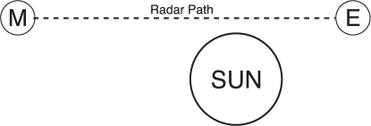
Figure 3: Radar propagates from Earth (E) to Mars (M) and back. The radar path length in Gaussian space is longer when the sun is near the propagation path (superior conjunction) than when the sun is far removed from the propagation path. This accounts for the relativistic radar echo delay.

In the absence of the sun ($m=0$), or when the sun is far from the radar propagation path, the G-space metric (16) is Euclidean ($d\ell^{2}_{0}=dx^{2}+dy^{2}+dz^{2}$), and the geodesic path from $E$ to $M$ is a straight line of some length $\ell_{0}$. With the sun in place near the propagation path ($m=GM_{\odot}/c^{2}$), the G-space metric is given by (16), and the geodesic distance from $E$ to $M$ is increased to $\ell=\int_{E}^{M}d\ell$. Because the speed of light is everywhere $c$ for the single observer, the increase in path length from $E$ to $M$ causes an additional radar delay $\delta t=2(\ell-\ell_{0})/c$ over and above what would be expected in Euclidean space. This is the excess delay measured in the Shapiro relativistic radar echo experiment Shapiro .

Result IV: In the single-observer picture, the relativistic radar echo delay is attributed to an increase in distance between the transmitter and target when a large mass (e.g.,the sun) is brought near the radar propagation path.

Both the bending of light and the excess radar echo delay are nicely pictured by embedding the $\theta=\pi/2$ plane of G-space in Euclidean three-space. The embedding diagram is sketched in Fig. 4.

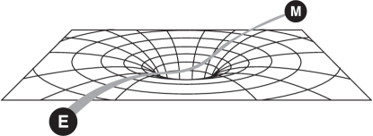
Figure 4: Embedding diagram for the $\theta=\pi/2$ plane of G-space in the neighborhood of the sun (schematic and not to scale). A light ray passing near the sun is deflected because it travels a geodesic path on the embedding surface. A radar pulse is delayed because the sun increases the geodesic distance from Earth $E$ to Mars $M$ when it is near the radar propagation path. The increased distance is attributed to the depression of the embedding surface near the sun.

The curvature of the surface causes deflection of a light ray (a G-space geodesic) and the increased distance from $E$ to $M$ is due to the depression of the surface near the mass $M_{\odot}$.

MO-Picture Interpretation Interpretation of the radar delay is more complicated in MO-spacetime. In MO-space, half of the delay is attributed to an increased path length and half to gravitational time dilation along the propagation path Will2 .

IV PARTICLE MOTION IN G-SPACE

It is of interest to learn how material particles move in the three-space for which light rays define geodesics. We find that the single-observer picture of particle motion is very much closer in spirit to Newtonian mechanics than to the usual formulation in general relativity. This allows a clear comparison of Newtonian and relativistic motions without approximation.

IV.1 Equations of motion

Particles travel on geodesics of MO-spacetime:

$$\delta\int d\bar{\tau}=0,$$ (17)

where $\bar{\tau}$ is the proper time at the moving particle as measured with a locally defined time standard (MO-picture). Using equation (3a), $d\bar{\tau}=\mathcal{R}d\tau$, and noting that the proper time in the SO-picture ($d\tau^{2}=-ds^{2}/c^{2}$) obeys the same motional time dilation formula as in special relativity,

$$d\tau=\sqrt{1-v^{2}/c^{2}}dt,$$ (18)

where $v^{2}=d\ell^{2}/dt^{2}=g_{ij}(dx^{i}/dt)(dx^{j}/dt))$ is the squared speed of the particle in G-space, equation (17) indicates that particle motion is derivable from the three-space Lagrangian

$$L = -\bar{m}c^{2}\mathcal{R}\left(1-\frac{v^{2}}{c^{2}}\right)^{1/2}$$ (19)

$$= -\bar{m}c^{2}\mathcal{R}\left(1-\frac{g_{ij}}{c^{2}}\frac{dx^{i}}{dt}\frac{dx^{j}}{dt}\right)^{1/2},$$

here written in terms of G-space variables. We have added the inessential constant factor $-\bar{m}c^{2}$ for later convenience of interpretation, where $\bar{m}$ is the rest mass in the MO-picture (a constant). From this Lagrangian we obtain the momentum

$$p_{k} = \frac{\partial L}{\partial(dx^{k}/dt)}$$ (20)

$$= \frac{\bar{m}\mathcal{R}v_{k}}{\sqrt{1-v^{2}/c^{2}}}$$

conjugate to coordinate $x^{k}$, where $v_{k}=g_{ki}v^{i}=g_{ki}dx^{i}/dt$. The Hamiltonian

$$H = p_{k}v^{k}-L$$ (21)

$$= \frac{\bar{m}c^{2}\mathcal{R}}{\sqrt{1-v^{2}/c^{2}}}$$

$$= E,$$

is the conserved energy E of the particle. Note that in Gaussian space indices are lowered and raised with $g_{ij}$ and it’s inverse $g^{ij}$, respectively. From the Lagrangian (19) there follows the equation of motion in G-space

$$\frac{d^{2}x^{k}}{dt^{2}}+\Gamma^{k}_{\ ij}\frac{dx^{i}}{dt}\frac{dx^{j}}{dt}=-\left(\frac{\bar{m}c^{2}}{E}\right)^{2}\frac{\partial\Phi}{\partial x_{k}},$$ (22)

where $\Gamma^{k}_{\ ij}=(1/2)g^{kl}(\partial_{j}g_{li}+\partial_{i}g_{lj}-\partial_{l}g_{ij})$ are the G-space Christoffel symbols, we have used the constancy of $E$ in the derivation, and

$$\Phi=\frac{1}{2}c^{2}\mathcal{R}^{2}$$ (23)

is the “Newtonian gravitational potential” in G-space (the justification for this terminology will become apparent in Sec. V). From Eq. (22) we see that, as the particle approaches light speed ($E>>\bar{m}c^{2}$), the term on the right vanishes and the particle moves on a geodesic of G-space, as do photons.

Notice that the Lagrangian

$$L=-mc^{2}\sqrt{1-v^{2}/c^{2}},$$ (24)

the energy

$$E=\frac{mc^{2}}{\sqrt{1-v^{2}/c^{2}}}=\sqrt{c^{2}p^{2}+m^{2}c^{4}},$$ (25)

and the momentum

$$\mathbf{p}=\frac{m\mathbf{v}}{\sqrt{1-v^{2}/c^{2}}}$$ (26)

in G-space all have the same forms as in special relativity, provided we identify the position-dependent quantity

$$m(\mathbf{x})=\bar{m}\mathcal{R}(\mathbf{x})$$ (27)

as the rest mass of the particle in the SO-picture. On this interpretation, the position-dependent rest energy of the particle, $mc^{2}=\bar{m}c^{2}\mathcal{R}$, plays the role of a gravitational potential energy in G-space, as can be seen in the non-relativistic ($v^{2}\ll c^{2}$) limits of the lagrangian (24) [$L=mv^{2}/2-m(\mathbf{x})c^{2}$] and the energy (25) [$E=mv^{2}/2+m(\mathbf{x})c^{2}$].

In fact, the interpretation of the rest energy $m(\mathbf{x})c^{2}$ as a gravitational potential energy is fully relativistic. The G-space energy $E$ and three-momentum $p^{i}$ combine to form a four-vector momentum

$$P^{\mu}=(\frac{E}{c},p^{i})=m\frac{dx^{\mu}}{d\tau},$$ (28)

in the SO-picture. This is related to the MO-picture momentum $\bar{P}^{\mu}\equiv\bar{m}dx^{\mu}/d\bar{\tau}$ by the conformal transformation law

$$P^{\mu}=\mathcal{R}^{2}\bar{P}^{\mu}.$$ (29)

In the absence of non-gravitational forces, the four-momentum $\bar{P}^{\mu}$ is parallel transported in MO-spacetime [$d\bar{P}^{\mu}/d\bar{\tau}+\bar{\Gamma}^{\mu}_{\ \alpha\beta}\bar{P}^{\alpha}dx^{\beta}/d\bar{\tau}=0$]. But this equation is not conformally invariant. In the SO-picture, the four-momentum (28) obeys the equation of motion

$$\frac{DP^{\mu}}{d\tau}\equiv\frac{dP^{\mu}}{d\tau}+\Gamma^{\mu}_{\ \alpha\beta}P^{\alpha}\frac{dx^{\beta}}{d\tau}=-\frac{\partial(mc^{2})}{\partial x_{\mu}}$$ (30)

in which the rest energy $m(\mathbf{x})c^{2}$ manifestly plays the role of a scalar potential energy.

Result V: Although there is no true gravitational force in the MO-picture, i.e., the momentum $\bar{P}^{\mu}$ obeys the “law of inertia” $D\bar{P}^{\mu}/d\bar{\tau}=0$ and is constant in a local inertial frame, the momentum $P^{\mu}=\mathcal{R}^{2}\bar{P}^{\mu}$ of the SO-picture changes due to the action of a gravitational four-force $f^{\mu}=-\partial V/\partial x_{\mu}$ derivable from a scalar potential $V=m(\mathbf{x})c^{2}$ that is the rest energy of the particle in this picture:

$$\frac{DP^{\mu}}{d\tau}\equiv\frac{dP^{\mu}}{d\tau}+\Gamma^{\mu}_{\ \alpha\beta}P^{\alpha}\frac{dx^{\beta}}{d\tau}=-\frac{\partial V}{\partial x_{\mu}}.$$ (31)

Notice that the “Newtonian gravitational potential” $\Phi$, the “gravitational potential energy” $V$, and the “atomic rest-clock rate” $\mathcal{R}$ all contain the same information:

$$\frac{2\Phi}{c^{2}}=\left(\frac{V}{\bar{m}c^{2}}\right)=\mathcal{R}^{2}.$$ (32)

The potential energy $V(\mathbf{x})$ determines the rate of change of momentum $P^{\mu}$, the gravitational potential $\Phi$ (together with the particle mass $\bar{m}$ and its energy $E$) determine the three-acceleration of the particle in G-space [Eq. (22)], and the scale factor $\mathcal{R}(\mathbf{x})$ is the ticking rate of a free-running atomic clock on the time scale of observer O’s local clock.

IV.2 Newtonian Analogy

The exact relativistic equation of motion in G-space (22) is quite similar to the Newtonian equation of motion in curvilinear coordinates

$$\frac{d^{2}x^{k}}{dt^{2}}+\Gamma^{k}_{ij}\frac{dx^{i}}{dt}\frac{dx^{j}}{dt}=-\frac{\partial\Phi}{\partial x_{k}}.$$ (33)

Formally, the only difference is the constant factor $(\bar{m}c^{2}/E)^{2}$ on the right in the G-space equation (22). When the particle moves slowly ($E\approx\bar{m}c^{2}$), the two equations are formally identical, and when the particle moves fast ($E\gg\bar{m}c^{2}$), the factor $(\bar{m}c^{2}/E)^{2}$ turns off the gravitational acceleration. The quantity on the left in equation (22) is the acceleration of the particle in G-space (the absolute acceleration), which, in this case, is the acceleration due to gravity $g^{k}$ in G-space. Thus we have

Result VI: For a slowly moving particle ($E\approx\bar{m}c^{2}$), the acceleration due to gravity in Gaussian space is derivable from the “Newtonian gravitational potential” $\Phi=c^{2}\mathcal{R}^{2}/2$ as

$$\mathbf{g}_{0}=-\nabla\Phi.$$ (34)

As the speed of the particle increases, the gravitational acceleration $\mathbf{g}$ decreases by the factor $(\bar{m}c^{2}/E)^{2}$ which is a constant of the motion:

$$\mathbf{g}=\left(\frac{\bar{m}c^{2}}{E}\right)^{2}\mathbf{g}_{0}.$$ (35)

As the particle approaches the speed of light ($E\gg\bar{m}c^{2}$), the gravitational acceleration tends to zero and the trajectory of the particle approaches a G-space geodesic.

Result VI helps to clarify certain curious results of general relativity. Consider the problem depicted in Fig. 5, which is said to have puzzled Einstein some years after the development of general relativity.

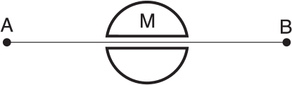
Figure 5: The straight path from $A$ to $B$ passes through mass $M$. With the mass in place, light takes longer to propagate from $A$ to $B$ than without the mass present, whereas a non-relativistic material particle travels from $A$ to $B$ faster with $M$ present than without. How can light be slowed and particles hastened along the same path in the same gravitational field?

Light propagating from $A$ to $B$ through the mass $M$ has its propagation time delayed from what it would be without the mass present, but a non-relativistic particle traveling the same path arrives at $B$ sooner than it would without the mass $M$ present. How can light be slowed and particles be hastened along the same path in the same gravitational field? In the SO-picture the answer is clear. The delay for light, as for radar, is due to the increased G-space distance between $A$ and $B$ when the mass $M$ is in place. The material particle must also travel the longer path between $A$ and $B$, but unlike the photon which experiences no gravitational acceleration in G-space ($\mathbf{g}=0$), a slow material particle experiences the Newtonian acceleration $\mathbf{g}_{0}=-\nabla\Phi$, which increases the particle’s speed as it nears and crosses the mass $M$, thus decreasing the travel time. Hence the particle arrives sooner and the photon later because the particle experiences a gravitational acceleration in G-space and the photon does not.

MO-Picture Interpretation: For comparison, we note that the acceleration due to gravity in MO-space (the absolute acceleration on the time scale of the coordinate time $\bar{t}$),

$$\bar{g}^{k} = \frac{d^{2}x^{k}}{d\bar{t}^{2}}+\bar{\Gamma}^{k}_{ij}\frac{dx^{i}}{d\bar{t}}\frac{dx^{j}}{d\bar{t}}$$ (36)

$$= -\frac{\partial\bar{\phi}}{\partial x_{k}}+\frac{1}{\bar{\phi}}\left(\frac{\partial\bar{\phi}}{\partial x^{i}}\frac{dx^{i}}{d\bar{t}}\right)\frac{dx^{k}}{d\bar{t}},$$

is not the gradient of a scalar potential alone, but in addition contains a velocity-dependent term that enforces the speed limit $d\bar{\ell}/d\bar{\tau}_{0}\leq c$ in MO-space [here $\bar{\Gamma}^{k}_{ij}=(1/2)\bar{g}^{kl}(\partial_{j}\bar{g}_{li}+\partial_{i}\bar{g}_{lj}-\partial_{l}\bar{g}_{ij})$ are the Christoffel symbols in MO-space and

$$\bar{\phi}=-\frac{1}{2}c^{2}\bar{g}_{00}$$ (37)

is the low-speed gravitational potential in this space].

There are two fundamental differences between the G-space equation of motion (22) and the Newtonian equation of motion (33). The first (a local difference) is the factor $(\bar{m}c^{2}/E)^{2}$ discussed above. The second difference (a global one) is the curvature of Gaussian space for equation (22) whereas the space for the Newtonian equation (33) is flat. In the following section we learn that this difference accounts for the perihelion precession of planetary orbits.

IV.3 Relativistic Kepler Problem

In Schwarzschild geometry (9), the “Newtonian gravitational potential” (23) for an observer at infinity is

$$\Phi=-\frac{GM}{r}+\frac{c^{2}}{2}.$$ (38)

Apart from the additive constant $c^{2}/2$, this is formally identical to the Newtonian gravitational potential for this problem [the additive constant is, of course, arbitrary in Newtonian theory, but fixed by equations (2) and (23) in the SO-picture of general relativity]. The gravitational acceleration in G-space, Eq. (35), reads

$$\mathbf{g}=\left(\frac{\bar{m}c^{2}}{E}\right)^{2}\nabla\left(\frac{GM}{r}\right).$$ (39)

The constant factor $(\bar{m}c^{2}/E)^{2}$ in this equation is equivalent to a change of the central mass $M$ by this factor; a change which is entirely negligible for planetary motions in the solar system (the change is less than one part in $10^{7}$ for planet Mercury in the sun’s field, and $M_{\odot}$ is known only to about four significant figures anyway). Moreover, a small change in the strength of the Newtonian inverse-square acceleration makes no contribution to the perihelion motion (such a change acting alone still gives closed elliptical orbits). Therefore, the precession of perihelion can only be attributed to the non-Euclidean character of G-space:

Result VII: In the single-observer picture, the relativistic precession of perihelion of planetary orbits is due exclusively to the curvature of Gaussian space.

Let us show this explicitly. In the $\theta=\pi/2$ plane of Schwarzschild space, we write the G-space metric, Eq.(11), as

$$d\ell^{2}=\frac{1}{(1-2m^{*}/r)}\left[\frac{dr^{2}}{(1-2m^{*}/r)}+r^{2}d\phi^{2}\right].$$ (40)

with a star on $m^{*}$ so that we can “turn off” the curvature of G-space by setting $m^{*}=0$, without changing the gravitational potential (38) [this is, of course, an artificial procedure, but one that allows us to isolate the effect of G-space curvature].

The orbit equation for the variable $u(\phi)=1/r(\phi)$ is derived from from the equation of motion (22) in the usual way. The result is

$$\frac{d^{2}u}{d\phi^{2}}+u=\frac{GM}{h^{2}}+3m^{*}u^{2},$$ (41)

where

$$h=\frac{r^{3}}{r-2m^{*}}\left(\frac{d\phi}{dt}\right)\approx r^{2}\frac{d\phi}{dt}$$ (42)

is a constant of the motion (the angular momentum per unit mass), and we have replaced $(\bar{m}c^{2}/E)^{2}$ by unity because the difference is negligible for any planetary motion in the solar system.

The first term on the right in (41) (the Newtonian term) comes from the potential (38), whereas the second term (the relativistic term) comes from the G-space metric (40) and gives rise to the observed advance of perihelion. But, if we turn off the curvature of G-space by setting $m^{*}=0$, equation (41) is then the Newtonian orbit equation with no precession of perihelion. In this sense the precession [$\delta\phi=6\pi m^{*}/a(1-\epsilon^{2})$ per revolution, where $a$ is the semi-major axis and $\epsilon$ the eccentricity of the orbit] is a direct measure of the curvature of G-space.

MO-Picture Interpretation: Interpretation of perihelion precession is more complicated in MO-spacetime. Will Will3 identifies three separate significant contributions to the perihelion precession (three significant terms in the PPN expansion): (1) curvature of MO-space, (2) a velocity dependent part of the gravitational force, and (3) a non-linear term proportional to the square of the gravitational potential; the relative contribution of these effects being coordinate dependent.

It is noteworthy that the single-observer interpretation attributes the perihelion advance to a single cause (the curvature of G-space) and this interpretation is exact rather than approximate.

V THE GRAVITATIONAL POTENTIAL IN GAUSSIAN SPACE

Let us derive the field equation for the “Newtonian gravitational potential”

$$\Phi=\frac{1}{2}c^{2}\mathcal{R}^{2}$$ (43)

in G-space. The exact result is surprisingly simple and familiar.

To begin, the metric $d\bar{s}^{2}$ in the MO-picture is written in terms of G-space variables as

$$d\bar{s}^{2}=\mathcal{R}^{2}ds^{2}=\mathcal{R}^{2}\left(-c^{2}dt^{2}+g_{ij}dx^{i}dx^{j}\right).$$ (44)

Hence the metric tensor in the MO-picture reads

$$\bar{g}_{00} = -\mathcal{R}^{2},$$

$$\bar{g}_{ij} = \mathcal{R}^{2}g_{ij},$$

$$\bar{g}_{0i} = \bar{g}_{i0}=0.$$ (45)

From this we construct the 00-component of the Ricci tensor in the MO-picture. The result,

$$\bar{R}_{00}=\frac{1}{2\mathcal{R}^{2}}\left[\frac{1}{\sqrt{g}}\frac{\partial}{\partial x^{k}}\left(\sqrt{g}g^{kl}\frac{\partial\mathcal{R}^{2}}{\partial x^{l}}\right)\right]=\frac{\nabla^{2}\Phi}{c^{2}\mathcal{R}^{2}},$$ (46)

is the left hand side of the Einstein equation

$$\bar{R}_{00}=8\pi G(\bar{T}_{00}-\bar{g}_{00}\bar{T}/2)/c^{4}.$$ (47)

To evaluate the right hand side of this equation in the SO-picture we need the conformal transformation law for the stress-energy tensor $\bar{T}_{\alpha\beta}$. The simple case of pressureless fluid ($\bar{T}^{\mu\nu}=\bar{\rho}_{0}\bar{U}^{\mu}\bar{U}^{\nu}$) determines this transformation law as follows. The transformation for the mass density in the rest frame of the fluid [which is $\bar{\rho}_{0}=d\bar{m}/(d\bar{\ell})^{3}$ in the MO-picture and $\rho_{0}=dm/(d\ell)^{3}$ in the SO-picture] is determined by the transformation laws for mass ($dm=\mathcal{R}d\bar{m}$) and length ($d\ell=d\bar{\ell}/\mathcal{R}$):

$$\rho_{0}=\mathcal{R}^{4}\bar{\rho}_{0}.$$ (48)

The transformation for the fluid four-velocity $\bar{U}^{\mu}$ [which is $\bar{U}^{\mu}=dx^{\mu}/d\bar{\tau}$ in the MO-picture and $U^{\mu}=dx^{\mu}/d\tau$ in the SO-picture] is determined by the transformation law for proper time ($d\bar{\tau}=\mathcal{R}d\tau$):

$$U^{\mu}=\mathcal{R}\bar{U}^{\mu}.$$ (49)

Hence the stress-energy tensor in the SO-picture, $T^{\mu\nu}\equiv\rho_{0}U^{\mu}U^{\nu}$, is related to the stress-energy tensor $\bar{T}^{\mu\nu}=\bar{\rho}_{0}\bar{U}^{\mu}\bar{U}^{\nu}$ of the MO-picture as

$$T^{\mu\nu}=\mathcal{R}^{6}\bar{T}^{\mu\nu},$$ (50)

and lowering indices with the metric, which transforms as $g_{\alpha\beta}=\bar{g}_{\alpha\beta}/\mathcal{R}^{2}$, gives $T_{\mu\nu}=\mathcal{R}^{2}\bar{T}_{\mu\nu}$ and $T=T^{\mu}_{\mu}=\mathcal{R}^{4}\bar{T}$. All of these conformal transformation rules are consistent with the general transformation rule derived in the Appendix. Finally, the 00-component of Einstein’s equation (47) becomes the field equation for the gravitational potential $\Phi$ in Gaussian space:

Result VIII: The acceleration due to gravity for a particle at rest in Gaussian space, $\mathbf{g}_{0}=-\nabla\Phi$, is derivable from a potential $\Phi$ which satisfies the same linear Poisson equation as in Newtonian gravitation theory,

$$\nabla^{2}\Phi=4\pi G\rho_{g},$$ (51)

with active gravitational mass density

$$\rho_{g}=(2T_{00}-g_{00}T)/c^{2}$$ (52)

acting as the source of gravitational field. This is the ultimate justification for calling $\Phi$ the “Newtonian gravitational potential”.

In view of this result, the equations for the “Newtonian gravitational field” $\mathbf{g}_{0}$ in G-space can be written as

$$\nabla\cdot\mathbf{g}_{0} = -4\pi G\rho_{g},$$

$$\nabla\times\mathbf{g}_{0} = 0.$$ (53)

The first of these, when integrated over a volume $V$ with closed surface $S$, gives the gravitational Gauss law in G-space:

Result IX: The flux of $\mathbf{g}_{0}$ through any closed surface $S$ in G-space equals $4\pi G$ times the total active gravitational mass $M_{g}$ inside the surface:

$$\oint_{S}\mathbf{g}_{0}\cdot d\mathbf{a}=4\pi GM_{g},$$ (54)

where

$$M_{g}=\int_{V}\rho_{g}\sqrt{g}d^{3}x.$$ (55)

This result follows because the divergence theorem holds true in a non-Euclidean three-space as well as a Euclidean one.

Result IX may be used to operationally define the mass $M_{g}$ inside a closed surface in G-space in terms of the field $\mathbf{g}_{0}$ on that surface (without the space being asymptotically flat), or to calculate the gravitational field $\mathbf{g}_{0}$ in cases of simple symmetry, just as the electric field is calculated using the electrostatic Gauss law in a flat space.

MO-Picture Interpretation For comparison, we note that the exact field equation for the “gravitational potential” $\bar{\phi}=-c^{2}\bar{g}_{00}/2$ in MO-space (the potential whose gradient $\bar{g}_{k}=-\partial\bar{\phi}/\partial x^{k}$ is the rest acceleration due to gravity in this space) is the 00-component of Einstein’s equation $\bar{R}_{\mu\nu}=(8\pi G/c^{2})(\bar{T}_{\mu\nu}-\bar{g}_{\mu\nu}\bar{T}/2)$, namely the non-linear equation

$$\bar{\nabla}^{2}\bar{\phi}-\frac{\bar{\nabla}\bar{\phi}\cdot\bar{\nabla}\bar{\phi}}{2\bar{\phi}}=4\pi G\bar{\rho}_{g},$$ (56)

where $\bar{\rho}_{g}=(2\bar{T}_{00}-\bar{g}_{00}\bar{T})/c^{2}$ is the density of active gravitational mass in MO-space. There do not appear to be any simple exact results in the MO-picture analogous to Results VIII and IX in SO-space.

The linear Poisson equation (51) for the gravitational potential $\Phi$ in G-space is an exact, fully relativistic result valid for any static gravitational field. This result is surprising because the Einstein equation, from which it is derived, is clearly non-linear.

VI ELECTRODYNAMICS

In MO-spacetime the electromagnetic field $\bar{F}_{\mu\nu}$ is governed by Maxwell’s equations

$$\bar{\nabla}_{\omega}\bar{F}_{\mu\nu}+\bar{\nabla}_{\nu}\bar{F}_{\omega\mu}+\bar{\nabla}_{\mu}\bar{F}_{\nu\omega}=0,$$ (57a)

and

$$\bar{\nabla}_{\nu}\bar{F}^{\mu\nu}=-\frac{4\pi}{c}\bar{J}^{\mu},$$ (57b)

where $\bar{J}^{\mu}=(c\bar{\rho},\bar{\mathbf{j}})/\sqrt{-\bar{g}_{00}}$ is the four-current density, determined by the charge density $\bar{\rho}$ and current density $\bar{\mathbf{j}}$ in MO-space and $\bar{\nabla}_{\omega}$ is the covariant derivative based on the MO-metric $\bar{g}_{\alpha\beta}$. The motion of a particle of charge $\bar{q}$ and mass $\bar{m}$ is described by the Lorentz equation of motion

$$\frac{d\bar{P}^{\mu}}{d\bar{\tau}}+\bar{\Gamma}^{\mu}_{\ \alpha\beta}\bar{P}^{\alpha}\frac{dx^{\beta}}{d\bar{\tau}}=\frac{\bar{q}}{c}{{\bar{F}}^{\mu}}_{\ \nu}\frac{dx^{\nu}}{d\bar{\tau}},$$ (58)

where $\bar{P}^{\mu}=\bar{m}dx^{\mu}/d\bar{\tau}$ is the four-momentum of the particle and $\bar{\tau}$ it’s proper time.

The Maxwell equations (57) are conformally invariant. By this is meant that, if under the conformal transformation $g_{\alpha\beta}=\bar{g}_{\alpha\beta}/\mathcal{R}^{2}$ the field tensor and current density transform as

$$F_{\mu\nu}=\bar{F}_{\mu\nu}$$ (59)

and

$$J^{\mu}=\mathcal{R}^{4}\bar{J}^{\mu},$$ (60)

respectively [or equivalently ${F^{\mu}}_{\nu}=\mathcal{R}^{2}{{\bar{F}}^{\mu}}_{\nu}$ (or $F^{\mu\nu}=\mathcal{R}^{4}\bar{F}^{\mu\nu}$) and $J_{\mu}=\mathcal{R}^{2}\bar{J}_{\mu}$], then, after the conformal transformation, Maxwell’s equations have the same four-space forms as before, namely

$$\nabla_{\omega}F_{\mu\nu}+\nabla_{\nu}F_{\omega\mu}+\nabla_{\mu}F_{\nu\omega}=0,$$ (61a)

and

$$\nabla_{\nu}F^{\mu\nu}=-\frac{4\pi}{c}J^{\mu},$$ (61b)

where $\nabla_{\nu}$ is the covariant derivative appropriate to the SO-metric $g_{\alpha\beta}$ and $J^{\mu}=(c\rho,\mathbf{j})$ is the four-current density in SO-spacetime.

The equation of motion (58) is not conformally invariant. In SO-spacetime the equation of motion reads

$$\frac{dP^{\mu}}{d\tau}+\Gamma^{\mu}_{\ \alpha\beta}P^{\alpha}\frac{dx^{\beta}}{d\tau}=-\frac{\partial V}{\partial x_{\mu}}+\frac{q}{c}{F^{\mu}}_{\nu}\frac{dx^{\nu}}{d\tau},$$ (62)

where $V(\mathbf{x})=m(\mathbf{x})c^{2}$ is the rest energy of the particle in this picture, and we have used ${F^{\mu}}_{\nu}=\mathcal{R}^{2}{{\bar{F}}^{\mu}}_{\nu}$, $d\tau=d\bar{\tau}/\mathcal{R}$, $P^{\mu}=\mathcal{R}^{2}\bar{P}^{\mu}$, and $q=\bar{q}$ in the derivation. The charges $q$ and $\bar{q}$ in the SO- and MO-pictures, respectively, are set equal to one another (as opposed to some other transformation law $q=\mathcal{R}^{s}\bar{q}$ with $s\neq 0$) so that the mere motion of a single charge does not violate charge conservation in the SO-picture. This also follows from the charge conservation law $\nabla_{\mu}J^{\mu}=0$ in SO-spacetime, which is derivable from (61b).

This completes the four-space formulation of classical electrodynamics in the SO-picture. But our interest here centers on the forms taken by Maxwell’s equations in the Gaussian three-space and how these compare with the corresponding equations in MO-space. As we shall see, the conformal invariance of the 4-space Maxwell equations does not imply that the 3-space Maxwell equations are the same in the MO- and SO-pictures because the metric elements $\bar{g}_{00}$ and $g_{00}$ ($=-1$) are different in the two pictures.

VI.1 Maxwell’s Equations in MO-Space

There have been several three-space (or “3+1”) formulations of Maxwell’s equations in the MO-picture, all of which seem to have certain “unphysical” features. Here we consider two of them.

Perhaps the earliest formulation is the one in which the electrodynamic equations in a static gravitational field are formally identical to the Maxwell equations in a material medium:

$$\bar{\nabla}\cdot\tilde{\mathbf{D}} = 4\pi\tilde{\rho},$$ (63a)

$$\bar{\nabla}\cdot\tilde{\mathbf{B}} = 0,$$ (63b)

$$\bar{\nabla}\times\tilde{\mathbf{H}}-\frac{1}{c}\frac{\partial\tilde{\mathbf{D}}}{\partial\bar{t}} = \frac{4\pi}{c}\tilde{\mathbf{j}},$$ (63c)

$$\bar{\nabla}\times\tilde{\mathbf{E}}+\frac{1}{c}\frac{\partial\tilde{\mathbf{B}}}{\partial\bar{t}} = 0,$$ (63d)

with constitutive relations

$$\tilde{\mathbf{D}} = \frac{\tilde{\mathbf{E}}}{\sqrt{-\bar{g}_{00}}}=\tilde{\epsilon}\tilde{\mathbf{E}},$$ (64)

$$\tilde{\mathbf{H}} = \frac{\tilde{\mathbf{B}}}{\sqrt{-\bar{g}_{00}}}=\frac{\tilde{\mathbf{B}}}{\tilde{\mu}},$$ (65)

corresponding to a medium with “dielectric constant” $\tilde{\epsilon}$ and “magnetic permeability” $\tilde{\mu}$ given by

$$\tilde{\epsilon}=\frac{1}{\tilde{\mu}}=\frac{1}{\sqrt{-\bar{g}_{00}}}.$$ (66)

In equations (63), $\bar{\nabla}\cdot\tilde{\mathbf{D}}$ and $\bar{\nabla}\times\tilde{\mathbf{E}}$ are the divergence and curl in MO-space (the three-space with metric $\bar{g}_{ij}$). Equations (63) are derived and studied in Landau and Lifshitz Landau . We shall refer to them as the “material Maxwell equations”.

It is pleasant that the Maxwell equations (63) take the familiar forms for electrodynamics in a material medium, but the interpretations of $\tilde{\epsilon}$ as a dielectric constant and of $\tilde{\mu}$ as a magnetic permeability of space are without physical foundation (empty space contains neither the electric charges to be a dielectric medium nor the electric currents to be a magnetic one). Moreover, the electric field $\tilde{\mathbf{E}}$ in the material Maxwell equations is not the electric field measured locally (it is more a formal field than a physical one). For these reasons, the material Maxwell equations must be viewed as “unphysical”.

An important step toward physical clarity was taken by Thorne and Macdonald Thorne1 and others Thorne2 , in connection with the membrane paradigm for black holes. In this approach, the electric and magnetic fields

$$\bar{E}^{k}=\frac{{\bar{F}}^{k}_{0}}{\sqrt{-\bar{g}_{00}}}=\frac{\tilde{E}^{k}}{\sqrt{-\bar{g}_{00}}}$$ (67)

and

$$\bar{B}^{k}=\frac{1}{2}\bar{e}^{k}_{ij}\bar{F}^{ij}=\tilde{B}^{k},$$ (68)

are those measured locally using the traditional time and length standards of the MO-picture. For these fields, the three-space Maxwell equations read

$$\bar{\nabla}\cdot\bar{\mathbf{E}} = 4\pi\bar{\rho},$$ (69a)

$$\bar{\nabla}\cdot\bar{\mathbf{B}} = 0,$$ (69b)

$$\frac{1}{c}\frac{\partial\bar{\mathbf{B}}}{\partial\bar{t}} = -\bar{\nabla}\times(\alpha\bar{\mathbf{E}}),$$ (69c)

$$\frac{1}{c}\frac{\partial\bar{\mathbf{E}}}{\partial\bar{t}} = \bar{\nabla}\times(\alpha\bar{\mathbf{B}})-\frac{4\pi}{c}\alpha\bar{\mathbf{j}},$$ (69d)

where $\alpha=\sqrt{-\bar{g}_{00}}$ is called the “lapse function,” and $\bar{\rho}$ ($=\tilde{\rho}$) and $\bar{\mathbf{j}}$ ($=\tilde{\mathbf{j}}/\sqrt{-\bar{g}_{00}}$) are the locally measured charge and current densities.

Equations (69) are not in the form of Maxwell’s equations for a material medium. However, they do ascribe electric and magnetic properties to empty space, e.g., the Schwarzschild surface behaves in many respects like a conducting membrane, and this is often useful, though in reality there are no electric currents in this surface.

It is desirable, for aesthetic as well as practical reasons, to have a three-space formulation of Maxwell’s equations that is “true to the physics” in the sense that it does not assign electric or magnetic properties to empty space where there are no charges or currents. In the next section we show that the SO-picture provides such a formulation.

VI.2 Maxwell’s Equations in Gaussian Space

In order to define electric and magnetic fields appropriate to the SO-picture, we multiply equation of motion (62) by $d\tau/dt=mc^{2}/E$ and note that, for the SO-metric (4), only the spatial components $\Gamma^{k}_{\ ij}$ of the Christoffel symbols $\Gamma^{\mu}_{\ \alpha\beta}$ are non-zero. The spatial components of the result are

$$\frac{Dp^{k}}{dt} \equiv \frac{dp^{k}}{dt}+\Gamma^{k}_{\ ij}p^{i}\frac{dx^{j}}{dt}$$ (70)

$$= -\left(\frac{mc^{2}}{E}\right)\frac{\partial V}{\partial x_{k}}+q\left({F^{k}}_{0}+\frac{v^{j}}{c}{F^{k}}_{j}\right),$$

and the time component reads

$$\frac{DP^{0}}{dt}=\frac{d}{dt}\left(\frac{E}{c}\right)=\frac{q}{c}F^{0}_{\ j}v^{j},$$ (71)

where $v^{j}\equiv dx^{j}/dt$, $p^{k}=mdx^{k}/d\tau$, $E=mc^{2}/\sqrt{1-v^{2}/c^{2}}$ (no longer a constant of the motion), and, as before, $m=\bar{m}\mathcal{R}$ and $q=\bar{q}$. Note that the “Newtonian gravitational three-force” $F^{k}_{G}=-(mc^{2}/E)\partial V/\partial x_{k}$ vanishes as the particle speed approaches $c$ (as $E/mc^{2}\rightarrow\infty$), and the electromagnetic three-force has the Lorentz form [$F^{k}=q(E^{k}+e^{k}_{\ ij}v^{i}B^{j}/c)$] if and only if the electric and magnetic fields in G-space are defined as

$$E^{k} \equiv {F^{k}}_{0}=\mathcal{R}^{3}\bar{E}^{k},$$ (72)

$$B^{k} \equiv \frac{1}{2}e^{k}_{\ ij}F^{ij}=\mathcal{R}^{2}\bar{B}^{k},$$ (73)

and so

$$E_{i} = g_{ij}E^{j}=F^{0}_{\ \ i},$$ (74)

$$F^{i}_{\ j} = e^{i\ k}_{\ j}B_{k},$$ (75)

where $e_{kij}$ is the permutation tensor in G-space [$e_{kij}=\sqrt{g}\epsilon_{kij}$ and $e^{k}_{\ ij}=g^{kl}e_{lij}$, where $\epsilon_{ijk}$ is the permutation symbol and $g=det(g_{ij})$]. Thus we have

Result X: The equations of motion in Gaussian space read

$$\frac{d\mathbf{p}}{dt}=-\left(\frac{mc^{2}}{E}\right)\nabla V+q\left(\mathbf{E}+\frac{\mathbf{v}}{c}\times\mathbf{B}\right),$$ (76)

$$\frac{dE}{dt}=q\mathbf{E}\cdot\mathbf{v},$$ (77)

where $d\mathbf{p}/dt$ is the absolute derivative in G-space of the three-momentum $\mathbf{p}=m\mathbf{v}/\sqrt{1-v^{2}/c^{2}}$ and the electric and magnetic fields in Gaussian space, $\mathbf{E}$ and $\mathbf{B}$, are related to the electric and magnetic fields $\bar{\mathbf{E}}$ and $\bar{\mathbf{B}}$ measured locally in MO-space by the conformal transformations

$$\mathbf{E} = \mathcal{R}^{3}\bar{\mathbf{E}},$$ (78)

$$\mathbf{B} = \mathcal{R}^{2}\bar{\mathbf{B}}.$$ (79)

The gravitational force $\mathbf{F}_{G}=-(mc^{2}/E)\nabla V$ in Gaussian space tends to zero as $v\rightarrow c$ because $E\rightarrow\infty$ in this limit.

Just as $\bar{\mathbf{E}}$ and $\bar{\mathbf{B}}$ are the locally measured fields in MO-space (measured using length and time standards based on a local free-running atomic clock), $\mathbf{E}$ and $\mathbf{B}$ are locally measured fields in the SO-picture (measured using time and length standards based on a local clock that is slaved to our single-observer’s clock by time signals). Thus $\mathbf{E}$ and $\mathbf{B}$ are the physically correct local fields in the view of our self-centered observer (the fields are “corrected” for time and space dilation at the location under consideration). Using (78) and (79) in equations (69) and expanding those equations in terms of G-space variables (specifically going over to G-space covariant derivatives in place of MO-space ones), we obtain the Maxwell equations in G-space:

Result XI: The Maxwell equations in Gaussian space,

$$\nabla\cdot\mathbf{E} = 4\pi\rho,$$ (80a)

$$\nabla\cdot\mathbf{B} = 0,$$ (80b)

$$\nabla\times\mathbf{B}-\frac{1}{c}\frac{\partial\mathbf{E}}{\partial t} = \frac{4\pi}{c}\mathbf{j},$$ (80c)

$$\nabla\times\mathbf{E}+\frac{1}{c}\frac{\partial\mathbf{B}}{\partial t} = 0,$$ (80d)

are formally identical to the Maxwell equations in the absence of a gravitational field; the only difference being the divergence and curl in these equations are the ones appropriate to the non-Euclidean G-space metric $g_{ij}$ instead of the flat-space metric of classical physics. The charge and current densities in Gaussian space are expressed in terms of those measured locally in the MO-picture by the conformal transformation laws

$$\rho = \mathcal{R}^{3}\bar{\rho},$$ (81)

$$\mathbf{j} = \mathcal{R}^{4}\bar{\mathbf{j}}.$$ (82)

The charge and current densities in G-space, equations (81) and (82), are the physically correct ones in the view of our single observer: $\rho$ is the charge per unit volume as measured with the single-observer length standard and $\mathbf{j}$ is $\rho$ times the velocity of this charge measured using single-observer time $t$.

Equations (80a)-(80d) show that, in G-space, the dielectric constant and magnetic permeability of the vacuum are unity everywhere ($\bar{\epsilon}=\bar{\mu}=1$), and there are no fictitious electric or magnetic properties of empty space in this picture.

VI.3 Gauss’ law, Faraday’s law, and Ampere’s law in Gaussian Space

In the non-Euclidean G-space the integral theorems of Gauss and Stokes’ apply in there usual forms:

$$\int_{V}\nabla\cdot\mathbf{W}dv=\oint_{S}\mathbf{W}\cdot d\mathbf{a},$$ (83)

$$\int_{S}(\nabla\times\mathbf{W})\cdot d\mathbf{a}=\oint_{C}\mathbf{W}\cdot d\mathbf{l},$$ (84)

where $\mathbf{W}$ is any well behaved vector field, $V$ is a volume in G-space (with volume element $dv=\sqrt{g}d^{3}x$) bounded by the closed surface $S$ in (83). In Eq. (84) $S$ is an open surface with area element $d\mathbf{a}$ bounded by the closed contour $C$ with displacement element $d\mathbf{l}$ along the contour.

Applying these theorems to the Maxwell equations (80), we obtain the integral forms of Maxwell’s equations in G-space:

$$\oint_{S}\mathbf{E}\cdot d\mathbf{a} = 4\pi\int_{V}\rho dv,$$ (85a)

$$\oint_{S}\mathbf{B}\cdot d\mathbf{a} = 0,$$ (85b)

$$\oint_{C}\mathbf{E}\cdot d\mathbf{l} = -\frac{1}{c}\frac{d}{dt}\int_{S}\mathbf{B}\cdot d\mathbf{a},$$ (85c)

$$\oint_{C}\mathbf{B}\cdot d\mathbf{l} = \frac{4\pi}{c}\int_{S}\mathbf{j}\cdot d\mathbf{a}+\frac{1}{c}\frac{d}{dt}\int_{S}\mathbf{E}\cdot d\mathbf{a},$$ (85d)

Thus we have the following electromagnetic laws in Gaussian space which are familiar from flat-space electrodynamics:

Result XII (Gauss’ Law): The flux of the electric field through any closed surface in G-space is $4\pi$ times the total charge inside the surface.

Result XIII (No Magnetic Monopoles): The flux of the magnetic field through any closed surface in G-space is zero.

Result XIV (Faraday’s Law): The electromotive force (the line integral of $\mathbf{E}$ around the closed contour $C$) is $-1/c$ times the rate of change of the flux of $\mathbf{B}$ through any surface $S$ having the contour $C$ as edge.

Result XV (Ampere’s Law): The line integral of $\mathbf{B}$ around a closed contour $C$ equals $4\pi/c$ times the total current passing through the contour, including the displacement current

$$I_{D}=\frac{1}{4\pi}\frac{d}{dt}\int_{S}\mathbf{E}\cdot d\mathbf{a}.$$ (86)

These results imply that Faraday’s picture of electric and magnetic field lines is applicable in G-space. As in flat space, these laws are useful for the calculation of electric and magnetic fields when the symmetry of the problem is simple. The only substantive change is that lengths of contours and areas of surfaces are calculated using the non-Euclidean G-space metric instead of the flat-space metric of classical electrodynamics.

MO-Picture Interpretation: It is important to note that, generally speaking, Results XII through XV do not hold true in MO-space:

• Result XII implies that electric field lines in G-space start on positive charges, end on negative charges, or go off to spatial infinity (if such exits). That is to say, electric field lines do not start or end in empty space [this is not the case in MO-space where electric field lines can begin or end in empty space due to an inhomogeneous dielectric constant of the vacuum].

• Result XIII states that magnetic field lines neither begin nor end in G-space. This means, as in Euclidean space, that either magnetic field lines form closed loops or else they go off to spatial infinity (if such exits) [this result does not apply in MO-space where an inhomogeneous permeability of empty space can cause magnetic field lines to begin or end in vacuum].

• Result XIV, Faraday’s Law, applies in MO-space as well as G-space when we employ the material Maxwell equations (57), but does not apply in MO-space when using the Maxwell equations for locally measured fields (69).

• Result XV, Ampere’s Law with displacement current, does not apply in MO-space for either the material Maxwell equations (57) or the Maxwell equations for locally measured fields (69).

VII A POSSIBLE DIRECT TEST OF GRAVITATIONAL SPACE DILATION

The formalism of gravitational space dilation is based on the scaling laws

$$d\tau = \frac{d\bar{\tau}}{\mathcal{R}},$$ (87a)

$$d\ell = \frac{d\bar{\ell}}{\mathcal{R}},$$ (87b)

relating the locally measured time $d\bar{\tau}$ and length $d\bar{\ell}$ to the time $d\tau$ and length $d\ell$ measured by a distant observer $O$. As noted earlier, Eq. (87a) has been well tested in gravitational time dilation experiments.

In the present section we show that, in principle, space dilation [Eq. (87b)] can also be measured directly, and that a solar-system test of space dilation seems to be within the capability of current technology.

But hasn’t space dilation already been tested in the relativistic radar echo delay experiment? Placing the sun’s mass near the radar propagation path increases the length of that path in Gaussian space and this nicely accounts for the additional radar delay. Isn’t this a direct test of gravitational length dilation? The answer to these questions is in the negative. The radar delay experiment measures the difference in radar path length (G-space distance) with the sun “near to” and “far from” the radar propagation path, whereas the space dilation formula (87b) relates the proper lengths $d\bar{\ell}$ and $d\ell$ of a single spatial interval measured by local and distant observers (the proper lengths in the MO- and SO-pictures, respectively) in a single fixed gravitational field. These are quite different concepts and should not be confused. To test the space dilation formula (87b) one must measure $d\bar{\ell}$ and $d\ell$ independently and then determine whether or not these results are related by equation (87b). Fortunately, the two lengths $\bar{\ell}$ and $\ell$ (they are, of course, finite in any experiment) can both be measured by means of radar. The MO-picture proper length $\bar{\ell}$ is the radar distance measured locally by a radar located, say, at one end of the interval $\bar{\ell}$ with a transponder at the other end (we assume that the gravitational potential is essentially constant over this length). And, as shown in Sec. III, the SO-proper length $\ell$ of the same spatial interval is measured by a radar located at our distant observer $O$, perhaps using transponders at both ends of the interval $\bar{\ell}$ (or $\ell$)

In a solar-system experiment this might be accomplished as depicted in Fig. 6.

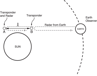
Figure 6: Spacecraft $A$ uses radar to locally measure the distance $\bar{\ell}$ to spacecraft $B$ in the sun’s gravitational field and transmits this information to Earth. This is the proper distance in the MO-picture. Observer $O$ on Earth uses radar to measure the same displacement $AB$ from his distant location and obtains the dilated value $\ell=\bar{\ell}/\mathcal{R}$. In this way the space-dilation formula (87b) may be tested, at least in principle and perhaps in practice.

Two spacecraft, $A$ and $B$, orbit the sun with proper distances $\bar{\ell}$ and $\ell$ between them in the MO- and SO-pictures, respectively. $A$ and $B$ are equipped with radar transponders and $A$ also has an on-board radar for measuring the distance $\bar{\ell}$ to $B$, and a radio transmitter for sending this information to Earth. At the moment under consideration, $A$, $B$, and Earth lie on a G-space geodesic (a light ray) so that radar from earth measures the G-space distance $\ell$ directly. In this way $\bar{\ell}$ and $\ell$ for the interval $AB$ are independently measured and one can check that the space dilation formula $\ell=\bar{\ell}/\mathcal{R}$ is satisfied.

This is, of course, an extremely idealized experiment. In practice, the spacecraft $A$ and $B$ would not be lined up so neatly, and the Earth-based observer would measure the projection $\ell cos\theta$ of the length $\ell$ onto his line of sight, requiring knowledge of the angle $\theta$ between $AB$ and the line $OA$ extended (presumably this could be obtained from orbital calculations). Then there is the problem of the motions of $A$, $B$, and Earth during the propagation of radar pulses, and so on. Therefore, our description of the experiment is very crude indeed. Nevertheless, an order-of-magnitude estimate based on the accuracy achieved in passed radar delay experiments suggests that such an experiment might be within the capability of existing technology.

VIII APPLICATIONS

In this section we apply the single-observer formalism to a number of simple problems chosen to emphasize how very different physical interpretations can be in the MO- and SO-pictures.

VIII.1 Photon Frequency

In the MO-picture, an electromagnetic wave (or photon) propagating from point $A$ to point $B$ in a static gravitational field experiences a change in frequency from $\bar{f}_{A}$ to $\bar{f}_{B}$ described by the gravitational red-shift formula

$$\frac{\bar{f}_{A}}{\bar{f}_{B}}=\frac{\mathcal{R}(A)}{\mathcal{R}(B)}=\sqrt{\frac{\bar{g}_{00}(A)}{\bar{g}_{00}(B)}}.$$ (88)

The fundamental scaling law $\tau=\bar{\tau}/\mathcal{R}$ for time intervals from the MO-picture to the SO-picture implies the scaling law $f=\mathcal{R}\bar{f}$ for frequencies. Hence the gravitational red-shift relation (88) becomes

$$f_{A}=f_{B}$$ (89)

in Gaussian space (these are the frequencies measured with slave-clock time standards at $A$ and $B$).

Result XVI: In the SO-picture, the frequency and wavelength of an electromagnetic wave (or photon) are unchanged by propagation in a static gravitational field.

In G-space the wavelength $\lambda=c/f$ is also unchanged because $c$ and $f$ are unchanged (our single observer holds the view that the frequency shift in the MO-picture is a spurious effect resulting from the use of local time standards that run at different rates at different points in the gravitational field, as opposed to using a single global time that increases at the same rate everywhere).

Because the photon frequency $f$ is unchanged by propagation in the SO-picture, the photon energy $E=hf$ is also unchanged. The relevant conformal transformation laws are $f=\mathcal{R}\bar{f}$, $h=\bar{h}$, and $E=\mathcal{R}\bar{E}$, i.e., Plank’s constant is the same in the two pictures (see Appensix A for a derivation). The gravitational “red shift” in the SO-picture is attributed to a change in atomic rest energy with position [$mc^{2}=\bar{m}\mathcal{R}(\mathbf{x})c^{2}$]. Each energy level of the atom changes in this way with position and, therefore, an atomic transition that is in resonance with light of frequency $f$ at one point of space will not be in resonance with the same light wave when moved to a different location. The change in an atomic energy level is the work done in lifting the atom (quasistatically) against the “Newtonian gravitational force” $\mathbf{F}=-\nabla V=-\nabla(mc^{2})$. Hence, in the SO-picture, there is no “gravitational red shift of light” but instead a shift of atomic energy levels $E_{n}=m_{n}c^{2}$. In the SO-picture, the position-dependent energy levels of the atom $E_{n}(\mathbf{x})$ show themselves in two ways: (1) the principle of virtual work tells us that an atom in state $n$ experiences a gravitational force $\mathbf{F}=-\nabla E_{n}$, and (2) the change in atomic transition frequencies $\omega_{nm}=(E_{n}-E_{m})/\hbar$ accounts for the gravitational “red shift” observations.

VIII.2 Falling Toward a Black Hole

Consider a particle falling radially inward from rest at $r=\infty$ to a spherical black hole of Schwarzschild radius $r_{s}=2m$. At radial coordinate $r$ it’s inward velocity on the time scale of a distant observer (proper distance $d\bar{\ell}$ traveled in coordinate time $d\bar{t}$) is

$$\bar{v}_{r}=-\frac{d\bar{\ell}}{d\bar{t}}=\sqrt{\frac{2mc^{2}}{r}\left(1-\frac{2m}{r}\right)}.$$ (90)

This well-known result in the MO-picture states that the speed of the falling particle first increases and then tends to zero as $r\rightarrow 2m$ in such a way that the particle never crosses the Schwarzschild sphere at $r=2m$. It hovers just outside of this sphere indefinitely. In fact, the acceleration of the particle on this time scale,

$$\bar{g}_{r}=\frac{d\bar{v}_{r}}{d\bar{t}}=\frac{mc^{2}}{r^{2}}\left(\frac{4m}{r}-1\right)\sqrt{1-\frac{2m}{r}},$$ (91)

is radially outward ($\bar{g}_{r}>0$) for $r<4m$! It is this “repulsive gravitational acceleration” that slows the particle and prevents it from crossing the Schwarzschild sphere. Such is the accepted description of falling-particle motion for a distant observer in the MO-picture. It is a counter intuitive description if our intuition tells us that the gravitational acceleration ought always to be inward.

In the SO-picture, the speed of the falling particle increases monotonically on the time scale $t=\bar{t}$ of the observer at infinity,

$$v_{r}=-\frac{d\ell}{dt}=-\sqrt{\frac{2mc^{2}}{r}},$$ (92)

fortuitously having the same form as in Newtonian mechanics, with no outward gravitational acceleration (the velocity increases to $v_{r}=c$ at $r=2m$). How can this velocity of fall possibly be consistent with the distant observer’s observation that the particle never reaches the Schwarzschild surface? The answer is that, whereas the proper distance from any initial radial coordinate $r=r_{0}$ to $r=2m$, namely

$$\bar{\ell}=\int_{2m}^{r_{0}}d\bar{\ell}=\int_{2m}^{r_{0}}\frac{dr}{\sqrt{1-2m/r}},$$ (93)

is finite in the MO-picture, the same interval ($2m$, $r_{0}$) has infinite proper length

$$\ell=\int_{2m}^{r_{0}}d\ell=\int_{2m}^{r_{0}}\frac{dr}{1-2m/r}=\infty$$ (94)

in the SO-picture. So the particle never reaches the Schwarzschild surface in the SO-picture simply because the G-space distance to that surface is infinitely great. This conclusion is consistent with radar measurements made from any finite radial coordinate $r=r_{0}$. Because proper distance in the SO-picture is radar distance, the radar distance to the falling particle increases without bound as the particle approaches $r=2m$, and there is never a radar return from the Schwarzschild sphere, as one would expect for an infinitely distant object.

VIII.3 Propagation of Photon Polarization

In local Cartesian coordinates at an arbitrary point of G-space, the Maxwell equations (80) are identical in form to the vacuum Maxwell equations in flat space with rectangular coordinates. In these coordinates, light travels along straight lines at speed $c$ (at least in geometrical-optics approximation), and straight-line propagation in local Cartesian coordinates is equivalent to geodesic propagation in G-space. Hence, in the SO-picture, light is bent only by the curvature of G-space and not by the fictitious dielectric or magnetic properties of the vacuum (these contribute to the light deflection when analyzed using Maxwell’s equations in the MO-picture).

To say that light rays follow geodesics of G-space is to say that the tangent unit vector to the ray $\hat{\mathbf{k}}$ is parallel propagated along the ray. The unit electric polarization vector $\hat{\mathbf{e}}$ of a linearly polarized light ray, e.g., a laser beam, also undergoes parallel transport along the ray because it is unchanged by propagation in local Cartesian coordinates, and so does the magnetic polarization vector $\hat{\mathbf{b}}$, which is orthogonal to the other two unit vectors. Therefore we have

Result XVII: The tangent unit vector $\hat{\mathbf{k}}$, the electric polarization unit vector $\hat{\mathbf{e}}$, and the magnetic polarization unit vector $\hat{\mathbf{b}}$ of a linearly polarized light ray form an orthonormal set of three-vectors all of which undergo parallel transport along the ray in Gaussian space.

In MO-space there does not appear to be any comparably simple three-vector picture of the propagation of polarization.

VIII.4 Interferometry in a Gravitational Field

Light beams from a coherent source $S$ travel two distinct paths (path $A$ and path $B$) in a static gravitational field to the point $P$ where they interfere. The intensity of interference at $P$ depends on the phase difference of the two beams arriving there. Because wavelength $\lambda$ is constant along a ray in the SO-picture, the phase accumulated in propagating from $S$ to $P$ is proportional to the path length $\ell$ in this picture ($\phi=2\pi\ell/\lambda$). Thus the phase difference of the interfering beams, $\Delta\phi=2\pi(\ell_{A}-\ell_{B})/\lambda$, is determined by the path length difference $\ell_{A}-\ell_{B}$ in G-space. [In MO-space the wavelength changes as the light propagates and the calculation of phase difference is a bit more complicated, and the result is not proportional to the proper path length difference $\bar{\ell}_{A}-\bar{\ell}_{B}$].

VIII.5 What You Calculate is What You See

We should emphasize that the single-observer picture describes that which the single observers sees directly [“What You Calculate Is What You See” (WYCIWYS)]. The effects of spacetime dilation are already included in the formalism, and it is not necessary to correct for these effects at the end of a calculation, as sometimes must be done in the MO-picture when translating locally calculated results for comparison with observation from a distance. A couple of examples will clarify this point.

Suppose the local observer at $P$ measures a magnetic field $\bar{B}$ and constructs a simple clock by placing electrons in this field which, according to the Lorentz force law, orbit at the cyclotron frequency $\bar{\omega}_{c}=e\bar{B}/\bar{m}_{e}$. For the distant observer at $O$, Eq. (79) indicates the magnetic field is $B=\mathcal{R}^{2}\bar{B}$, and the mass of the electron for this observer is $m_{e}=\mathcal{R}\bar{m}_{e}$ (the charge is the same in both pictures: $q=\bar{q}=e$). Using the same Lorentz force law, observer $O$ calculates cyclotron frequency

$$\omega_{c}=\frac{eB}{m_{e}}=\frac{e\mathcal{R}^{2}\bar{B}}{\bar{m}_{e}\mathcal{R}}=\mathcal{R}\bar{\omega}_{c},$$ (95)

which is the red shifted frequency seen by this observer.

If our single observer uses Maxwell equations in G-space to calculate electromagnetic phenomena, the results of the calculations are automatically time-scaled to what he observes (WYCIWYS). No additional correction for spacetime dilation is necessary (there is, of course, a retardation delay in observing the result due to the finite light propagation speed).

As a second example, consider the transition frequencies of the Schrödinger hydrogen atom, which for the local observer are

$$\bar{\omega}_{nm}=\frac{\bar{m}_{e}\bar{e}^{4}}{2\bar{\hbar}^{3}}\left(\frac{1}{m^{2}}-\frac{1}{n^{2}}\right).$$ (96)

The charge, mass, and Plank constant scale to the SO-picture as $e=\bar{e}$, $m_{e}=\mathcal{R}\bar{m}_{e}$, and $\hbar=\bar{\hbar}$, respectively. Hence, using the same Schrödinger equation, observer $O$ calculates transition frequencies

$$\omega_{nm}=\frac{m_{e}e^{4}}{2\hbar^{3}}\left(\frac{1}{m^{2}}-\frac{1}{n^{2}}\right)=\mathcal{R}\bar{\omega}_{nm},$$ (97)

in agreement with the gravitational red-shift formula, but only if the photon frequency does not change while propagating in Gaussian space, as deduced earlier in this section.

VIII.6 Thermodynamic Equilibrium in Gaussian Space

It is a fundamental result of classical thermodynamics that two systems in thermal contact are in thermal equilibrium when their temperatures (among other things) are equal. For example, the atmosphere of a planet in thermal equilibrium has constant temperature throughout.

It is surprising, therefore, to learn that, in general relativity, this in not the case. In Tolman’s classic volume Tolman , we find that thermal equilibrium for a static fluid sphere held together by gravity is characterized by a position-dependent temperature $\bar{T}(\mathbf{x})$,

$$\frac{\bar{T}(\mathbf{x})}{\bar{T}(\mathbf{x}_{0})}=\sqrt{\frac{\bar{g}_{00}(\mathbf{x}_{0})}{\bar{g}_{00}(\mathbf{x})}}=\frac{1}{\mathcal{R}(\mathbf{x})},$$ (98)

where $\bar{T}(\mathbf{x}_{0})$ is the temperature at the position $\mathbf{x}_{0}$ of observer $O$. This means, for example, that the temperature of an equilibrium atmosphere in Schwarzschild geometry is larger the closer we are to the Schwarzschild surface at $r=2m$. This is thermal equilibrium in the MO-picture.

The equilibrium temperature distribution in the SO-picture is different from that in the MO-picture. To determine the conformal transformation law for temperature, we first note that the number of states accessible to a system $\Omega$, or the “disorder” of the system, as measured by the entropy

$$S=-k_{B}\sum_{n}P_{n}lnP_{n}=k_{B}ln\Omega$$ (99)

is clearly independent of the time and length standards chosen by an observer. Therefore the Boltzmann constant must be the same in the MO and SO pictures,

$$k_{B}=\bar{k}_{B}.$$ (100)

Then the quantity $k_{B}T$, with dimensions of energy, necessarily transforms as

$$k_{B}T=\mathcal{R}(\bar{k}_{B}\bar{T}),$$ (101)

(see Appendix A for justification) and, in view of (100), the transformation law for temperature reads

$$T=\mathcal{R}\bar{T}.$$ (102)

Thus, recalling that $\mathcal{R}(\mathbf{x}_{0})=1$, the condition for thermal equilibrium, Eq. (98), transformed to the SO-picture becomes the following result.

Result XVIII: A simple one-component fluid in hydrostatic equilibrium is in thermal equilibrium when its temperature, in the SO-picture, is constant throughout the fluid.

This result is in marked contrast to the MO-picture result (98), where thermal equilibrium is characterized by a higher temperature at lower gravitational potential. The SO-picture returns constant temperature to its classical role as determiner of thermal equilibrium.

The equilibrium atmosphere presents a clear example of the “What You Calculate Is What You See” (WYCIWYS) principle of the SO-picture. A black body at a point $P$ of low gravitational potential and in thermal equilibrium with an atmosphere at temperature $T$, radiates as a black body of this temperature according to observer $O$ who measures the spectrum of the radiation received from the body at $P$, and concludes it is at the same temperature as the atmosphere at his location.

The conventional relativist using the MO-picture disagrees with this conclusion. He believes that the black body at $P$ and the atmosphere at that location are hotter than the atmosphere at $O$, because $P$ is at lower gravitational potential and the system is in thermal equilibrium. He explains observer $O$’s observations by noting that the radiation of the hot black body at $P$ is redshifted as it propagates from $P$ to $O$, and so it only appears that the black body at $P$ has the same temperature as the atmosphere at $O$. This argument does not impress the self-centered observer at $O$ because, in his SO-picture, he knows of no such effect as the gravitational redshift of light. He knows only of a shift of atomic energy levels in a gravitational field.

The two pictures are physically equivalent and make the same predictions for the result of any measurement. The pictures differ only in the position-dependent length and time standards chosen to make the measurements.

IX SUMMARY AND CONCLUSION

The notion of gravitational space dilation derives from a single observer’s view that, when a distant observer’s standard time interval is dilated by a gravitational field, his standard length must be dilated as well and by the same factor. If this were not so, the distant observer could not understand how the local observer obtains the invariant value $c$ for the locally measured light speed. The single observer, making “corrections” for time and space dilation by means of a conformal transformation [$g_{\alpha\beta}=\bar{g}_{\alpha\beta}/\mathcal{R}^{2}$ with $\mathcal{R}^{2}=\bar{g}_{00}(P)/\bar{g}_{00}(O)$], arrives at the single-observer picture explored in this paper.

Perhaps the best way to summarize the qualitative results and equations of the single-observer picture is to compare these with the corresponding results and equations of classical (pre general relativity) physics. The similarities are striking:

• In the single-observer picture, as in Newtonian physics, gravitation is represented by a force. The gravitational acceleration $\mathbf{g}_{0}=-\nabla\Phi$ of non-relativistic particles ($v<<c$ or $E\approx\bar{m}c^{2}$) is derivable from a potential $\Phi$ that obeys the same linear Poisson equation,

  $$\nabla^{2}\Phi=4\pi G\rho_{g},$$ (103)

  as in Newtonian theory (an exact fully relativistic result).

• In Gaussian space, as in the classical Euclidean space, the electromagnetic three-force takes the Lorentz form,

  $$\mathbf{F}=q\left(\mathbf{E}+\frac{\mathbf{v}}{c}\times\mathbf{B}\right),$$ (104)

  with electric and magnetic fields that obey the vacuum Maxwell equations

  $$\nabla\cdot\mathbf{E}=4\pi\rho,$$ (105a)

  $$\nabla\cdot\mathbf{B}=0,$$ (105b)

  $$\nabla\times\mathbf{B}-\frac{1}{c}\frac{\partial\mathbf{E}}{\partial t}=\frac{4\pi}{c}\mathbf{j},$$ (105c)

  $$\nabla\times\mathbf{E}+\frac{1}{c}\frac{\partial\mathbf{B}}{\partial t}=0,$$ (105d)

  of the same form as in Maxwell’s original flat-space theory (an exact relativistic result).

• In Gaussian space, as in the classical three space, light rays propagate along geodesics of the three-space geometry and the frequency of light is unaffected by propagation in a static gravitational field.

• In the single-observer picture, the energy, momentum, and Lagrangian for a particle in a static gravitational field,

  $$E = \frac{mc^{2}}{\sqrt{1-v^{2}/c^{2}}},$$ (106)

  $$\mathbf{p} = \frac{m\mathbf{v}}{\sqrt{1-v^{2}/c^{2}}},$$ (107)

  $$L = -mc^{2}\sqrt{1-v^{2}/c^{2}},$$ (108)

  have the same forms as for a free particle in special relativity.

• As in classical physics, thermal equilibrium in the single-observer picture is characterized by uniform temperature.

These results justify our referring to the single-observer picture as the “classical picture” in general relativity. It is far closer in spirit to classical physics than the usual many-observer picture that is traditionally used in general relativity. Of course, the latter picture is not at all incorrect in its predictions (the two pictures are physically equivalent), but the classical picture is likely to be of interest to those who prefer to lean on their classical intuition when interpreting the results of general relativity.

There are, of course, differences between the “classical picture” in general relativity and classical physics prior to general relativity:

• In the classical picture, the rest mass $m=\bar{m}\mathcal{R}(\mathbf{x})$ and the rest energy $E=mc^{2}$ of a particle are position dependent in a gravitational field. The rest energy is the gravitational potential energy in this picture, and it’s gradient is the gravitational force.

  The position dependence of the rest energies $E_{n}=m_{n}(\mathbf{x})c^{2}$ of an atom (the atomic energy levels) shows itself through the position-dependent transition frequencies $\omega_{nm}=(E_{n}-E_{m})/\hbar$ which account for the “gravitational redshift” of spectral lines (if the rest masses of particles were not position-dependent, cyclotron clock frequencies and atomic transition frequencies would not correctly display the gravitational time dilation effect in this picture).

• When a particle moves fast ($v\sim c$ or $E>\bar{m}c^{2}$) it’s acceleration in Gaussian space,

  $$\mathbf{g}=\left(\frac{\bar{m}c^{2}}{E}\right)^{2}\mathbf{g}_{0},$$ (109)

  decreases from the Newtonian value $\mathbf{g}_{0}=-\nabla\Phi$ by the factor $(\bar{m}c^{2}/E)^{2}$ and approaches zero (geodesic motion in Gaussian space) as $E\rightarrow\infty$. Thus slow particles experience the Newtonian gravitational acceleration $\mathbf{g}_{0}$, but ultra-relativistic particles (and the photon) experience no acceleration and travel on geodesics of Gaussian space.

• Perhaps most importantly, Gaussian space is curved (non-Euclidean), whereas the three-space of classical physics is flat. In the single-observer picture, three of the four classic tests of general relativity are attributed to the curvature of Gaussian space. In this picture, the precession of perihelia, the bending of light by the sun’s gravitational field, and the relativistic radar echo delay are all measures of the curvature of the the solar G-space, and these interpretations are exact and complete (as opposed to an interpretation based on a limited number of terms in a perturbation expansion). This economy of interpretation seems desirable.

Another striking feature of the single-observer picture is the independence of all electromagnetic phenomena, from the Newtonian gravitational field $\mathbf{g}_{0}=-\nabla\Phi$! Electric and magnetic fields are “distorted” from their classical values by the non-Euclidean G-space geometry (and possibly by a non-classical topology of this space), but neither the potential $\Phi$ nor it’s gradient $\mathbf{g}_{0}=-\nabla\Phi$ appear in the Maxwell equations (105) in G-space, and consequently these have no affect on the fields $\mathbf{E}$ and $\mathbf{B}$ for any prescribed G-space metric $g_{ij}$. This is perhaps most clearly evident in local Cartesian coordinates where slow material particles fall with acceleration due to gravity $\mathbf{g}_{0}=-\nabla\Phi$, but the Maxwell equations (105) generate and propagate electric and magnetic fields in exactly the same manner as when $\mathbf{g}_{0}=0$. This result seems to be at variance with Einstein’s original principle-of-equivalence argument for the bending of light by the “gravitational field” in an upward accelerating elevator. But we must remember that Einstein’s argument gives only half the correct light deflection in the sun’s gravitational field, as in Einstein’s calculation Einstein1 prior to general relativity. In the SO-picture, no part of the light deflection is attributed to the principle of equivalence in this way. The deflection is entirely due to the curvature of the Gaussian three-space.

Finally, it is noteworthy that, in Gaussian space, the results of calculations made with the Maxwell equations or particle equations of motion for phenomena at some distance from the observer $O$ require no correction for gravitational time dilation at the location of the phenomena. The temporal scale of happenings anywhere in Gaussian space is as observed from $O$ (with, of course, a retardation delay due to the finite propagation speed $c$ of the optical image from phenomenon to observer); the correction for gravitational time dilation being already included in the formalism by means of the conformal transformation.

The results of the present paper (Part I) are limited to static gravitational fields. In a second paper (Part II) we shall extend the single-observer picture (or “space dilation” picture) to the time-dependent cosmological metric.

Appendix A Conformal Scaling Rules

Many physical quantities may be thought of as products of mass ($M$), length ($L$), time ($T$), charge ($Q$), and absolute temperature ($K$). Under the conformal transformation $ds^{2}=\mathcal{R}^{2}d\bar{s}^{2}$ from the MO-picture to the SO-picture, these quantities transform as

$$M = \mathcal{R}\bar{M},$$ (110)

$$L = \bar{L}/\mathcal{R},$$ (111)

$$T = \bar{T}/\mathcal{R},$$ (112)

$$Q = \bar{Q}.$$ (113)

$$K = \mathcal{R}\bar{K}$$ (114)

Therefore, if an observable $X$ has dimensions $[X]=M^{n_{M}}L^{n_{L}}T^{n_{T}}Q^{n_{Q}}K^{n_{K}}$ we may think of it as composed of $n_{M}$ factors of mass, $n_{L}$ factors of length, $n_{T}$ factors of time, $n_{Q}$ factors of charge, and $n_{K}$ factors of temperature, in which case we would expect the quantity to transform under the conformal transformation in the same way as the quantity $M^{n_{M}}L^{n_{L}}T^{n_{T}}Q^{n_{Q}}K^{n_{K}}$, namely

$$X=\mathcal{R}^{n_{M}+n_{K}-n_{L}-n_{T}}\bar{X}$$ (115)

(here we are using $M$, $L$, $T$, $Q$, and $K$ both as symbols for a particular mass, length, time , charge, and temperature and as indicators of the dimensions of these quantities). We will refer to quantities that transform in this way as fundamental observables.

The metric $g_{\alpha\beta}$ is a fundamental observable if we follow the convention that all coordinates $x^{\mu}$ are dimensionless. The metric tensor then has dimensions of length squared, so that $ds$ ($ds^{2}=g_{\alpha\beta}dx^{\alpha}dx^{\beta}$) has dimensions of length for any coordinate displacement $dx^{\alpha}$, and $g_{\alpha\beta}=\bar{g}_{\alpha\beta}/\mathcal{R}^{2}$ follows the pattern (115). The inverse metric $g^{\alpha\beta}$ then has dimensions of inverse length squared and $g^{\alpha\beta}=\mathcal{R}^{2}\bar{g}^{\alpha\beta}$ also follows the rule (115). Such a convention is in keeping with the view that a coordinate displacement $dx^{\alpha}$ has no length until a metric is specified. This convention, together with rule (115), also implies that coordinates are unaffected by a change of picture ($x^{\mu}=\bar{x}^{\mu}$), and so we use the same coordinate symbol $x^{\mu}$ in both pictures because there is no need to make a distinction.

The only caution in applying the scaling rule (115) is that tensor components such as $P^{\mu}$ or $P_{\mu}$ often do not have the dimensions of the physical observable they represent. For example, $P^{\mu}=mdx^{\mu}/d\tau$ has dimensions $[P^{\mu}]=M/T$ and $P_{\mu}$ dimensions $[P_{\mu}]=[g_{\mu\nu}P^{\nu}]=ML^{2}/T$, neither of which are the dimensions of mass times velocity. Only the physical magnitude $P=(P_{\mu}P^{\mu})^{1/2}$ has the dimensions $ML/T$ of momentum. We are keeping factors of $c$ and $G$ in all equations, rather than setting these to unity, in order to make application of the scaling rule (115) more convenient.

The convention that coordinates $x^{\mu}$ are dimensionless is convenient also because it allows all components of the electromagnetic field tensor $F^{\mu}_{\;\;\nu}$ to have the same dimensions, as can be seen from the Lorentz formula

$$\frac{DP^{\mu}}{d\tau}=\frac{q}{c}F^{\mu}_{\;\;\nu}\frac{dx^{\nu}}{d\tau}.$$ (116)

The dimensions of $F^{\mu}_{\;\;\nu}$ are $[F^{\mu}_{\;\;\nu}]=ML/T^{2}Q$, and so the transformation rule is $F^{\mu}_{\;\;\nu}=\mathcal{R}^{2}\bar{F}^{\mu}_{\;\;\nu}$. This, together with the transformation rule $J^{\mu}=\mathcal{R}^{4}\bar{J}^{\mu}$ for $J^{\mu}$, which follows from the dimensions $[J^{\mu}]=Q/L^{3}T$ of $J^{\mu}$, are the basis of the proof that Maxwell’s equations are conformally invariant.

PHYSICAL	SCALING
CONSTANT	LAW
Elementary Charge $e$	$e=\bar{e}$
Speed of Light $c$	$c=\bar{c}$
Plank’s Constant $\hbar$	$\hbar=\bar{\hbar}$
Gravitational Constant $G$	$G=\bar{G}/\mathcal{R}^{2}$
Boltzmann Constant $k_{B}$	$k_{B}=\bar{k}_{B}$

Table 1: Conformal scaling laws for fundamental constants.

The scaling law (115) has a number of immediate consequences for the scaling of fundamental “constants” under the transformation from the MO- to the SO-picture.. Table 1 contains the scaling laws for some of these constants. We see that the elementary charge, the speed of light, Plank’s constant, and Boltzmann’s constant are invariant under this transformation, but the gravitational ”constant” changes. The scaling rule (115) does not say that all observables scale in this way. Only the so-called “fundamental” quantities obey this rule. If the definition of a quantity involves derivatives of fundamental quantities, then that quantity does not transform according to the scaling law (115), although its transformation law is still easily derived. The connection coefficients $\Gamma^{\mu}_{\;\;\alpha\beta}$ and the curvature tensor, for example, transform differently from (115) under a conformal transformation .

References

- (1) E.F. Taylor and J.A. Wheeler, Spacetime Physics, (W.H. Freeman and Company, New York, 1992), p. 39.
- (2) Any conformal transformation from the MO metric to a new metric may be interpreted as a change in the rates of the clocks used to define the standards of time and length, where is the rate of the old standard clocks as measured with the new ones.
- (3) C.W. Misner, K.S. Thorne, and J.A. Wheeler, Gravitation, (W.H. Freeman and Company, New York, 1973), p.1108.
- (4) W. Pauli, Theory of Relativity, (Pergampn Press, London, 1958); reprinted by Dover Publications, Inc., New York, 1981, p.155.
- (5) C.M. Will, Theory and experiment in gravitational physics, Revised Edition, (Cambridge University Press, Cambridge, 1993), p. 170.
- (6) R. Bonola, in Non-Euclidean Geometry, trans. by H.S. Carslaw (Dover Press, 1955), pp.65-67.
- (7) I.I. Shapiro, “Fourth test of general relativity,” Phys. Rev. Lett. 13, 789 (1964).
- (8) C.M. Will, Was Einstein Right?, (Basic Books, Inc., New York, 1986), Ch.6.
- (9) ibid, Ch.5.
- (10) L.D. Landau and E.M. Lifshitz, The Classical Theory of Fields, (Addison-Wesley Publishing Company, Inc., Reading, Massachusetts, 1971), p. 256.
- (11) K.S. Thorne and D.A. Macdonald, Mon. Not. Roy. Astron. Soc. 198, 339 (1982).
- (12) Black Holes: The Membrane Paradigm, Edited by K.S. Thorn, R.H. Price, and D.A. Macdonald (Yale University Press, New Haven and London, 1986), and reference contained therein.
- (13) R.C. Tolman, Relativity Thermodynamics and Cosmology, (Dover Publications, Inc., New York, 1987), pp. 312-313.
- (14) A. Einstein, “Über den Einfluss der Schwerkraft auf die Ausbreitung des Lichtes”, Annelen der Physik, 35 (1911); also english translation in Lorentz, H.A., A. Einstein, H. Minkowski, and H. Weyl, The Principle of Relativity, Dover, New York, p.97-108.