Spin-Hall effect and spin-Coulomb drag in doped semiconductors

Abstract

In this review, we describe in detail two important spin-transport phenomena: the extrinsic spin-Hall effect (coming from spin-orbit interactions between electrons and impurities) and the spin-Coulomb drag. The interplay of these two phenomena is analyzed. In particular, we discuss the influence of scattering between electrons with opposite spins on the spin current and the spin accumulation produced by the spin-Hall effect. Future challenges and open questions are briefly discussed.

I Introduction.

In recent years two important spin-transport phenomena Awschalom and Flatte (2007) have been discovered in semiconductors, in the conducting (metallic) regime the spin-Hall effect (SHE)and the spin-Coulomb drag.

The spin-Hall effect Engel et al. (2007); Murakami (2005) is a bulk property of the semiconductor with a strong spin-orbit interactions in the metallic regime. SHE is a close cousin of the anomalous Hall effect. Anomalous Hall effect (AHE) Karplus and Luttinger (1954); Smit (1955, 1958); Ber (a, b); Lyo and Holstein (1972); Noziéres and Lewiner (1973); Crépieux and Bruno (2001); Jungwirth et al. (2002); Onoda and Nagaosa (2003); Dugaev et al. (2005); Nunner et al. (2007); Sinitsyn (2008) is the generation of a transverse charge and spin polarization current in response to an electric field. It appears in ferromagnets with strong spin-orbit interactions like GaMnAs. In contrast, the spin-Hall effect (SHE) is the generation of a transverse spin polarization current alone in response to an electric field in a paramagnetic medium with spin-orbit interactions and in the absence of a magnetic field. By analogy with AHE there are two mechanisms generating SHE: impurities and band structure. While the impurity mechanism was suggested many years ago by Dyakonov and Perel Dyakonov and Perel (1971a, b); Hirsch (1999); Zhang (2000), the second mechanism, originating from band structure, has come to the forefront in recent years Murakami et al. (2003); Sinova et al. (2004). Again, similar to AHE, a lively debate arose about which of these two mechanisms – extrinsic (coming from impurities) or intrinsic (coming from band structure)Culcer et al. (2004); Schliemann and Loss (2004); Burkov et al. (2004); Murakami et al. (2004); Murakami (2004); Sinitsyn et al. (2004); Inoue et al. (2004); Mishchenko et al. (2004); Schliemann and Loss (2005); Dimitrova (2005); Raimondi and Schwab (2005); Khaetskii (2006); Duckheim and Loss (2006); Gorini et al. (2008) – is more important, and how to distinguish experimentally between the two Tse and Sarma (2006); Hankiewicz and Vignale (2008). Because of the transverse charge response that comes with it, the AHE can be detected by purely electrical measurements. However, this is not the case for the SHE, because the spin-polarization current can not be directly measured in transport. The spin-Hall effect in semiconductors (GaAs, ZnSe) has been mainly observed in optical experiments Kato et al. (2004); Sih et al. (2005); Wunderlich et al. (2005); Stern et al. (2006, 2008). The idea of these experiments is following: in a finite size sample, charge current induces a transverse uniform gradient of spin density (spin accumulation) which increases until the steady-state is achieved. This spin accumulation can be measured quite clearly by observing a change in polarization of a reflected beam of light (Kerr effect). This method has been successfully applied to n-type GaAs samplesKato et al. (2004); Sih et al. (2005); Stern et al. (2006, 2008). In another experiment performed on $p$-type GaAs, the spin-accumulation was revealed by the polarization of the recombination radiation of electrons and holes in a two-dimensional LED structure. More recently, it has become possible to study the time evolution of optically injected charge and spin currents Zhao et al. (2006), and to monitor the dynamics of spin accumulation in semiconductors Stern et al. (2008).

The possibility of detecting the SHE by electrical measurements in mesoscopic samples was theoretically suggested in Hirsch (1999); Hankiewicz et al. (2004). In that proposal, an electric current driven in one of the legs of an H-shaped structure generates a transverse spin current in the connecting part due to the SHE. Then, due to inverse spin-Hall effect, this spin current produces a voltage difference in the second leg of the structure Hankiewicz et al. (2004). Very recently this proposal was realized in the H-shaped structures of the size of one micrometer, fabricated on the HgTe/CdTe quantum wells in the inverted regime Brüne et al. (2008). These quantum wells characterize a very long mean free path (larger than a couple of micrometer) and a very strong spin-orbit coupling Gui et al. (2004) of the intrinsic (Rashba Bychkov and Rashba (1984)) type and authors concluded that observed voltage (of the order of microvolt) is the proof of the first measurement of ballistic spin-Hall effect in transport. In a similar setup but using the inverse spin-Hall effect alone Hankiewicz et al. (2005), the spin-polarization was converted to electric signal and at least an order of magnitude weaker electrical signal was detected in metals, such as Al Valenzuela and Tinkham (2006); Weng et al. . The origin of spin-Hall effect in metals is still under debate Shchelushkin and Brataas (2005); Tanaka et al. (2008); Guo et al. . Although theoretically estimated intrinsic contribution in some of these materials (like platinum) can be large Tanaka et al. (2008); Guo et al. , the calculations were performed, so far, for macroscopic systems and did not include an extrinsic contribution. Therefore further effort is warranted in this field, aimed at clear-cut distinction between different mechanisms contributing to the total spin-Hall effect in metals and semiconductors Tse and Sarma (2006); Hankiewicz and Vignale (2008). In this review we mainly focus on the extrinsic spin-Hall effect.

The quantum spin Hall (QSH) state is a novel topologically nontrivial insulating state in semiconductors with strong spin-orbit interactions Kane and Mele (2005); Bernevig and Zhang (2006); Bernevig et al. (2006); König et al. (2007, 2008); Wu et al. (2006); Xu and Moore (2006), very different from the SHE. The QSH state, similar to the quantum Hall (QH) state, has a charge excitation gap in the bulk. However, in contrast to the QH state, the QSH state does not require existence of the magnetic field. Therefore for the QSH state, time reversal symmetry is not broken and instead of one spin degenerate edge channel (as in the QH effect), two states with opposite spin-polarization counterpropagate at a given edge. The QSH effect was first proposed by Kane and Mele for graphene Kane and Mele (2005). However, the gap opened by the spin-orbit interaction turned out to be extremely small on the order of 10^-3 meV. Very recently Bernevig and Zhang theoretically proposed that the QSH effect should be visible in HgTe/CdTe quantum wells with inverted band structure Bernevig et al. (2006) and the experimental discovery of QSH effect in this material followed shortly afterwards König et al. (2007). QSH effect and the SHE effect are two distinct phenomena. While transport in the QSH effect occurs in the spin edge channels of an insulating material, the SHE involves transport in the bulk of a conductor. This review is focused on the semiconductor spin transport in the metallic regime, where the bulk is conducting. Specifically, we will summarize here the current status of our knowledge concerning two important spin transport phenomena in this regime: the spin-Hall effect and the spin-Coulomb drag. We refer a reader to the recent review König et al. (2008) for further details concerning the QSH effect.

The spin-Coulomb drag D’Amico and Vignale (2000); Flensberg et al. (2001); D’Amico and Vignale (2001, 2002, 2003); Vignale (2007); Badalyan et al. (2008) is a many-body effect arising from the interaction between electrons with opposite spins, which tends to suppress the relative motion of electrons with different spins and thus to reduce the spin diffusion constant. This effect has been recently observed in a (110) GaAs quantum well (which is essentially free of spin-orbit interaction) by Weber et al. Weber et al. (2005) by monitoring the time evolution of a spatially varying pattern of spin polarization, i.e. a spin grating. The rate of decay of the amplitude grows in proportion to the square of the wave vector of the grating, and the coefficient of proportionality is just the spin diffusion constant. The measured value of the spin diffusion constant turns out to be much smaller than the single particle diffusion constant (deduced from the electrical mobility) and the difference can be quantitatively explained in terms of Coulomb scattering between electrons of opposite spin orientation drifting in opposite direction, thus lending support to the theory of spin-Coulomb drag, as described in detail in Section III.

Intuitively when both the spin-Hall effect and the spin-Coulomb drag are present, the spin current generated by SHE should be reduced and therefore it is important to take a look at the combined influence of these two effects on spin transport.

The rest of the review is organized as follows: in Section II we describe the extrinsic spin-Hall effect using the Boltzmann equation approach; in Section III we describe the spin-Coulomb drag effect; in Section IV we discuss in detail the influence of spin-Coulomb drag on the extrinsic spin-Hall effect; in Section V we briefly describe the intrinsic spin-Hall effect and the influence of intrinsic spin-orbit coupling on the spin-Coulomb drag; in Section VI, we discuss possible scenarios for the evolution of the SHE in semiconductors as a function of mobility. Conclusions and open challenges are presented in Section VII.

II Extrinsic spin-Hall effect.

Fig. (1) shows a setup for the measurement of the SHE. An electric field (in the $x$ direction) is applied to a non-magnetic two dimensional electron gas (2DEG). In response to this, a spin current begins to flow in a direction perpendicular to the electric field (the $y$ direction, see Fig. (1)): that is to say, spin up and spin down electrons with ”up” and ”down” defined in respect to the normal to the plane, drift in opposite directions perpendicular to the electric field.

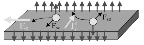
Figure 1: Schematics of the spin-Hall effect. An electric field applied along the $x$ axis, $E_{x}$, induces a transverse spin current $J^{z}_{y}$.

There are two extrinsic mechanisms of generation of transverse spin current: skew scattering and side jump Zhang (2000); Engel et al. (2005); Hankiewicz and Vignale (2006). They both arise from the effect of the spin-orbit interaction on electron-impurity collisions. Skew -scattering arises from the asymmetry of the electron-impurity scattering in the presence of spin-orbit interactions: electrons that are drifting in $+x$ direction under the action of electric field are more likely to be scattered to the left than to the right if, say their spin is up, while the reverse is true if their spin is down. This generates a net z-spin current in the y direction. This mechanism is also known as “Mott scattering” Mott and Massey (1964) and has been long known as a method to produce spin-polarized beams of particles.

The second effect is more subtle and is caused by the anomalous relationship between the physical and canonical position operator, as will be explained below. It is called “side-jump”, because semi-classically it can be derived from a lateral shift in the position of wave packet during collision with impurities. Without resorting to this description, we could arrive at the same side-jump term starting from the quantum kinetic equation and including the anomalous part of position operator. Figs. 2 and 3 present simple pictures of skew scattering and side jump mechanisms respectively.

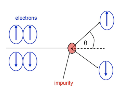
Figure 2: Schematic picture of the skew-scattering effect. Due to the spin-orbit interaction between electrons and impurities, electrons with different spin orientations are deflected to opposite edges of sample.

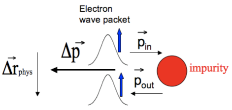
Figure 3: Schematic picture of the side-jump in a head-on collision with the impurity. The center of electron wave packet is shifted by $\Delta\vec{r}_{phys}$ in a direction perpendicular to the change of momentum during the collision. The physical origin of this shift is described in the text.

After this brief, pictorial presentation of different mechanisms contributing to the extrinsic spin-Hall effect, we are now ready to begin a more detailed analysis.

First of all, because both mechanisms depend crucially on the spin-orbit interaction, it is necessary to say something about the character of this interaction in the solid state. The derivation of this interaction involves steps that closely parallel the derivation of the spin-orbit interaction from the Dirac equation for a single electron in vacuum. In that case, we arrive at the effective one band (Pauli) Hamiltonian by applying a unitary transformationFoldy and Wouthuysen (1950) that decouples the electrons from the positrons, and then projecting onto the electron subspace. However, during this transformation the position operator is modified, taking the form

$$\vec{r}_{phys,i}=\vec{r}_{i}-\alpha_{0}(\vec{p}_{i}\times\vec{\sigma}_{i})~{},$$ (1)

where $\alpha_{0}\hbar=\hbar^{2}/4m_{e}^{2}c^{2}\approx-3.7\times 10^{-6}$Ų is the strength of spin-orbit interaction for bare electron in vacuum and $m_{e}$ is the bare electron mass. This physical position operator is valid for electrons in a conduction band. For a general case, one has to apply the form of $r_{phys}$ as shown in Eq. (74) of paper Sinitsyn (2008). Substitution of the modified position operator in the potential, followed by an expansion to first order in $\alpha_{0}$, leads to the standard form of the spin-orbit interaction in vacuum:

$$\hat{H}_{SO}=\alpha_{0}(\vec{p}\times\vec{\nabla}V(\vec{r}))\cdot\vec{\sigma}$$ (2)

where $V(\vec{r})$ is the external potential acting on an electron, $\vec{p}$ is the electron momentum and $\vec{\sigma}$ is the vector of the Pauli matrices. In semiconductors, the spin-orbit (SO) interactions play double role. First, we have SO effects induced by the periodic crystal potential $V_{0}(\vec{r})$. This causes splitting of the p-like valence band at $k=0$, in semiconductors like GaAs, into a fourfold degenerate band with total angular momentum $j=3/2$ (heavy and light hole bands) and “split-off band” with $j=1/2$. Further, the periodic crystal field gives rise to a small spin-orbit interaction of the order of $\frac{\hbar^{2}}{4m_{e}^{2}c^{2}}[\vec{p}\times\vec{\nabla}V_{0}(\vec{(}r))]\cdot\vec{\sigma}$ on electrons in the conduction band. Second, there is the SO interaction induced by any external potential (different than $V_{0}(\vec{r})$)if one wants to find an effective model say for the conduction band. In other words, if we perform a similar unitary transformation (as we did for the Dirac model) in a semiconductor, folding eight bands (conduction band, heavy and light hole bands as well as split-off valence band) into an effective model for the conduction band then the resulting spin-orbit interaction will be again of the same form as in Eq. (2), but with a much larger “coupling constant”: Winkler (2003)

$$\alpha=\frac{\hbar P^{2}}{3m_{e}^{2}}\left[\frac{1}{E_{g}^{2}}-\frac{1}{(E_{g}+\Delta_{SO})^{2}}\right]~{}$$ (3)

where $E_{g}$ is the gap energy between conduction and heavy/light holes bands, $\Delta_{SO}$ is the splitting energy between heavy/light holes and split-off bands, $P$ is the matrix element of the momentum operator between the conduction and the valence-band edges. Using values of the parameters appropriate for the 2DEG in Al_0.1Ga_0.9As Sih et al. (2005) with a conduction band mass $m=0.074m_{e}$ we find $\alpha\hbar=4.4\AA^{2}$. Therefore in the conduction band of semiconductors the spin-orbit interaction is six orders of magnitude larger than in vacuum and has the opposite sign. Obviously the spin-orbit interaction induced by the periodic crystal field on the conduction band can be omitted as a correction many orders of magnitude smaller. However, $\alpha\hbar$ is much smaller than the square of the effective Bohr radius in GaAs ( $10^{4}\AA^{2}$) and in this sense the spin-orbit coupling can still be considered a small perturbation. Notice that the form of the physical position operator for the conduction band is described by Eq. (1), with $\alpha_{0}$ replaced by $\alpha$.

Taking this into account and omitting for the time being the electron-electron interaction, we see that our effective Hamiltonian for electrons in the conduction band of GaAs takes the form

$$H_{ni}=H_{0}+V_{ei}(\vec{r}_{phys})+E(\vec{r}_{phys}),$$ (4)

where

$$H_{0}=\sum_{i}\frac{\vec{p_{i}}^{2}}{2m}$$ (5)

is the kinetic energy of electrons in conduction band ($m$ being the effective mass of the conduction band) and

$$V_{ei}(\vec{r}_{phys})\simeq V_{ei}(\vec{r}_{i})+\alpha\sum_{i}\left[\vec{p}_{i}\times\vec{\nabla}_{i}V_{ei}(\vec{r}_{i})\right]\cdot\vec{\sigma}_{i}$$ (6)

where $V_{ei}(\vec{r}_{i})$ is the impurity potential and the spin-orbit interaction between electrons and impurities arises from the Taylor expansion of the impurity potential around the canonical position operator $\vec{r}_{i}$. Finally,

$$E(\vec{r}_{phys})\simeq\sum_{i}\left\{e\vec{E}\cdot\vec{r}_{i}+e\alpha(\vec{p}_{i}\times\vec{E})\cdot\vec{\sigma}_{i}\right\}$$ (7)

where we took the interaction with the external electric field $\vec{E}$ to be $e\vec{E}\cdot\vec{r}_{phys}$.

The physical velocity operator is the time derivative of the physical position operator i.e.:

$$\vec{v}_{phys}=-\frac{i}{\hbar}[\vec{r}_{phys},\hat{H}],$$ (8)

and has the form

$$\vec{v}_{phys}=\frac{\vec{p}_{i}}{m}+\alpha\left[\vec{\nabla}_{i}V_{ei}({\vec{r}}_{i})+e\vec{E}\right]\times\vec{\sigma}_{i}-\alpha\frac{d\vec{p}_{i}}{dt}\times\sigma_{i},$$ (9)

where the first two terms on the right hand side are derivatives of the canonical position operator while the last term originates from the time derivative of the anomalous part of position operator. However, since the total force $\vec{F}_{i}=d\vec{p}_{i}/dt$ consists of a force originating from impurities and one from the electric field $F_{i}=-\vec{\nabla}_{i}V_{ei}({\vec{r}}_{i})-e\vec{E}$, the second and last terms of Eq. (9) are equivalent. Therefore $\vec{v}_{phys}$ can be written in the following compact form:

$$\vec{v}_{phys}=\frac{\vec{p}_{i}}{m}+2\alpha\left[\vec{\nabla}_{i}V_{ei}({\vec{r}}_{i})+e\vec{E}\right]\times\vec{\sigma}_{i}~{},$$ (10)

One can see that in our model the z-component of spin is conserved because it commutes with the Hamiltonian. We exploit the conservation of $\sigma_{z}$ by defining the quasi-classical one-particle distribution function $f_{\sigma}(\vec{r},\vec{k},t)$, i.e. the probability of finding an electron with $z$-component of the spin $S_{z}=\frac{\hbar}{2}\sigma$, with $\sigma=\pm 1$, at position $\vec{r}$ with momentum $\vec{p}=\hbar\vec{k}$ at the time $t$. In this review we focus on spatially homogeneous steady-state situations, in which $f_{\sigma}$ does not depend on $\vec{r}$ and $t$. We write

$$f_{\sigma}(\vec{r},\vec{k},t)=f_{0\sigma}(\epsilon_{k})+f_{1\sigma}(\vec{k})~{},$$ (11)

where $f_{0\sigma}(\epsilon_{k})$ is the equilibrium distribution function – a function of the free particle energy $\epsilon_{k}=\frac{\hbar^{2}k^{2}}{2m}$ – and $f_{1\sigma}(\vec{k})$ is a small deviation from equilibrium induced by the application of steady electric fields $\vec{E}_{\sigma}$ ($\sigma=\pm 1$) which couple independently to each of the two spin components. In the next few sections we will apply the Boltzmann equation approach to calculate $f_{1}$ taking spin Hall effect and spin Coulomb drag into account on equal footing.Hankiewicz and Vignale (2006)

To first order in $\vec{E}_{\sigma}$ the Boltzmann equation takes the form

$$-e\vec{E}_{\sigma}\cdot\frac{\hbar\vec{k}}{m}f^{\prime}_{0\sigma}(\epsilon_{k})=\dot{f}_{1\sigma}(\vec{k})_{c}~{},$$ (12)

where $f^{\prime}_{0\sigma}(\epsilon_{k})$ is the first derivative of equilibrium distribution function with respect to the energy and $\dot{f}_{1\sigma}(\vec{k})_{c}$ is the first-order in $\vec{E}_{\sigma}$ part of the collisional time derivative $\dot{f}_{\sigma}(\vec{k})_{c}$ due to various scattering mechanisms. For the electron-impurity scattering mechanism the collisional time derivative has the following form:

$$\dot{f}_{\sigma}(\vec{k})_{c,imp}=-\sum_{\vec{k}^{\prime}}\left[W_{\vec{k}\vec{k}^{\prime}\sigma}f_{\sigma}(\vec{k})-W_{\vec{k}^{\prime}\vec{k}\sigma}f_{\sigma}(\vec{k}^{\prime})\right]\delta(\widetilde{\epsilon}_{k\sigma}-\widetilde{\epsilon}_{k^{\prime}\sigma})$$

where $W_{\vec{k}\vec{k}^{\prime}\sigma}$ is the scattering rate for a spin-$\sigma$ electron to go from $\vec{k}$ to $\vec{k}^{\prime}$, and $\widetilde{\epsilon}_{k\sigma}$ is the particle energy, including an additional spin-orbit interaction energy due the electric field:

$$\widetilde{\epsilon}_{k\sigma}=\epsilon_{k}+2e\alpha\hbar\sigma(\vec{E}_{\sigma}\times\hat{z})\cdot\vec{k}~{},$$ (14)

The peculiar form of $\widetilde{\epsilon}_{k\sigma}$, which differs from the naive expectation $\epsilon_{k}+e\vec{E}\cdot\vec{r}_{phys}$ by a factor $2$ in the second term, is absolutely vital for a correct treatment of the “side-jump” contribution. The reason for the factor $2$ is that the $\delta$ function in Eq. (II) expresses the conservation of energy in a scattering process. Scattering is a time-dependent process: therefore the correct expression for the change in position of the electron $\Delta r_{phys}$ must be calculated as the integral of the velocity over time:

$$\Delta\vec{r}_{phys}=\int_{-\infty}^{\infty}\vec{v}_{phys}dt$$ (15)

Before solving integral in Eq. (15), let’s think for a moment about scattering event. Let’s take $\Delta\vec{p}=\vec{p}_{out}-\vec{p}_{in}$ (see Fig. (3)) to be the change in momentum of an electron wave packet during collision with an impurity. During the very short time of collision, $\nabla V(\vec{r})=-d\vec{p}/dt$ is very large and therefore second term of Eq. (10) completely dominates the velocity. Therefore, we disregard first term in the velocity formula and obtain a following form for the electron wave packet displacement:

$$\Delta\vec{r}_{phys}=-2\alpha\Delta\vec{p}\times\sigma/\hbar$$ (16)

Therefore, Eqs. (9,14,15) are consistent.

II.1 Skew-scattering

From the general scattering theory, developed for instance in Landau and Lifshitz (1964), one can deduce the form of scattering probability from $\vec{k}$ to $\vec{k}^{\prime}$ Kohn and Luttinger (1957); Hankiewicz and Vignale (2006) as:

$$W_{\vec{k}\vec{k}^{\prime},\sigma}=\left[W^{s}_{\vec{k}\vec{k}^{\prime}}+\sigma W^{a}_{\vec{k}\vec{k}^{\prime}}(\hat{k}\times\hat{k}^{\prime})_{z}\right]\delta(\epsilon_{k}-\epsilon_{k^{\prime}})~{},$$ (17)

where for centrally symmetric scattering potentials $W^{s}_{\vec{k}\vec{k}^{\prime}}$ and $W^{a}_{\vec{k}\vec{k}^{\prime}}$ depend on the magnitude of vectors $\vec{k}$ and $\vec{k}^{\prime}$ and the angle $\theta$ between them. Furthermore the left/right asymmetry of skew scattering is included explicitly in the factor $(\hat{k}\times\hat{k}^{\prime})_{z}$ and therefore both $W^{s}_{\vec{k}\vec{k}^{\prime}}$ and $W^{a}_{\vec{k}\vec{k}^{\prime}}$ are symmetric under interchange of $\vec{k}$ and $\vec{k^{\prime}}$. Taking into account the form of the scattering probability as well as the conservation energy during the scattering process we obtain following expression for the linearized collisional derivative:

$$\dot{f}_{1\sigma}(\vec{k})_{c,imp}=-\sum_{\vec{k}^{\prime}}W^{s}_{\vec{k}\vec{k}^{\prime}}\left\{f_{1\sigma}(\vec{k})-f_{1\sigma}(\vec{k}^{\prime})\right\}\delta(\epsilon_{k}-\epsilon_{k^{\prime}})$$

$$-\sigma\sum_{\vec{k}^{\prime}}W^{a}_{\vec{k}\vec{k}^{\prime}}(\hat{k}\times\hat{k}^{\prime})_{z}\left\{f_{1\sigma}(\vec{k})+f_{1\sigma}(\vec{k}^{\prime})\right\}\delta(\epsilon_{k}-\epsilon_{k^{\prime}})$$

$$+2\sigma\sum_{\vec{k}^{\prime}}W^{s}_{\vec{k}\vec{k}^{\prime}}f^{\prime}_{0\sigma}(\epsilon_{k})e\alpha\hbar(\vec{E}_{\sigma}\times\hat{z})\cdot(\vec{k}-\vec{k^{\prime}})\delta(\epsilon_{k}-\epsilon_{k^{\prime}})~{},$$

where $f_{1\sigma}(\vec{k})=-f^{\prime}_{0\sigma}(\epsilon_{k})\hbar\vec{k}\cdot\vec{V}_{\sigma}(k)$ and the first term on r.h.s. of this formula is the symmetric scattering term, the second one is the skew scattering term, while the last one will be ultimately responsible for the side jump. To find the drift velocity, $\vec{V}_{\sigma}(k)$, we need to multiply both sides of Boltzmann equation (12) by $\hbar\vec{k}/m$ and integrate over $\vec{k}$ space, and therefore derive $\vec{V}_{\sigma}(\vec{k})$ self-consistently from the condition:

$$-e\sum_{\vec{k}}\frac{\hbar\vec{k}}{m}\left[\vec{E}_{\sigma}\cdot\frac{\hbar\vec{k}}{m}\right]f^{\prime}_{0\sigma}(\epsilon_{k})=\sum_{\vec{k}}\frac{\hbar\vec{k}}{m}\dot{f}_{1\sigma}(\vec{k})_{c,imp}~{}.$$ (19)

After substituting of collisional derivative Eq. (II.1) into Eq. (19) and with the assumption that we can omit the k-dependence of drift velocity in low temperatures, we arrive at the following formula for $\vec{V}_{\sigma}$ to first order in the spin-orbit interaction:

$$\vec{V}_{\sigma}=\frac{-e\tau_{\sigma}}{m}\left[\vec{E}_{\sigma}-\sigma\frac{\tau_{\sigma}}{\tau_{\sigma}^{ss}}\vec{E}_{\sigma}\times\hat{z}\right]-2e\alpha\sigma(\vec{E_{\sigma}}\times\hat{z})~{},$$ (20)

where in the limit of zero temperature the symmetric scattering rate $1/\tau$ and the skew scattering rate $1/\tau_{ss}$ simplify to:

$$\frac{1}{\tau_{\sigma}}\stackrel{{\scriptstyle T\to 0}}{{\simeq}}\frac{m{\cal A}}{4\pi^{2}\hbar^{2}}\int_{0}^{2\pi}d\theta~{}W^{s}(k_{F},\theta)(1-\cos\theta)~{},$$ (21)

and

$$\frac{1}{\tau^{ss}_{\sigma}}\stackrel{{\scriptstyle T\to 0}}{{\simeq}}\frac{m{\cal A}}{4\pi^{2}\hbar^{2}}\int_{0}^{2\pi}d\theta~{}W^{a}(k_{F},\theta)\sin^{2}\theta~{}$$ (22)

.

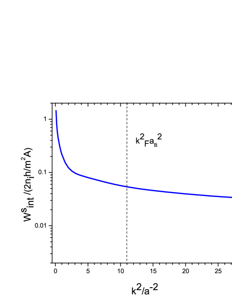
Figure 4: Integrated symmetric scattering rate in units of $2n_{i}h/m^{2}\cal A$ as a function of $k^{2}$ for a model circular well attractive potential $V_{0}=-5$meV and radius $a=9.45$nm (described in Reference Hankiewicz and Vignale (2006)). We choose the parameters typical for the experimental 2DEG confined in Al_0.1Ga_0.9As quantum well i.e. density of electrons and impurities $n_{2D}=n_{i}=2.0\times 10^{12}$cm^-2, $m=0.074$m_e, and mobility $\mu=0.1$m${}^{2}/$V.s. The effective spin-orbit coupling $\alpha\hbar=4.4{\AA}^{2}$ in accordance with Winkler (2003).

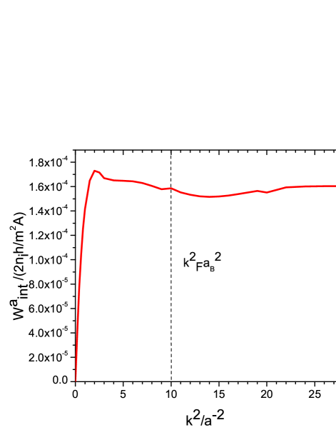
Figure 5: Integrated asymmetric scattering rate in units of $2n_{i}h/m^{2}\cal A$ as a function of $k^{2}$ for a model circular well attractive potential $V_{0}=-5$meV and radius $a=9.45$nm (described in Reference Hankiewicz et al. (2005)). We choose the parameters typical for the experimental 2DEG confined in Al_0.1Ga_0.9As quantum well i.e. density of electrons and impurities $n_{2D}=n_{i}=2.0\times 10^{12}$cm^-2, $m=0.074$m_e, and mobility $\mu=0.1$m${}^{2}/$V.s. The effective spin-orbit coupling $\alpha\hbar=4.4{\AA}^{2}$ in accordance with Winkler (2003).

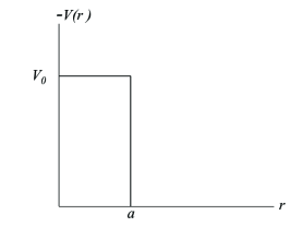
Figure 6: The electron-impurity potential V($\vec{r}$) used to estimate the ratio of symmetric to asymmetric scattering.

In Fig. (4) and Fig. (5), we present the integrated symmetric and asymmetric scattering rates calculated from Eqs. (21) and  (22) for a simple step potential of the form:

$$V(r)=V_{0}\theta(a-r)+\bar{\alpha}aL_{z}S_{z}\delta(r-a)V_{0}~{},$$ (23)

where $V_{0}$ is the attractive electron-impurity potential, $\bar{\alpha}=\alpha\hbar/a^{2}$ is the renormalized spin-orbit interaction, $\alpha$ is the effective spin-orbit coupling constant for the conduction band, $a$ is the impurity radius, $L_{z}$ and $S_{z}$ are the orbital angular and spin angular momenta, respectively. The simple step potential described in Eq. (23) is presented in Fig. (6). For parameters typical of III-V semiconductors, the asymmetric and symmetric scattering rates are almost flat as functions of the energy of the incoming electron (see Figs.  (4,5)). Comparing symmetric and asymmetric scattering rates one can find directly from picture, that for typical densities of 2DEG and typical Bohr radii in semiconductors the ratio of symmetric scattering time to skew scattering time is:

$$\frac{\tau}{\tau_{ss}}\approx 0.002\div 0.003$$ (24)

We assumed, in above discussion, that the electron-impurity potential is attractive, which is the most common case in semiconductors, where ionized donors play the role of impurities. However, the sign and the amplitude of skew scattering contribution (and more precisely skew scattering rate) depends strongly on the electron-impurity potential.

II.2 Side jump current and resistivity matrix

Now to determine the side jump contribution to the spin-Hall effect we need to carefully define the spin-current. The spin-current density operator must be calculated taking into account the form of the physical velocity (see Eq. (10)):

$$\hat{J}_{y}^{z} = -\frac{e}{2V}\sum_{i}\left(\upsilon^{y}_{phys,i}\sigma_{iz}+\sigma_{iz}\upsilon^{y}_{phys,i}\right)$$ (25)

$$= \frac{-e}{V}\sum_{i}\left(\frac{p^{y}_{i}\sigma_{iz}}{m}+\frac{2\alpha F_{ix}}{\hbar}\right)$$

$$\approx \frac{-e}{V}\sum_{i}\upsilon^{y}_{i}\sigma_{iz}$$

where the factor $2\alpha F_{ix}/\hbar$ vanishes because the net force $\vec{F}_{i}$ acting on an electron is zero when averaged over a steady-state ensemble. Therefore, the spin component of the current is

$$j_{\sigma} = -en_{\sigma}\vec{V_{\sigma}}\,,$$ (26)

and using Eq. (20) for the drift velocity we obtain the following form of side-jump current:

$$\vec{j}^{sj}=2e^{2}\alpha\sigma n_{\sigma}\vec{E}_{\sigma}\times z~{},$$ (27)

which evidently arises from the last term of Eq. (20). This simple form of the side-jump current is valid only for electrons in the conduction band. In this case, the side-jump current depends only on the spin-orbit coupling, the density of electrons and the spin-dependent electric field. The complete relation between the spin-component of current (from side jump and skew scattering contributions) and electric field has the following form:

$$\vec{E}_{\sigma}=\rho^{D}_{\sigma}\vec{j}_{\sigma}+\sigma[\rho^{ss}_{\sigma}-\lambda_{\sigma}\rho^{D}_{\sigma}]\vec{j}_{\sigma}\times\hat{z}$$ (28)

where $\rho^{D}_{\sigma}=\frac{m}{n_{\sigma}e^{2}\tau_{\sigma}}$ is the Drude resistivity, $\rho^{ss}_{\sigma}=\frac{m}{n_{\sigma}e^{2}\tau^{ss}_{\sigma}}$ is the skew scattering resistivity, and the last term in square brackets is the side-jump contribution to the resistivity: $\lambda_{\sigma}=\frac{2m\alpha}{\tau_{\sigma}}$. Eq. (28) yields to the following resistivity tensor (in the basis $x_{\uparrow}$, $y_{\uparrow}$, $x_{\downarrow}$, $y_{\downarrow}$):

$$\rho=\left(\begin{array}[]{llll}\rho^{D}_{\uparrow}&\rho^{ss}_{\uparrow}-\lambda_{\uparrow}\rho^{D}_{\uparrow}&0&0\\ -\rho^{ss}_{\uparrow}+\lambda_{\uparrow}\rho^{D}_{\uparrow}&\rho^{D}_{\uparrow}&0&0\\ 0&0&\rho^{D}_{\downarrow}&-\rho^{ss}_{\downarrow}+\lambda_{\downarrow}\rho^{D}_{\downarrow}\\ 0&0&\rho^{ss}_{\downarrow}-\lambda_{\downarrow}\rho^{D}_{\downarrow}&\rho^{D}_{\downarrow}\\ \end{array}\right)$$ (29)

The diagonal part of the resistivity reduces to the Drude formula $\rho_{\sigma}^{D}=\frac{m}{ne^{2}\tau_{\sigma}}$, as expected. The spin-orbit interaction is entirely responsible for the appearance of an off-diagonal (transverse) resistivity. The latter consists of two competing terms associated with side-jump ($\lambda_{\sigma}\rho^{D}_{\sigma}$) and skew-scattering ($\rho^{ss}_{\sigma}$), as seen in Eq. (29). The signs of side-jump and skew-scattering terms are opposite for attractive electron-impurity potential. Although, this is the most typical case in doped semiconductors, it is important to emphasize that side-jump and skew scattering terms have equal signs in the case of a repulsive electron-impurity potential. Also, as one can see from tensor  (29) contributions scale differently with the mobility. Since $\tau_{ss}\sim\tau$ the skew scattering contribution to the resistivity is proportional to $1/\mu$, where $\mu$ is a mobility, while the side jump contribution scales as $1/\mu^{2}$. The opposite signs of two contributions, and different scaling with mobility could allow to distinguish between them in the experiments (see Section IV) Hankiewicz et al. (2006). As expected, in the absence of electron-electron interactions, the resistivity tensor (29) does not include elements between the opposite spins.

III Spin-Coulomb drag

Ordinary Coulomb drag is caused by momentum exchange between electrons residing in two separate 2D layers and interacting via the Coulomb interaction (for review see Rojo (1999)). The Spin-Coulomb drag is the single-layer analogue of the ordinary Coulomb drag. In this case spin-up and spin-down electrons play the role of electrons in different layers and the friction arises (due to Coulomb interactions) when spin-up and spin-down electrons move within one single layer with different drift velocities D’Amico and Vignale (2000).

The simplest description of the spin-Coulomb drag is given in terms of a phenomenological friction coefficient $\gamma$. Later in the section we will show that the Boltzmann equation approach confirms this phenomenological description. Let us start with the equation of motion for the drift velocity of spin-$\sigma$ electrons:

$$m\dot{\vec{V}}_{\sigma}=-eN_{\sigma}\vec{E}_{\sigma}+\vec{F}_{\sigma,-\sigma}-\frac{m\vec{V}_{\sigma}}{\tau_{\sigma}}+\frac{m\vec{V}_{-\sigma}}{\tau^{\prime}_{\sigma}}$$ (30)

where $N_{\sigma}$ is the number of electrons with spin $\sigma$, $\vec{F}_{\sigma,-\sigma}$ is the net force exerted by $-\sigma$ spins on $\sigma$ spins, $\frac{1}{\tau_{\sigma}}$ is the rate of change of momentum of electrons with spin $\sigma$ due to electron-impurity scattering and is basically the Drude scattering rate, $\frac{\vec{V}_{-\sigma}}{\tau^{\prime}_{\sigma}}$ is the rate of change of momentum due to electron-impurity scattering in which electron flip its spin from $-\sigma$ to $\sigma$. From Newton’s third law one immediately sees:

$$\vec{F}_{\sigma,-\sigma}=-\vec{F}_{-\sigma,\sigma}$$ (31)

and by Galilean invariance this force can only depend on the relative velocity of the two components. Hence, for a weak Coulomb coupling one writes:

$$\vec{F}_{\sigma,-\sigma}=-\gamma N_{\sigma}(\vec{\upsilon}_{i,\sigma}-\vec{\upsilon}_{i,-\sigma})\frac{n_{-\sigma}}{n}$$ (32)

where $n_{\sigma}$ is the density of electrons with spin $\sigma$ and $\gamma$ is a spin-drag scattering rate. Taking into account Eq. (26) and applying Fourier transformation to Eq. (30) one gets following equation on the spin current density:

$$i\omega\vec{j}_{\sigma}(\omega) = \frac{-n_{\sigma}e^{2}\vec{E}_{\sigma}(\omega)}{m}+\left(\gamma\frac{n_{-\sigma}}{n}+\frac{1}{\tau_{\sigma}}\right)\vec{j}_{\sigma}(\omega)$$ (33)

$$- \left(\gamma\frac{n_{\sigma}}{n}+\frac{1}{\tau^{\prime}_{\sigma}}\right)\vec{j}_{-\sigma}(\omega)$$

Inverting Eq (33) gives us electric field:

$$\vec{E}_{\sigma}(\omega) = \left(\frac{-i\omega m}{n_{\sigma}e^{2}}+\frac{m}{n_{\sigma}e^{2}\tau_{\sigma}}+\frac{m\gamma}{ne^{2}}\frac{n_{-\sigma}}{n_{\sigma}}\right)\vec{j}_{\sigma}(\omega)$$ (34)

$$- \left(\frac{m}{n_{\sigma}e^{2}\tau^{\prime}_{\sigma}}+\frac{m\gamma}{ne^{2}}\right)\vec{j}_{-\sigma}(\omega)$$

From this we can immediately read the resistivity tensor. Its real part, in the basis of $x_{\uparrow}$, $x_{\downarrow}$, has following form:

$$\rho=\left(\begin{array}[]{cc}\rho^{D}_{\uparrow}+\rho^{SD}n_{\downarrow}/n_{\uparrow}&-\rho^{SD}-\rho^{\prime}_{\uparrow}\\ -\rho^{SD}-\rho^{\prime}_{\downarrow}&\rho^{D}_{\downarrow}+\rho^{SD}n_{\uparrow}/n_{\downarrow}\\ \end{array}\right)$$ (35)

where $\rho^{SD}=m\gamma/ne^{2}$ is the spin Coulomb drag resistivity and $\rho^{\prime}_{\sigma}=m/n_{\sigma}e^{2}\tau^{\prime}_{\sigma}$. Several features of this matrix are noteworthy. First the matrix is symmetric. Second the off-diagonal terms are negative. The minus sign can be easily explained. $\rho_{\uparrow\downarrow}$ is the electric field induced in the up-spin channel by a current flowing in the down-spin channel when the up spin current is zero. Since a down spin current in the positive direction tends to drag along the up-spins, a negative electric field is needed to maintain the zero value of the up-spin current. There is no limit on the magnitude of $\rho_{SD}$. The only restriction is that the eigenvalues of the real part of the resistivity matrix should be positive to ensure positivity of dissipation. Finally, the spin-Coulomb drag appears in both diagonal and off-diagonal terms so the total contribution cancels to zero (in accordance with Eq. (31)) if the drift velocities of up and down spins are equal.

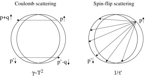
Figure 7: Comparison of Coulomb scattering with the spin-flip scattering. At finite temperature Coulomb scattering can be a more effective mechanism of momentum exchange between up- and down-spin populations than spin-flip collisions with impurities.

Let us take a closer look at the competing off-diagonal terms: spin-Coulomb drag and spin-flip resistivities. At very low temperature spin flip processes win because in this limit the Coulomb scattering is suppressed by phase space restrictions (Pauli’s exclusion principle) and $\gamma$ tends to zero as $T^{2}$ in three dimensions and $T^{2}lnT$ in 2D. However, the spin-flip processes from electron-impurity collisions do not effectively contribute to momentum transfer between two spin-channels. An up-spin electron that collides with an impurity and flips its spin orientation from up to down is almost equally likely to emerge in any direction, as shown in Fig. (7), so the momentum transfer from the up to the down spin orientation is minimal and independent of what the down spins are doing. However, the situation looks quite different for electron-electron collisions: the collision of an up-spin electron with a down-spin electron leads to a momentum transfer that is preferentially oriented against the relative velocity of the two electrons (see Fig. (7)) and is proportional to the latter. Taking the spin-flip relaxation time to be of the order of 500ns (ten times larger than spin-relaxation time in GaAs Kikkawa et al. (1997); Kikkawa and Awschalom (1998)), and the value of $\frac{1}{\gamma}$ of the order of the Drude scattering time, around 1 ps D’Amico and Vignale (2002, 2003), and temperatures of the order of the Fermi energy $T_{F}\sim 300K$ we estimate that the spin-Coulomb drag contribution will dominate already for $T\sim 0.3K$. Further, for mobilities typical for semiconductors 10⁴ $\div$ 10⁵ cm²/Vs the ratio of spin-Coulomb drag to the Drude resistivity can be as large as ten (see more detailed discussion in the next Section and Fig. (9)).

Returning to Boltzmann approach, the electron-electron contribution to the collisional derivative has the formD’Amico and Vignale (2002)

$$\dot{f}_{\sigma}(\vec{k})_{c,e-e}\simeq-\sum_{\vec{k}^{\prime}\vec{p}\vec{p}^{\prime}}W_{C}(\vec{k}\sigma,\vec{p}-\sigma;\vec{k}^{\prime}\sigma,\vec{p}^{\prime}-\sigma)\left\{f_{\sigma}(\vec{k})f_{-\sigma}(\vec{p})[1-f_{\sigma}(\vec{k}^{\prime})][1-f_{-\sigma}(\vec{p}^{\prime})]\right.$$

$$\left.-f_{\sigma}(\vec{k}^{\prime})f_{-\sigma}(\vec{p}^{\prime})[1-f_{\sigma}(\vec{k})][1-f_{-\sigma}(\vec{p})]\right\}\delta_{\vec{k}+\vec{p},\vec{k}^{\prime}+\vec{p}^{\prime}}\delta(\widetilde{\epsilon}_{k\sigma}+\widetilde{\epsilon}_{p-\sigma}-\widetilde{\epsilon}_{k^{\prime}\sigma}-\widetilde{\epsilon}_{p^{\prime}-\sigma})~{},$$ (36)

where $W_{C}(\vec{k}\sigma,\vec{p}-\sigma;\vec{k}^{\prime}\sigma,\vec{p}^{\prime}-\sigma)$ is the electron-electron scattering rate from $\vec{k}\sigma,\vec{p}-\sigma$ to $\vec{k}^{\prime}\sigma,\vec{p}^{\prime}-\sigma$, and the Pauli factors $f_{\sigma}(\vec{k})$, $1-f_{\sigma}(\vec{k}^{\prime})$ etc. ensure that the initial states are occupied and the final states empty as required by Pauli’s exclusion principle. Notice that, for our purposes, only collisions between electrons of opposite spins are relevant, since collision between same-spin electrons conserve the total momentum of each spin component. After substituting the linearized Boltzmann equation into Eq. (III) and in the absence of spin-orbit interactions one derives the following Coulomb collision integral Hankiewicz et al. (2005):

$$\dot{f}_{\sigma}(\vec{k})_{c,e-e}\simeq-\frac{1}{k_{B}T}\sum_{\vec{k}^{\prime}\vec{p}\vec{p}^{\prime}}W_{C}(\vec{k}\sigma,\vec{p}-\sigma;\vec{k}^{\prime}\sigma,\vec{p}^{\prime}-\sigma)[\hbar\vec{V}_{\sigma}-\hbar\vec{V}_{-\sigma}](\vec{k}-\vec{k}^{\prime})$$ (37)

$$f_{0\sigma}(\epsilon_{k})f_{0-\sigma}(\epsilon_{p})f_{0\sigma}(-\epsilon_{k^{\prime}})f_{0-\sigma}(-\epsilon_{p^{\prime}})\delta_{\vec{k}+\vec{p},\vec{k}^{\prime}+\vec{p}^{\prime}}\delta(\epsilon_{k\sigma}+\epsilon_{p-\sigma}-\epsilon_{k^{\prime}\sigma}-\epsilon_{p^{\prime}-\sigma})~{},$$

where $T$ is the temperature, $k_{B}$ is the Boltzmann constant, and we have made use of the identity $f_{0\sigma}(\epsilon_{k})f_{0-\sigma}(\epsilon_{p})[1-f_{0\sigma}(\epsilon_{k^{\prime}})][1-f_{0-\sigma}(\epsilon_{p^{\prime}})]=[1-f_{0\sigma}(\epsilon_{k})][1-f_{0-\sigma}(\epsilon_{p})]f_{0\sigma}(\epsilon_{k^{\prime}})f_{0-\sigma}(\epsilon_{p^{\prime}})$ for $\epsilon_{k\sigma}+\epsilon_{p-\sigma}-\epsilon_{k^{\prime}\sigma}-\epsilon_{p^{\prime}-\sigma}=0$. The collision integral Eq (37) is proportional to the difference of velocities for spin-up and spin-down electrons. Therefore if a finite spin current is set up through the application of an external field, then the Coulomb interaction will tend to equalize the net momenta of the two spin components, causing $\langle V_{\uparrow}\rangle$ -$\langle V_{\downarrow}\rangle$ to decay and thus can be interpreted, as we explained before, as a damping mechanism for spin-current.

After substituting Eq. (37) into self-consistent equation for a drift velocity Eq. (19), one obtains the spin-drag coefficient $\gamma$ i.e. the rate of momentum transfer between up and down spin electrons:

$$\gamma = \frac{n}{n_{\sigma}n_{-\sigma}}\sum_{\vec{k}\vec{k}^{\prime}\vec{p}\vec{p}^{\prime}}W_{C}(\vec{k}\sigma,\vec{p}-\sigma;\vec{k}^{\prime}\sigma,\vec{p}^{\prime}-\sigma)$$ (38)

$$\frac{(\vec{k}-\vec{k}^{\prime})^{2}}{4mk_{B}T}f_{0\sigma}(\epsilon_{k})f_{0-\sigma}(\epsilon_{p})f_{0\sigma}(-\epsilon_{k^{\prime}})f_{0-\sigma}(-\epsilon_{p^{\prime}})$$

$$\times \delta_{\vec{k}+\vec{p},\vec{k}^{\prime}+\vec{p}^{\prime}}\delta(\epsilon_{k\sigma}+\epsilon_{p-\sigma}-\epsilon_{k^{\prime}\sigma}-\epsilon_{p^{\prime}-\sigma}).$$

as well as equation of motion Eq. (30) and resistivity tensor Eq. (43) derived before through phenomenological approach.

Let us now describe briefly the idea of spin-grating experiments Weber et al. (2005), where the spin-Coulomb drag has been observed. A periodic spin density can be induced by letting two linearly polarized light beams coming from different directions interfere on the surface of a two-dimensional electron gas. This interference produces a spatially varying pattern of polarization, with alternating regions of left-handed and right-handed circular polarization separated by linearly polarized regions. The spin density is optically induced in the regions of circular polarization. More precisely, the regions of right-handed circular polarization have a larger up-spin density while the regions of left-handed circular polarization have a larger down-spin density. At a given time $t=0$ the pump light is turned off and the subsequent time evolution of the spin-density is monitored by Kerr spectroscopy. In Kerr spectroscopy, one measures the amplitude of the spin-density modulation by looking at the rotation of the plane of polarization of the light diffracted by the spin-grating. The initial rate of decay of the spin grating amplitude $\gamma_{q}$ depends on the wave vector q of the grating in the following manner:Weber et al. (2005)

$$\gamma_{q}=\frac{1}{\tau_{s}}+D_{s}q^{2}$$ (39)

where $\tau_{s}$ is the spin density relaxation time and $D_{s}$ is the spin diffusion constant. Therefore $D_{s}$ can be found from the slope of $\gamma_{q}$ vs. $q^{2}$. The spin diffusion constant in the presence of spin-Coulomb drag was discussed in detail in D’Amico and Vignale (2001); Vignale (2007) and has the following form:

$$\frac{D_{s}}{D^{0}_{s}}=\frac{\chi_{s}^{0}/\chi_{s}}{1+\gamma\tau}$$ (40)

where $D^{0}_{s}$ is the spin diffusion constant for the non-interacting system, $\chi_{s}^{0}$ is the spin-susceptibility for non-interacting system and $\chi_{s}$ is the interacting spin-susceptibility, with Landau-Fermi-liquid corrections taken into account.

Actually, from the analysis presented in Refs. D’Amico and Vignale (2001); Vignale (2007) one expects that the experimentally determined $D_{s}$ should include two effects: the Fermi liquid correction to the spin susceptibility Giuliani and Vignale (2005) and the spin-Coulomb drag correction. However, the Fermi liquid correction to the spin susceptibility is quite small. It is given by the well-known formula Giuliani and Vignale (2005)

$$\frac{\chi^{0}_{S}}{\chi_{S}}=\frac{1+F_{0}^{a}}{\frac{m}{m_{e}}}$$ (41)

where $m/m_{e}$ is the many-body mass enhancement and $F_{0}^{a}$ is the Landau parameter described in detail in Ref. Giuliani and Vignale (2005). Since the $m/m_{e}\sim 0.96$ and $F_{0}^{a}\sim-0.2$, the interacting spin susceptibility will be enhanced by no more than 20-30% and obviously will be independent of mobility of 2DEG. Therefore, the Fermi liquid corrections to the spin-conductivity are very small in comparison with the spin-Coulomb drag corrections and the spin-Coulomb drag will be the main effect influencing the spin transport. Indeed, the experimentally determined $D_{s}$ Weber et al. (2005) was found to be in excellent agreement with the theoretically predicted values for a strictly two-dimensional electron gas in the random phase approximation D’Amico and Vignale (2001, 2003). Following this, Badalyan et al. Badalyan et al. (2008) noticed that the inclusion of the finite thickness of the two-dimensional electron gas in the GaAs quantum well would worsen the agreement between theory and experiment, because the form factor associated with the finite thickness of the quantum well reduces the effective electron-electron interaction at momentum transfers of the order of the Fermi momentum, which are the most relevant for spin Coulomb drag. Fortunately, it turned out that this reduction is compensated by the inclusion of many-body effects beyond the random phase approximation, namely local-field effects which, to a certain extent, strengthen the effective Coulomb interaction by reducing the electrostatic screening.Badalyan et al. (2008) The final upshot of the more careful analysis is that the theory remains in quantitative agreement with experiment in a broad range of temperatures.

IV Influence of spin-Coulomb drag on the extrinsic spin-Hall effect.

IV.1 Resistance tensor

In this Section we study the influence of electron-electron interactions on the spin-Hall effect. Main discussion concerns 2DEG, however at the end of this Section we will comment on the behavior of spin-Hall conductivity in bulk materials. We start from the Hamiltonian which includes electron-electron interactions:

$$\hat{H}=\hat{H}_{ni}+\frac{1}{2}\sum_{i\neq j}\frac{e^{2}}{\epsilon_{b}|\vec{r}_{i}-\vec{r}_{j}|}+\alpha\sum_{i}\vec{p}_{i}\times\vec{\nabla}_{i}V^{i}_{ee}\cdot\vec{\sigma}_{i}$$ (42)

where $\hat{H}_{ni}$ is defined by Eq. (4) and $V_{ee}=\sum_{i\neq j}\frac{e^{2}}{\epsilon_{b}|\vec{r}_{i}-\vec{r}_{j}|}$. Notice that the electric potential coming from electron-electron interactions, like every potential whose gradient is non-zero, generates the spin-orbit term in Hamiltonian. This new spin-orbit term, introduces a new contribution to the Coulomb collision integral: $2e\alpha\hbar\sigma(\vec{E}_{\sigma}+\vec{E}_{-\sigma})\times\hat{z}(\vec{k}-\vec{k}^{\prime})$ which adds up to previous term i.e. the difference of velocities for spin-up and down (see Eq. (37)). As a consequence, electron traveling say in x direction with spin up can be scattered in a y direction with simultaneous spin-flip, i.e. resistivity tensor contains terms which connect y and x components with opposite spins. The full resistivity matrix in the basis of $x_{\uparrow}$, $y_{\uparrow}$, $x_{\downarrow}$, $y_{\downarrow}$ has the following form:

$$\rho=\left(\begin{array}[]{llll}\rho^{D}_{\uparrow}+\rho^{SD}n_{\downarrow}/n_{\uparrow}&\rho^{ss}_{\uparrow}-\lambda_{\uparrow}\rho^{D}_{\uparrow}+A^{\gamma\alpha}_{\uparrow}&-\rho^{SD}-\rho^{\prime}_{\uparrow}&B^{\gamma\alpha}_{\uparrow}\\ -\rho^{ss}_{\uparrow}+\lambda_{\uparrow}\rho^{D}_{\uparrow}-A^{\gamma\alpha}_{\uparrow}&\rho^{D}_{\uparrow}+\rho^{SD}n_{\downarrow}/n_{\uparrow}&-B^{\gamma\alpha}_{\uparrow}&-\rho^{SD}-\rho^{\prime}_{\uparrow}\\ -\rho^{SD}-\rho^{\prime}_{\downarrow}&-B^{\gamma\alpha}_{\downarrow}&\rho^{D}_{\downarrow}+\rho^{SD}n_{\uparrow}/n_{\downarrow}&-\rho^{ss}_{\downarrow}+\lambda_{\downarrow}\rho^{D}_{\downarrow}-A^{\gamma\alpha}_{\downarrow}\\ B^{\gamma\alpha}_{\downarrow}&-\rho^{SD}-\rho^{\prime}_{\downarrow}&\rho^{ss}_{\downarrow}-\lambda_{\downarrow}\rho^{D}_{\downarrow}+A^{\gamma\alpha}_{\downarrow}&\rho^{D}_{\downarrow}+\rho^{SD}n_{\uparrow}/n_{\downarrow}\\ \end{array}\right)$$ (43)

where $\rho^{SD}=m\gamma/ne^{2}$ is the spin Coulomb drag resistivity and $\rho^{\prime}_{\sigma}=m/n_{\sigma}e^{2}\tau^{\prime}_{\sigma}$ (recall that $\lambda_{\sigma}=\frac{2m\alpha}{\tau_{\sigma}}$ is a dimensionless quantity). $A^{\gamma\alpha}_{\sigma}$ and $B^{\gamma\alpha}_{\sigma}$ represent the terms of the first order in electron-electron coupling $\gamma$ and in SO coupling $\alpha$ and are defined as follows: $A^{\gamma\alpha}_{\sigma}=-\lambda_{\sigma}\rho_{SD}n_{-\sigma}/n_{\sigma}+2m\alpha\gamma[-n_{-\sigma}\rho^{D}_{\sigma}/n+(n_{-\sigma}/n-n^{2}_{-\sigma}/nn_{\sigma})\rho^{SD}]$ and $B^{\gamma\alpha}_{\sigma}=\lambda_{\sigma}\rho_{SD}+2m\alpha\gamma[-n_{-\sigma}\rho^{D}_{-\sigma}/n+(n_{-\sigma}/n-n_{\sigma}/n)\rho^{SD}]$. Notice that the resistivity satisfies the following symmetry relations:

$$\rho^{\beta\beta^{\prime}}_{\sigma\sigma}=-\rho^{\beta^{\prime}\beta}_{\sigma\sigma}$$ (44)

$$\rho^{\beta\beta^{\prime}}_{\sigma-{\sigma}}=\rho^{\beta^{\prime}\beta}_{-{\sigma}\sigma}$$ (45)

where upper indices $\beta$ and $\beta^{\prime}$ denote directions, and the lower ones spin orientations. New features of the resistivity matrix 43 are the $\gamma\alpha$ and $\gamma^{2}\alpha$ terms, which appear in the transverse elements of the resistivity when the system is spin-polarized. Furthermore, the off-diagonal resistivity elements $\rho_{xy}^{\sigma-\sigma}$ are generally non zero. In the paramagnetic case (zero spin polarization) the $\alpha\gamma^{2}$ terms are zero and the resistivity matrix simplifies significantly. In this case, we find simple interrelations between currents and electric fields in the spin and charge channels. Omitting spin-flip processes ($1/\tau^{\prime}=0$) we obtain

$$\vec{E}_{c}=\rho^{D}\vec{j}_{c}+2(\rho^{ss}-\lambda\rho^{D}-\lambda\rho_{SD})\vec{j}_{s}\times\hat{z}~{},$$ (46)

$$\vec{E}_{s}=4(\rho^{SD}+\rho^{D})\vec{j}_{s}+2(\rho^{ss}-\lambda\rho^{D}-\lambda\rho_{SD})\vec{j}_{c}\times\hat{z}~{},$$ (47)

where the charge/spin components of the electric field are defined as $\vec{E}_{c}=\frac{\vec{E}_{\uparrow}+\vec{E}_{\downarrow}}{2}$, $\vec{E}_{s}=\vec{E}_{\uparrow}-\vec{E}_{\downarrow}$, and the charge and spin currents are $\vec{j}_{c}=\vec{j}_{\uparrow}+\vec{j}_{\downarrow}$ and $\vec{j}_{s}=\frac{\vec{j}_{\uparrow}-\vec{j}_{\downarrow}}{2}$, respectively. The spin-Coulomb drag renormalizes the longitudinal resistivity only in the spin channel. This is a consequence of the fact that the net force exerted by spin-up electrons on spin-down electrons is proportional to the difference of their drift velocities, i.e. to the spin current. Additionally, the electron-electron corrections to the spin-orbit interactions renormalize the transverse resistivity in the charge and spin channels, so the Onsager relations between spin and charge channels hold.

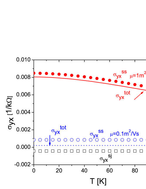
Figure 8: Spin Hall conductivity as a function of temperature at constant mobility. $\sigma_{yx}^{sj}$(open black squares), $\sigma_{yx}^{ss}$ (open blue and close red circles),$\sigma_{yx}^{tot}$ (red solid line and dashed blue line) are the side-jump, skew-scattering and the total spin conductivity in a presence of electron-electron interactions. Notice that only skew scattering conductivity is modified by spin-Coulomb drag. Red and blue curves/symbols are for $\mu=1$m${}^{2}/$V.s, and $\mu=0.1$m${}^{2}/$V.s. We choose the parameters typical for the experimental 2DEG confined in Al_0.1Ga_0.9As quantum well i.e. density of electrons and impurities $n_{2D}=n_{i}=2.0\times 10^{12}$cm^-2, $m=0.074$m_e, and two sets of mobilities and relaxation times: $\mu=0.1$m${}^{2}/$V.s, $\tau=4\times 10^{-5}$ns $\tau_{ss}=0.02$ns and $\mu=1$m${}^{2}/$V.s $\tau=4\times 10^{-4}$ns $\tau_{ss}=0.2$ns. The effective spin-orbit coupling $\alpha\hbar=4.4{\AA}^{2}$ in accordance with Winkler (2003). We used the model potential (see appendix) where an effective impurity radius $a=9.45$nm, the height of attractive impurity potential $V_{0}=-5$meV for $\mu=0.1$m${}^{2}/$V.s and $V_{0}=-1.6$meV for $\mu=1$m${}^{2}/$V.s.

Under the assumption that the electric field is in the $x$ direction and has the same value for spin up and spin down electrons we see that Eq. (46) and Eq. (47) yield the following formula for the spin current $j^{z}_{s,y}=j_{\uparrow}-j_{\downarrow}$ in $y$ direction:

$$j^{z}_{s,y}=\left[\frac{\rho^{ss}/(\rho^{D})^{2}}{1+\rho^{SD}/\rho^{D}}-\frac{\lambda}{\rho_{D}}\right]E_{x}$$ (48)

The first term in the square brackets is associated with the skew-scattering, while the second is the side-jump contribution. Notice that the side-jump conductivity $\sigma^{sj}=-\frac{\lambda}{\rho_{D}}=-2\alpha ne^{2}$ depends neither on the strength of disorder nor on the strength of the electron-electron interaction. Moreover, as we showed in Hankiewicz et al. (2006) by using a gauge invariance condition, the side jump does not depend on the electron-impurity and electron-electron scattering potential to all orders in both these interactions. By contrast, the skew scattering contribution to the spin conductivity, in the absence of e-e interactions scales with transport scattering time. Therefore for very clean samples, the skew scattering contribution would tend to infinity. However, this unphysical behavior is cured by the presence of spin-Coulomb drag, which sets an upper limit to the spin conductivity of the electron gas: so the skew scattering term scales as $\tau/(1+\rho_{SD}/\rho_{D})=\tau/(1+\gamma\tau)$, which tends to a finite limit for $\tau\to\infty$. Let us now make an estimate of skew scattering contribution to the spin-Hall condutivity. Using the typical ratio of $\tau/\tau_{ss}\approx 10^{-3}$ (see Eq. (24) we obtains:

$$\sigma^{ss}=10^{-3}\frac{\sigma_{D}}{1+\gamma\tau}$$ (49)

We will use this estimate in Section VI to compare importance of different contributions to the spin-Hall conductivity.

Also, the direct dependence of the skew scattering conductivity (see Eq. (49)) on the transport scattering time $\tau$ is the reason why this term is modified by spin-Coulomb drag. By contrast, the side-jump conductivity, which is independent of $\tau$, remains completely unaffected. The total spin Hall conductivity may either decrease or increase as a result of the spin Coulomb drag, depending on the relative sign and size of the skew-scattering and side-jump contributions. In the ordinary case of attractive impurities, when the skew-scattering contribution dominates, we expect an overall reduction in the absolute value of the spin Hall conductivity.

This is shown in Fig. (8). One can see that in high-mobility samples the spin Coulomb drag reduces the spin-Hall conductivity very effectively. There is no upper limit to the reduction of the spin-Hall conductivity since the factor $1+\gamma\tau$ can become arbitrarily large with increasing mobility. The behavior of $\gamma\tau$ as a function of temperature is shown in Fig. (9) for a typical semiconductor mobility, $\mu=3\times 10^{4}$ cm²/V.s. For example, in a two-dimensional GaAs quantum well at a density $n=10^{11}$ cm^-2 and mobility $3\times 10^{4}$ cm²/V.s the factor $\gamma\tau$ is quite significantly larger than one in a wide range of temperatures from $50$ K up to room temperature and above, and can substantially reduce the skew scattering term.

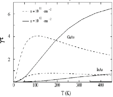
Figure 9: The ratio of spin-Coulomb drag to Drude resistance $\gamma\tau$ as a function of temperature for GaAs and InAs 2DEG with mobility $\mu=3\times 10^{4}$ cm²/V.s. The dashed and solid lines correspond to $n=10^{11}cm^{-2}$ and $n=10^{12}cm^{-2}$, respectively.

Let us finally comment on the spin-Hall conductivity in 3D. Although the general formulas are the same as in 2D, the actual value of $\rho^{ss}$ must be obtained by solving a three-dimensional scattering problem. This has been done in Ref. Engel et al. (2005) for the following model attractive potential between the electron and an impurity atom:

$$V(r)=\frac{-e^{-q_{s}r}e^{2}}{\epsilon r}$$ (50)

where $\epsilon$ is permittivity of material and $1/q_{s}$ is the screening length associated with the Thomas-Fermi screening. For this model potential, the spin-Hall conductivity takes the form:

$$\sigma^{SH}=-2\alpha ne^{2}+\frac{\gamma_{s}}{2}\sigma_{D}$$ (51)

where $\sigma_{D}$ is the Drude conductivity and $\gamma_{s}$ is a skewdness parameter, given approximately by $\gamma_{s}=4\alpha\hbar/(a_{B}^{2})$.Engel et al. (2005) Notice that the side-jump contribution has exactly the same form as in 2D. Further, in 3D the spin-Coulomb drag should modify the spin-Hall conductivity in a similar way i.e. by renormalizing the skew-scattering by factor 1+$\gamma\tau$ while leaving the side jump contribution to the spin-conductivity unchanged. Therefore except for the different scaling of $\gamma$ with temperature the spin-Hall conductivity behaves very similarly in 2D and in 3D.D’Amico and Vignale (2002, 2003)

IV.2 Spin accumulation

A quantitative theory of the spin accumulation in semiconductors requires in general a proper treatment of the boundary conditions as well as electron-hole recombination effects Tse et al. (2005). In this chapter we will study the influence of spin-Coulomb drag on spin accumulation assuming that electrons are the only carriers involved in transport. Our goal is to interpret the optical experiments in which spin accumulation is measured (Sih et al. (2005); Kato et al. (2004)). Notice that in previous theoretical papers Engel et al. (2005); Hankiewicz and Vignale (2006), directions of electric field and spin accumulation where exchanged in relation to experimental ones which led to a difference in a sign between experiment and theoretical predictions due to the following relation between resistivities: $\rho^{SH}_{xy}=-\rho^{SH}_{yx}$. In this review we finally clarify this point and show that the sign of experimental and theoretical spin-accumulations agree.

We consider a very long conductor in the form of a bar of length $L$ in the $y$ direction and narrow width $W$ in the $x$ direction, exactly the same setup as in experiments Sih et al. (2005); Kato et al. (2004) (see Fig (10b)). A charge current flows only in the $y$ direction. The spin components of the transverse current $j_{\sigma}^{x}$, with $\sigma=\uparrow$ or $\downarrow$ add up to zero everywhere and individually vanish on the edges of the system, i.e. $j_{\sigma}^{x}=0$ at $x=\pm W/2$. In order to satisfy the boundary conditions the system cannot remain homogeneous in the $x$-direction. A position-dependent spin density, known as spin accumulation develops across the bar, and is reflected in non-uniform chemical potentials $\mu_{\sigma}(x)$. In the steady state regime the spatial derivative of the spin-current in the $x$-direction must exactly balance the relaxation of the spin density due to spin-flip processes i.e.:

$$\frac{e}{\sigma_{s}}\frac{dJ_{s}}{dx}=\frac{\mu_{\sigma}(x)-\mu_{-\sigma}(x)}{L_{s}^{2}}$$ (52)

where $L_{s}$ is the spin diffusion length and $\sigma_{s}$ is the longitudinal spin-conductivity. Additionally, Ohm’s law must be fulfilled:

$$J_{s}=\sigma_{s}(E^{x}_{\sigma}-E^{x}_{-\sigma})$$ (53)

where the effective electric field in the $x$- direction is equivalent to the gradient of chemical potential:

$$eE^{x}_{\sigma}=d\mu_{\sigma}/dx~{}.$$ (54)

Notice that in the limit of infinite spin-relaxation time ($L_{s}\to\infty$) the divergence of spin-current equals zero and the spin accumulation can be obtained directly from the homogeneous formulas, Eqs. (46) and (47). In an inhomogenous case, combined Eq. (52) and Eq. (53) lead to the following equation for the spin accumulations Valet and Fert (1993)

$$\frac{d^{2}[\mu_{\sigma}(x)-\mu_{-\sigma}(x)]}{d^{2}x}=\frac{\mu_{\sigma}(x)-\mu_{-{\sigma}}(x)}{L_{s}^{2}}~{},$$ (55)

whose solution is:

$$\mu_{\sigma}(x)-\mu_{-{\sigma}}(x)=Ce^{\frac{x}{L_{s}}}+C^{\prime}e^{-\frac{x}{L_{s}}}~{},$$ (56)

and C, C’ are constants to be determined by the boundary conditions $j^{x}_{\pm\sigma}(\pm W/2)=0$. Additionally using Eq. (54) and the resistivity tensor we can write the boundary conditions for $E^{x}_{\sigma}(\pm W/2)$. Using the boundary conditions for the spin-dependent chemical potentials and the spin-dependent electric fields one finally finds the following formula for the spin accumulation in a paramagnetic case:

$$\mu_{\uparrow}(x)-\mu_{\downarrow}(x)=\frac{2eL_{s}E_{y}[\rho^{ss}-\lambda\rho^{D}-\lambda\rho_{SD}]\sinh(x/L_{s})}{\rho_{D}\cosh(W/2L_{s})}~{}$$

. (57)

The formula for the spin-accumulation in a spin-polarized case can be also easily obtained and the interested reader can find it in Ref.Hankiewicz and Vignale (2006). Finally, the spin-accumulation at the edges of sample for $L=W/2$ has the form:

$$V_{ac}^{x}=\mu_{\uparrow}(W/2L_{s})-\mu_{\downarrow}(W/2L_{s})=$$

$$2eL_{s}j_{y}[\rho^{ss}-\lambda\rho^{D}-\lambda\rho_{SD}]\tanh(W/2L_{s})~{}.$$ (58)

The three terms in the square brackets of Eq. (IV.2) are the skew-scattering term, the ordinary side-jump contribution, and a Coulomb correction which has its origin in the side-jump effect. The latter is not a spin Coulomb drag correction in the proper sense, for in this case the transverse spin current, and hence the relative drift velocity of the electrons, is zero. What happens here is that the spin Hall current is canceled by an oppositely directed spin current, which is driven by the gradient of the spin chemical potential. Now the spin Hall current contains a universal contribution, the side-jump term, which is not affected by Coulomb interaction, but at the same time the constant of proportionality between the spin current and the gradient of the spin chemical potential, that is to say the longitudinal spin conductivity, is reduced by the Coulomb interaction. Therefore, in order to maintain the balance against the unchanging side-jump current, the absolute value of the gradient of the spin chemical potential must increase when the Coulomb interaction is taken into account. This effect may increase or decrease the total spin accumulation, depending on the relative sign and magnitude of the side-jump and skew scattering contributions. It reduces it in the common case, for an attractive electron-impurity potential, where the two contributions have opposite signs and the skew-scattering dominates.

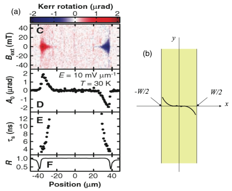
Figure 10: (color online) (a) Spin accumulation as observed in experiments by Kato et al. Kato et al. (2004) (b) the spin accumulation predicted theoretically (see Eq. (IV.2)). For experimental part of Figure: part (C) is a Kerr rotation as a function of x and external magnetic field for electric field $E=10mVm^{1}$, parts (D and E) describe spatial dependence of Kerr rotation peak $A_{0}$ and spin lifetime $\tau_{s}$ across the channel, respectively. Part (F) shows the reflectivity R as a function of x.

Additionally, Coulomb interactions affect the spin accumulation indirectly through the spin diffusion length as shown in the equation below:

$$L_{s}=\frac{\chi^{0}_{s}}{\chi_{s}}\frac{L_{c}}{1+\rho_{SD}/\rho_{D}}~{},$$ (59)

which follows immediately from Eq. (40). However, in the limit of $W\ll L_{s}$, $\tanh(W/2L_{s})$ can be approximated by $W/2L_{s}$, and the spin accumulation at the edges becomes independent of $L_{s}$. In this limit, the influence of the Coulomb interaction on the spin accumulation is only through the $\lambda\rho_{SD}$ term.

Let us now put in some numbers. For a two-dimensional electron gas in an Al_0.1Ga_0.9As quantum wellSih et al. (2005) with electron and impurity concentrations $n_{i}=n_{2D}=2\times 10^{12}$cm^-2, mobility $\mu$=0.1m²/V.s, $L_{s}=1\mu$m, $\tau=4\times 10^{-5}$ns, $\tau_{ss}=0.02$ns, $\alpha\hbar=4.4\AA^{2}$, j_x= 0.02 A/cm and for the sample with width $W=100\mu$m, we calculate the spin accumulation to be $-1.5$meV$/|e|$ on the right edge of the sample (relative to the direction of the electric field) i.e. for $W/2=50\mu m$. This means that the non-equilibrium spin-density points down on the right edge of the sample and up on the left edge exactly like in the experiment.

The inhomogenous profile of spin-accumulation is presented in Fig. (10). Fig. (10a) shows the signal of the spin-accumulation (actually the Kerr rotation angle) observed in the experiment, while Fig. (10b) shows the profile of spin-accumulation expected from the formula IV.2. The general profile of the spin accumulation is satisfactory on a qualitative level (taking into account that we considered a very simple description of spin-accumulation).

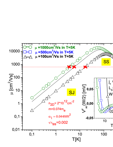
Figure 11: (color online) Mobility, $\mu$, as a function of temperature, $T$, for three different low-$T$ $\mu$’s. In inset, the spin accumulation ($V^{y}_{ac}$) vs. $T$. The side jump contribution to $V^{y}_{ac}$ dominates for low $T$. For increasing $T$, the lower temperature red cross corresponds to the $T$ where the sign of $V^{y}_{ac}$ starts to be controlled by skew scattering, the higher temperature red cross to the place where side jump dominates again.

As we mentioned before, it is possible to distinguish between side jump and skew scattering contributions to the spin accumulation because they scale differently with mobility. We have proposed an experiment to distinguish between these two contributions in a study of the temperature dependence of $\sigma^{SH}_{yx}$ or spin accumulation $V^{x}_{ac}=-V^{y}_{ac}$, where the last equality stems from the fact that the transverse resistivity elements are odd under exchange of spatial coordinates i.e. $\rho^{xy}=-\rho^{yx}$. Fig. (11) presents the behavior of mobility versus temperature for experimentally attainable samples. Due to different scattering mechanisms, the mobility scales non-monotonically with the temperature. Hence $\mu$ will grow as $T^{3/2}$ for low $T$ as a result of scattering from ionized impurities and will decrease as $T^{-3/2}$ for larger $T$ due to phonon scattering. It is thus possible to observe two changes of sign of $V^{y}_{ac}$ moving from low to high $T$s. $\mu=1/(AT^{-3/2}+BT^{3/2})$, where $A$ was found from the low-$T$ mobility and $B$ was fixed by a room temperature mobility of 0.3 m²/Vs for AlGaAs. At low $T$ the mobility is low and the side jump contribution to $V^{y}_{ac}$ dominates. With increasing $T$, the first cross designates the point where the skew scattering begins to dominate, and the second cross, at higher $T$, is the point where the side jump takes control of the sign of $V^{y}_{ac}$ again. Even if the sign change is not detected, by measuring whether $V^{y}_{ac}$ increases or decreases as $\mu$ increases with changing $T$ it should possible to tell whether side jump or skew scattering dominates. Notice that the values of parameters for the theoretical curve designated by circles are exactly the same as the values reported for the samples in the recent experiments Sih et al. (2005) on a [110] QW. The samples with lower mobilities can be easily obtained by additional doping with Si inside the quantum well.

V Influence of Rashba type spin-orbit interaction on Spin-Coulomb drag

So far, the influence of the Coulomb interaction on the intrinsic spin Hall effect has not been analyzed. The issue is more complex than the problem presented in Section IV i.e. the study of the influence of spin-Coulomb drag on the extrinsic spin Hall effect. The main difference between the problem with impurities and the problem that considers spin-orbit interaction coming from the band structure is that the latter usually does not conserve the $z$-component of spin. The general form of intrinsic spin-orbit interactions in 2D is:

$$H_{b}=-\frac{1}{2}{\vec{b}}({\vec{k}})\cdot{\vec{\sigma}}$$ (60)

where $\vec{\sigma}$ is the vector of the Pauli matrices and $\vec{b}(\vec{k})$ is the intrinsic spin-orbit field. Due to time reversal symmetry this field needs to fulfill the following condition: $\vec{b}(\vec{k})=-\vec{b}(-\vec{k})$. For example for the simplest model describing the spin-orbit interactions in a 2DEG oriented in [001] direction one hasBychkov and Rashba (1984):

$$\vec{b}(\vec{k})=2\alpha\vec{\hat{z}}\times\vec{k}$$ (61)

where $\vec{\hat{z}}$ is the unit vector in z direction and $\alpha$ is the spin-orbit coupling strength. This model is known in literature as the Rashba model Bychkov and Rashba (1984). For 2DHG, the Luttinger Hamiltonian for low densities can be simplified by taking into account only the heavy-hole band Winkler (2000); Schliemann and Loss (2005). This gives

$$H_{2DHG}=i\alpha_{h}(k^{3}_{-}\sigma_{+}-k^{3}_{+}\sigma_{-})\,.$$ (62)

Obviously, these Hamiltonians do not conserve the $z$-component of spin and therefore the simple approach presented in Section IV can not be applied. The main complication is that we need to consider the whole density matrix (also the off-diagonal terms) in the Boltzmann approach. However, the Rashba model (at least for the standard definition of spin-current Shi et al. (2006)) gives zero spin-Hall conductivity Inoue et al. (2004); Mishchenko et al. (2004); Dimitrova (2005); Raimondi and Schwab (2005); Khaetskii (2006); Hankiewicz and Vignale (2008) so we do not expect that this result will be further modified by e-e interactions. On the other hand, for the cubic spin-orbit models, vertex corrections are not important and the spin-Hall conductivity is of the order of $e^{2}/\hbar$. In this case, our expectation is that the spin-Hall conductivity, being non-universal, will be reduced by spin-Coulomb drag. However, there has not been yet the calculations which would quantitatively address this problem.

So far the only studied problem was the influence of spin-orbit interactions on the spin-Coulomb drag Tse and Sarma (2007). Diagrammatic calculations Tse and Sarma (2007), suggest that the spin-Coulomb drag is actually enhanced by spin-orbit interaction of the Rashba type, at least in the weak scattering regime. The correction is simply additive to what we would expect from microscopic calculations of spin-Coulomb drag without spin-orbit interaction D’Amico and Vignale (2000). It has the form $3(\gamma_{int}^{*})^{2}$ where $\gamma_{int}^{*}=\alpha m_{e}/(\upsilon_{F}m)$ where $\upsilon_{F}$ is the Fermi velocity. There is still much room of course for more detailed studies of the interplay between spin-orbit interaction and spin Coulomb drag. Recently, Weber et al. Weber et al. (2007) have undertaken experimental studies of the relaxation of a spin grating in a two-dimensional electron gas oriented in such a way that the spin-orbit interaction is relevant. A theoretical study by Weng et al.,Weng et al. (2008) which takes into account both spin-orbit coupling and electron-electron interaction concludes that the spin Coulomb drag will still be visible as a reduction of the spin diffusion constant. The latter is still determined from the initial decay rate of the amplitude of the spin grating, but the full time evolution of the amplitude involves two different spin relaxation times for in-plane and out-of-plane dynamics respectively.

VI Evolution of spin-Hall effect

As we showed in previous Sections, the spin-Hall effect has various contributions. Therefore, it is in place to compare the importance of different mechanisms contributing to the spin-Hall conductivity as a function of $\hbar\tau/m$. We chose $\hbar\tau/m$ as a SHE evolution parameter for two reasons (1) it has a dimension of a squared length and can be directly compared with the strength of the spin-orbit coupling $\alpha\hbar$ (2) $\hbar\tau/m$ can be easily connected with the mobility. When $\hbar\tau/m$ is expressed in $\AA^{2}$ it is approximately equal $6\mu$, where $\mu$ is the mobility in cm²/V.s.

In a d.c. limit we can distinguish three different regimes Onoda et al. (2006): (1) ultraclean regime where $\frac{\hbar}{\tau}\ll E_{so}$, where $E_{so}$ is the spin-orbit energy scale defined as $E_{so}=E_{F}(\alpha\hbar/a_{B}^{2})$, $a_{B}$ is the effective Bohr radius (2) clean regime characterized by inequality $E_{so}\ll\frac{\hbar}{\tau}\ll E_{F}$, where $E_{F}$ is the Fermi energy, (3) the dirty regime in which $\frac{\hbar}{\tau}>E_{F}$. In terms of $\hbar\tau/m$ these three regimes correspond to (1) $\frac{\hbar\tau}{m}\gg\frac{a_{B}^{4}}{\alpha\hbar}$ (ultraclean), (2) $a_{B}^{2}\ll\frac{\hbar\tau}{m}\ll\frac{a_{B}^{4}}{\alpha\hbar}$ (clean) and (3) $\frac{\hbar\tau}{m}<a_{B}^{2}$ (dirty) where we assumed $n=a_{B}^{-3}$. On top of these limits we need to know the relative importance of the skew scattering and side jump contributions to the spin-Hall conductivity. Let us therefore recall the final formulas for the skew scattering:

$$\sigma^{ss}=10^{-3}\frac{\sigma_{D}}{1+\gamma\tau}$$ (63)

and side jump spin-Hall conductivities:

$$\sigma^{sj}=-2\alpha ne^{2}.$$ (64)

The ratio of these two conductivities is:

$$\frac{\sigma^{sj}}{\sigma^{ss}}\approx 3\times 10^{2}\frac{\alpha\hbar[\AA^{2}]}{\mu[cm^{2}/V.s]}$$ (65)

where we used the connection between mobility and $\hbar\tau/m$. Also, in the above formula $\alpha\hbar$ is in units of Ų while $\mu$ is in cm²/V.s. The side jump and skew scattering contributions have the same magnitude when: $\frac{\hbar\tau}{m}=2\times 10^{3}\alpha\hbar$. As we already mentioned the skew scattering contribution scales with the mobility and therefore will dominate the ultraclean regime, where this quantity is the largest. The skew scattering contribution is cut-off by spin-Coulomb drag when $\gamma\gg 1/\tau$ and the cut-off value of spin-conductivity is $\sigma_{cut}^{ss}=10^{-3}\frac{ne^{2}}{m\gamma}$. Intrinsic contribution (if it is not zero, like in a Rashba model) dominates in a clean regime. As was shown theoretically Bernevig and Zhang (2005), the vertex corrections connected with disorder are zero for p-doped semiconductors and the spin-Hall conductivity is of the order of $e^{2}/\hbar$ and therefore much larger than the side-jump contribution. For example for typical 2D semiconducting hole gases with densities (10¹¹cm^-2), side jump contribution is around thousand times smaller than intrinsic one. Therefore in the scenario where the skew-scattering regime passes to the side jump regime the scale $2\times 10^{3}\alpha\hbar$ must be larger than $\frac{a_{B}^{4}}{\alpha\hbar}$. For doped semiconductors, for example GaAs, the effective Bohr radius is 100Å, so we have $\frac{a_{B}^{4}}{\alpha\hbar}\approx 4\times 10^{6}\alpha\hbar\gg 2\times 10^{3}\alpha\hbar$. Therefore we will have a direct transition from the skew scattering to the intrinsic regime. However, there are two options to observe the side-jump effect: (i) the intrinsic contribution is zero (like in Rashba model), then side-jump could be observed in the clean limit (ii) the mobility is decreased by changing the temperature and the side-jump contribution could be observed in ultraclean regime as we mentioned in Section V (see Fig. (11)). In the dirty regime the spin-Hall conductivity diminishes to zero. The scenario of evolution of spin-Hall conductivity in semiconductors with non-zero intrinsic contribution is presented in Fig. (12). In contrast, if one adopts Eq. (63) and Eq. (64) to describe the spin-Hall effect in metals, one finds that the skew scattering term would evolve into side-jump contribution for $\hbar\tau/m^{*}=10^{3}\alpha$ and the intrinsic effect will eventually appear for $\hbar\tau/m^{*}=a_{B}^{4}/(\alpha\hbar)$ in the clean regime. For parameters typical for Pt, the side jump and intrinsic contributions are of the same order and dominant. Therefore further calculations (including the complexity of band structure) and experiments are needed to distinguish between various mechanisms contributing to SHE in metals.

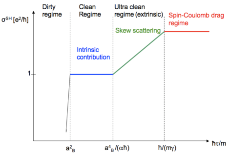
Figure 12: (color online) Evolution of the spin-Hall effect as a function of $\hbar\tau/m$ assuming that an electron-impurity scattering potential has the form of the screened Coulomb potential. The side jump could be observed in an ultraclean regime if we decrease the mobility by for example the tuning of temperature.

VII Summary

In this review we have summarized the current status of the knowledge concerning the extrinsic spin Hall effect and the spin Coulomb drag effect, and the relation between them. Careful readers will notice that there are still plenty of open questions and unsolved problems.

From the theoretical point of view, perhaps the most urgent open challenge is the calculation of the influence of the spin-Coulomb drag on the intrinsic spin Hall effect. From the experimental point of view, it would be interesting to see time-resolved studies of the spin Hall effect, possibly conducted by spin-grating techniques Weber et al. (2005, 2007) or by optical spin injection techniques Zhao et al. (2006); Stern et al. (2008). Furthermore, a direct detection of the influence of the spin-Coulomb drag on the spin-Hall effect and an experimental verification of the theoretical predictions of Section IV would be of great interest. Finally, a full description of the interplay between spin-orbit coupling and spin Coulomb drag remains an open challenge, particularly at the experimental level.

Acknowledgements. This work was supported by NSF Grant No. DMR-0705460.

References

- Awschalom and Flatte (2007) D. D. Awschalom and M. E. Flatte, Nature Physics 3, 153 (2007).
- Engel et al. (2007) H.-A. Engel, E. I. Rashba, and B. I. Halperin, Handbook of Magnetism and Advanced Magnetic Materials (John Wiley & Sons Ltd, Chichester, UK, 2007).
- Murakami (2005) S. Murakami, Adv. in Solid State Phys. 45, 197 (2005).
- Karplus and Luttinger (1954) R. Karplus and J. M. Luttinger, Phys. Rev. B 95, 1154 (1954).
- Smit (1955) J. Smit, Physica 21, 877 (1955).
- Smit (1958) J. Smit, Physica 24, 39 (1958).
- Ber (a) L. Berger Phys. Rev. B 2, 4559 (1970).
- Ber (b) L. Berger Phys. Rev. B 5, 1862 (1972).
- Lyo and Holstein (1972) S. K. Lyo and T. Holstein, Phys. Rev. Lett. 29, 423 (1972).
- Noziéres and Lewiner (1973) P. Noziéres and C. Lewiner, J. Phys. (Paris) 34, 901 (1973).
- Crépieux and Bruno (2001) A. Crépieux and P. Bruno, Phys. Rev. B 64, 014416 (2001).
- Jungwirth et al. (2002) T. Jungwirth, Q. Niu, and A. H. MacDonald, Phys. Rev. Lett. 88, 207208 (2002).
- Onoda and Nagaosa (2003) M. Onoda and N. Nagaosa, Phys. Rev. Lett. 90, 206601 (2003).
- Dugaev et al. (2005) V. K. Dugaev, P. Bruno, M. Taillefumier, B. Canals, and C. Lacroix, Phys. Rev. B 71, 224423 (2005).
- Nunner et al. (2007) T. S. Nunner et al., Phys. Rev. B 76, 235312 (2007).
- Sinitsyn (2008) N. A. Sinitsyn, J. Phys. Cond. Matt. 20, 023201 (2008).
- Dyakonov and Perel (1971a) M. I. Dyakonov and V. I. Perel, Phys. Lett. A 35, 459 (1971a).
- Dyakonov and Perel (1971b) M. I. Dyakonov and V. I. Perel, Zh. Eksp. Ter. Fiz. 13, 657 (1971b).
- Hirsch (1999) J. E. Hirsch, Phys. Rev. Lett. 83, 1834 (1999).
- Zhang (2000) S. Zhang, Phys. Rev. Lett. 85, 393 (2000).
- Murakami et al. (2003) S. Murakami, N. Nagaosa, and S.-C. Zhang, Science 301, 1348 (2003).
- Sinova et al. (2004) J. Sinova, D. Culcer, Q. Niu, N. A. Sinitsyn, T. Jungwirth, and A. H. MacDonald, Phys. Rev. Lett. 92, 126603 (2004).
- Culcer et al. (2004) D. Culcer, J. Sinova, N. A. Sinitsyn, T. Jungwirth, A. H. MacDonald, and Q. Niu, Phys. Rev. Lett. 93, 046602 (2004).
- Schliemann and Loss (2004) J. Schliemann and D. Loss, Phys. Rev. B 69, 165315 (2004).
- Burkov et al. (2004) A. A. Burkov, A. S. Nunez, and A. H. MacDonald, Phys. Rev. B 70, 155308 (2004).
- Murakami et al. (2004) S. Murakami, N. Nagaosa, and S.-C. Zhang, Phys. Rev. B 69, 235206 (2004).
- Murakami (2004) S. Murakami, Phys. Rev. B 69, 241202(R) (2004).
- Sinitsyn et al. (2004) N. A. Sinitsyn, E. M. Hankiewicz, W. Teizer, and J. Sinova, Phys. Rev. B 70, 081312(R) (2004).
- Inoue et al. (2004) J. I. Inoue, G. E. W. Bauer, and L. W. Molenkamp, Phys. Rev. B 70, 041303(R) (2004).
- Mishchenko et al. (2004) E. G. Mishchenko, A. V. Shytov, and B. I. Halperin, Phys. Rev. Lett. 93, 226602 (2004).
- Schliemann and Loss (2005) J. Schliemann and D. Loss, Phys. Rev. B 71, 085308 (2005).
- Dimitrova (2005) O. V. Dimitrova, Phys. Rev. B 71, 245327 (2005).
- Raimondi and Schwab (2005) R. Raimondi and P. Schwab, Phys. Rev. B 71, 033311 (2005).
- Khaetskii (2006) A. Khaetskii, Phys. Rev. B 73, 115323 (2006).
- Duckheim and Loss (2006) M. Duckheim and D. Loss, Nature Physics 2, 195 (2006).
- Gorini et al. (2008) C. Gorini, P. Schwab, M. Dzierzawa, and R. Raimondi, Phys. Rev. B 78, 125327 (2008).
- Tse and Sarma (2006) W. K. Tse and S. D. Sarma, Phys. Rev. B 74, 245309 (2006).
- Hankiewicz and Vignale (2008) E. M. Hankiewicz and G. Vignale, Phys. Rev. Lett. 100, 026602 (2008).
- Kato et al. (2004) Y. K. Kato, R. C. Myers, A. C. Gossard, and D. D. Awschalom, Science 306, 1910 (2004).
- Sih et al. (2005) V. Sih et al., Nature Physics 1, 31 (2005).
- Wunderlich et al. (2005) J. Wunderlich et al., Phys. Rev. Lett. 94, 047204 (2005).
- Stern et al. (2006) N. P. Stern et al., Phys. Rev. Lett. 97, 126603 (2006).
- Stern et al. (2008) N. P. Stern, D. W. Steuerman, S. Mack, A. C. Gossard, and D. D. Awschalom, Nature Physics 4, 843 (2008).
- Zhao et al. (2006) H. Zhao et al., Phys. Rev. Lett. 96, 246601 (2006).
- Hankiewicz et al. (2004) E. M. Hankiewicz, L. W. Molenkamp, T. Jungwirth, and J. Sinova, Phys. Rev. B 70, 241301(R) (2004).
- Brüne et al. (2008) C. Brüne, A. Roth, E. G. Novik, M. König, H. Buhmann, E. M. Hankiewicz, W. Hanke, J. Sinova, and L. W. Molenkamp (2008), eprint arXiv:0812.3768.
- Gui et al. (2004) Y. S. Gui et al., Phys. Rev. B 70, 115328 (2004).
- Bychkov and Rashba (1984) Y. A. Bychkov and E. I. Rashba, J. Phys. C 17, 6039 (1984).
- Hankiewicz et al. (2005) E. M. Hankiewicz, J. Li, T. Jungwirth, Q. Niu, S.-Q. Shen, and J. Sinova, Phys. Rev. B 72, 155305 (2005).
- Valenzuela and Tinkham (2006) S. O. Valenzuela and M. Tinkham, Nature 442, 176 (2006).
- (51) K. C. Weng, N. Chandrasekhar, C. Miniatura, and B.-G. Englert, eprint arXiv:0804.0096.
- Shchelushkin and Brataas (2005) R. V. Shchelushkin and A. Brataas, Phys. Rev. B 72, 073110 (2005).
- Tanaka et al. (2008) T. Tanaka, H. Kontani, M. Naito, T. Naito, D. S. Hirashima, K.Yamada, and J. Inoue, Phys. Rev. B 77, 165117 (2008).
- (54) G. Y. Guo, S. Murakami, T.-W. Chen, and N. Nagaosa, eprint arXiv:0705.0409v4.
- Kane and Mele (2005) C. L. Kane and E. J. Mele, Phys. Rev. Lett. 95, 226801 (2005).
- Bernevig and Zhang (2006) B. A. Bernevig and S.-C. Zhang, Phys. Rev. Lett. 96, 106802 (2006).
- Bernevig et al. (2006) B. A. Bernevig, T. L. Hughes, and S.-C. Zhang, Science 314, 1757 (2006).
- König et al. (2007) M. König, S. Wiedmann, C. Brüne, A. Roth, H. Buhmann, L. W. Molenkamp, X. L. Qi, and S.-C. Zhang, Science 318, 766 (2007).
- König et al. (2008) M. König, H. Buhmann, L. W. Molenkamp, T. L. Hughes, C. X. Liu, X. L. Qi, and S.-C. Zhang, J. of Phys. Soc. of Japan 77, 031007 (2008).
- Wu et al. (2006) C. Wu, B. A. Bernevig, and S.-C. Zhang, Phys. Rev. Lett. 96, 106401 (2006).
- Xu and Moore (2006) C. Xu and J. Moore, Phys. Rev. B 73, 045322 (2006).
- D’Amico and Vignale (2000) I. D’Amico and G. Vignale, Phys. Rev. B 62, 4853 (2000).
- Flensberg et al. (2001) K. Flensberg, T. S. Jensen, and N. A. Mortensen, Phys. Rev. B 64, 245308 (2001).
- D’Amico and Vignale (2001) I. D’Amico and G. Vignale, Europhysics Lett. 55, 566 (2001).
- D’Amico and Vignale (2002) I. D’Amico and G. Vignale, Phys. Rev. B 65, 85109 (2002).
- D’Amico and Vignale (2003) I. D’Amico and G. Vignale, Phys. Rev. B 68, 045307 (2003).
- Vignale (2007) G. Vignale, Manipulating Quantum Coherence in Solid State Systems, M. E. Flatte and I. Tifrea (editors) (Springer, Berlin, 2007).
- Badalyan et al. (2008) S. M. Badalyan, C. S. Kim, and G. Vignale, Phys. Rev. Lett. 100, 016603 (2008).
- Weber et al. (2005) C. P. Weber, N. Gedik, J. E. Moore, J. Orenstein, J. Stephens, and D. D. Awschalom, Nature 437, 1330 (2005).
- Engel et al. (2005) H. A. Engel, B. I. Halperin, and E. Rashba, Phys. Rev. Lett. 95, 166605 (2005).
- Hankiewicz and Vignale (2006) E. M. Hankiewicz and G. Vignale, Phys. Rev. B 73, 115339 (2006).
- Mott and Massey (1964) N. F. Mott and H. S. W. Massey, The Theory of Atomic Collisions (Oxford University Press, 1964).
- Foldy and Wouthuysen (1950) L. L. Foldy and S. A. Wouthuysen, Phys. Rev. 78, 29 (1950).
- Winkler (2003) R. Winkler, Spin-orbit effects in two-dimensional electron and hole systems (Springer, 2003).
- Landau and Lifshitz (1964) L. D. Landau and E. M. Lifshitz, Course of Theoretical Physics, Vol. III. (Butterworth-Heinemann, Oxford, 1964).
- Kohn and Luttinger (1957) W. Kohn and J. M. Luttinger, Phys. Rev. 108, 590 (1957).
- Hankiewicz et al. (2006) E. M. Hankiewicz, G. Vignale, and M. Flatté, Phys. Rev. Lett. 97, 266601 (2006).
- Rojo (1999) A. G. Rojo, J. Phys. Cond. Mat. 11, R31 (1999).
- Kikkawa et al. (1997) J. M. Kikkawa, I. P. Smorchkova, N. Samarth, and D. D. Awschalom, Science 277, 1284 (1997).
- Kikkawa and Awschalom (1998) J. M. Kikkawa and D. D. Awschalom, Phys. Rev. Lett. 90, 4313 (1998).
- Giuliani and Vignale (2005) G. F. Giuliani and G. Vignale, Quantum Theory of the Electron Liquid (Cambridge University Press, UK, 2005).
- Tse et al. (2005) W.-K. Tse, J. Fabian, I. utic, and S. D. Sarma, Phys. Rev. B 72, 241303 (2005).
- Valet and Fert (1993) T. Valet and A. Fert, Phys. Rev. B 48, 7099 (1993).
- Winkler (2000) R. Winkler, Phys. Rev. B 62, 4245 (2000).
- Shi et al. (2006) J. Shi, P. Zhang, D. Xiao, and Q. Niu, Phys. Rev. Lett. 96, 076604 (2006).
- Tse and Sarma (2007) W.-K. Tse and S. D. Sarma, Phys. Rev. B 75, 045333 (2007).
- Weber et al. (2007) C. P. Weber et al., Phys. Rev. Lett. 98, 076604 (2007).
- Weng et al. (2008) M. Q. Weng, M. W. Wu, and H. L. Cui, J. App. Phys. 103, 063714 (2008).
- Onoda et al. (2006) S. Onoda, N. Sugimoto, and N. Nagaosa, Phys. Rev. Lett. 97, 126602 (2006).
- Bernevig and Zhang (2005) B. A. Bernevig and S.-C. Zhang, Phys. Rev. Lett. 95, 016801 (2005).