Subdiffusive behavior in a trapping potential: mean square displacement and velocity autocorrelation function

Abstract

A theoretical framework for analyzing stochastic data from single-particle tracking in complex or viscoelastic materials and under the influence of a trapping potential is presented. Starting from a generalized Langevin equation we found explicit expressions for the two-time dynamics of the tracer particle. The mean square displacement and the velocity autocorrelation function of the diffusing particle are given in terms of the time lag. In particular, we investigate the subdiffusive case. The exact solutions are discussed and the validity of usual approximations are examined.

I Introduction

The viscoelastic properties of complex fluids, like polymers, colloids and biological materials, can be derived from the dynamics of individual spherical particles embedded in it Wai ; Val . Particle tracking microrheology experiments Wai ; Val ; Yam ; Lau ; Ma95 ; Ma97 ; Qian ; Lev are based on the observation of the motion of individual tracer particles. In a typical microrheology experiment, particle positions are recorded in the form of a time sequence and information about the dynamics is essentially extracted by measuring the mean square displacement of the probe particles LuSol ; Dan ; Gold . Based on a generalized Langevin equation with a memory function and assuming that inertial effects are negligible, Mason and coworkers Ma95 ; Ma97 have obtained a direct relation between the mean-square displacement of free tracer particles and the viscoelastic parameters of the environment. It has been recently noted that the fluid inertia and the resulting memory effects become increasingly important when high-resolution experiments are performed Luk1 .

On the other hand, optical traps are increasingly used for position detection, with a wide range of applications in physics and biology Yam ; Neu ; Luk2 ; Ata ; Fis ; Cas . In an optical trap, the interaction between the laser and the trapped object can be approximated by a harmonic potential Den . However, the use of a trapping complicates the analysis of the obtained data, since the interactions with the viscoelastic environment overlaps with the influence of the trapping force Wai ; Luk1 . For example, it has been noticed that neglecting memory effects leads to calibration errors of optical traps Luk2 .

It is now well established that when particles diffuse through a soft complex fluids or biological materials, they exhibit anomalous subdiffusive behaviors Val ; Dan ; Bra ; Gui ; Tol . In this situation, the mean-square displacement exhibit a slow relaxation with the presence power-law decay in the range of large times. A theoretical complete description of the behavior of a particle in a complex medium and subjected to a harmonic potential can be formulated in terms of the generalized Langevin equation (GLE) containing a memory function WaTo ; Porr ; Pot ; VD . In a recent paper VD , we have obtained analytical expressions for the evolution of mean values and variances in terms of Mittag-Leffler functions. However, from an experimental point of view it is necessary to get expressions for the two-times correlation functions. For instance, the mean square displacement (MSD) can be expressed as

$$\rho(\tau)=\lim_{t\to\infty}\langle\left(X(t+\tau)-X(t)\right)^{2}\rangle\,,$$ (1)

where $|X(t+\tau)-X(t)|$ is the particle displacement between two time points, $t$ denote the absolute time while $\tau$ is the so-called lag time Metz . Alternative information about the experimentally observed diffusive behavior can be extracted from the normalized velocity autocorrelation function (VACF) Qian1 , defined as Porr ; VD

$$C_{V}(\tau)=\lim_{t\to\infty}\frac{\langle V(t+\tau)V(t)\rangle}{\langle V^{2}(t)\rangle}\,.$$ (2)

Then, to calculate the MSD and the VACF one must know the behavior of the two-time correlations $\langle X(t+\tau)X(t)\rangle$ and $\langle V(t+\tau)V(t)\rangle$. In what follows we will investigate the behavior of the MSD (1) and VACF (2) for harmonically bounded particle immersed in a viscoelastic environment. For this purpose, in Sec. 2 we present the corresponding generalized Langevin equation (GLE). The two-time dynamics is obtained, which enable us to calculate the MSD and VACF for arbitrary memory kernels. Section 3 is devoted to the study of the subdiffusive case. The analytical solutions are given and compared with the overdamped approximation. Finally, a Summary of our results is presented in Sec.4 .

II Diffusion in a harmonic well

II.1 Formal solution for the GLE

In what follows we consider the dynamics of a test particle of mass $m$, immersed in a complex or viscoelastic environment and simultaneously bounded in a harmonic potential well. The resulting motion can be described by the following GLE

$$m\ddot{X}(t)+m\int_{0}^{t}dt^{\prime}\gamma(t-t^{\prime})\dot{X}(t^{\prime})+m\omega_{0}^{2}X=F(t)\,,$$ (3)

where $\omega_{0}$ is the frequency of the trap, $\gamma(t)$ is the dissipative memory kernel, and the internal noise $F(t)$ is a zero-centered and stationary random force with correlation function

$$\langle F(t)F(t^{\prime})\rangle=C(|t-t^{\prime}|)=C(\tau)\,.$$ (4)

The integral term in (3) represents the dependence of the viscous force on the velocity history and the memory kernel $\gamma(t)$ is related to the noise correlation function $C(t)$ via the second fluctuation-dissipation theorem Zwa

$$C(t)=k_{B}T\,m\,\gamma(t)\,,$$ (5)

where $T$ is the absolute temperature, and $k_{B}$ is the Boltzmann constant.

In what follows we consider the one-dimensional case, but our results can be easily extrapolated to the two or three dimensional case. The Langevin equation (3) can be formally solved by means of the Laplace transformation. Taking into account the deterministic initial conditions $x_{0}=X(0)$ and $v_{0}=\dot{X}(0)$, the evolution of the Laplace transform of the position $X(t)$ reads

$$\widehat{X}(s)=x_{0}\left(\frac{1}{s}-\omega_{0}^{2}\,\widehat{I}(s)\right)+\left(v_{0}+\frac{1}{m}\widehat{F}(s)\right)\widehat{G}(s)\,,$$ (6)

where $\widehat{F}(s)$ is the Laplace transform of the noise. The relaxation function $G(t)$ is the Laplace inversion of

$$\widehat{G}(s)=\frac{1}{s^{2}+s\widehat{\gamma}(s)+\omega_{0}^{2}}\,,$$ (7)

where $\widehat{\gamma}(s)$ is the Laplace transform of the damping kernel, and

$$\widehat{I}(s)=\frac{\widehat{G}(s)}{s}\,,$$ (8)

is the Laplace transform of

$$I(t)=\int_{0}^{t}dt^{\prime}G(t^{\prime})\,.$$ (9)

On the other hand, the Laplace transform of the velocity $V(t)=\dot{X}(t)$ satisfies that

$$\widehat{V}(s)=\left(v_{0}+\frac{1}{m}\widehat{F}(s)\right)\widehat{g}(s)-x_{0}\,\omega_{0}^{2}\,\widehat{G}(s)\,,$$ (10)

where

$$\widehat{g}(s)=s\,\widehat{G}(s).$$ (11)

From Eqs. (6) and (10) a formal expression for the displacement $X(t)$ and the velocity $V(t)$ can be written as

$$X(t) = \langle X(t)\rangle+\frac{1}{m}\int_{0}^{t}dt^{\prime}G(t-t^{\prime})F(t^{\prime})\,,$$ (12)

$$V(t) = \langle V(t)\rangle+\frac{1}{m}\int_{0}^{t}dt^{\prime}g(t-t^{\prime})F(t^{\prime})\,,$$ (13)

where

$$\langle X(t)\rangle = x_{0}\left(1-\omega_{0}^{2}\,I(t)\right)+v_{0}\,G(t)\,,$$ (14)

$$\langle V(t)\rangle = v_{0}\,g(t)-x_{0}\,\omega_{0}^{2}\,G(t)\,,$$ (15)

are the position and velocity mean values evolution, respectively.

II.2 Expressions for the MSD and VACF

To calculate the two-time properties of the dynamical variables involved in the expressions of the MSD (1) and VACF (2) we will make use of the double Laplace transform technique Pot . Then, from (6) and (10) we have

$$\langle\widehat{X}(s)\widehat{X}(s^{\prime})\rangle = x_{0}^{2}\,\widehat{\chi}(s)\widehat{\chi}(s^{\prime})+v_{0}^{2}\,\widehat{G}(s)\widehat{G}(s^{\prime})$$ (16)

$$+ x_{0}\,v_{0}\,(\widehat{\chi}(s)\widehat{G}(s^{\prime})+\widehat{\chi}(s^{\prime})\widehat{G}(s))$$

$$+ \frac{1}{m^{2}}\,\widehat{G}(s)\widehat{G}(s^{\prime})\langle\widehat{F}(s)\widehat{F}(s^{\prime})\rangle\,,$$

$$\langle\widehat{V}(s)\widehat{V}(s^{\prime})\rangle = v_{0}^{2}\,\widehat{g}(s)\widehat{g}(s^{\prime})+x_{0}^{2}\,\omega_{0}^{4}\,\widehat{G}(s)\widehat{G}(s^{\prime})$$ (17)

$$- x_{0}\,v_{0}\,\omega_{0}^{2}\,(\widehat{g}(s)\widehat{G}(s^{\prime})+\widehat{g}(s^{\prime})\widehat{G}(s))$$

$$+ \frac{1}{m^{2}}\,\widehat{g}(s)\widehat{g}(s^{\prime})\langle\widehat{F}(s)\widehat{F}(s^{\prime})\rangle\,,$$

where

$$\widehat{\chi}(s)=\frac{1}{s}-\omega_{0}^{2}\widehat{I}(s)\,$$ (18)

is the Laplace transform of $\chi(t)=1-\omega_{0}^{2}I(t)$.

In the Appendix we show how the last term of Eqs. (16) and (17) can be calculated. Inserting expressions (51) and (52) into (16) and (17) and making a double Laplace inversion, we arrive at

$$\langle X(t)X(t^{\prime})\rangle = x_{0}^{2}\,\chi(t)\chi(t^{\prime})+(v_{0}^{2}-\frac{k_{B}T}{m})G(t)G(t^{\prime})+x_{0}\,v_{0}\,(\chi(t)G(t^{\prime})+\chi(t^{\prime})G(t))$$ (19)

$$+ \frac{k_{B}T}{m}\left(I(t)+I(t^{\prime})-I(|t-t^{\prime}|)\right)-\frac{k_{B}T}{m}\,\omega_{0}^{2}\,I(t)I(t^{\prime})\,,$$

$$\langle V(t)V(t^{\prime})\rangle = \frac{k_{B}T}{m}\,g(|t-t^{\prime}|)+(v_{0}^{2}-\frac{k_{B}T}{m})g(t)g(t^{\prime})+\omega_{0}^{2}\,(x_{0}^{2}\omega_{0}^{2}-\frac{k_{B}T}{m})G(t)G(t^{\prime})$$ (20)

$$- x_{0}v_{0}\,\omega_{0}^{2}\,(g(t)G(t^{\prime})+g(t^{\prime})G(t))$$

Finally, by considering time lags $\tau>0$, from (19) and (20) we have

$$\langle\left(X(t+\tau)-X(t)\right)^{2}\rangle = \frac{2k_{B}T}{m}\,I(\tau)-2x_{0}v_{0}\omega_{0}^{2}\left(G(t+\tau)-G(t)\right)\left(I(t+\tau)-I(t)\right)$$ (21)

$$+ (v_{0}^{2}-\frac{k_{B}T}{m})\left(G(t+\tau)-G(t)\right)^{2}+\omega_{0}^{2}\,(x_{0}^{2}\omega_{0}^{2}-\frac{k_{B}T}{m})\left(I(t+\tau)-I(t)\right)^{2}\,,$$

$$\langle V(t+\tau)V(t)\rangle = \frac{k_{B}T}{m}\,g(\tau)+(v_{0}^{2}-\frac{k_{B}T}{m})g(t+\tau)g(t)+\omega_{0}^{2}\,(x_{0}^{2}\omega_{0}^{2}-\frac{k_{B}T}{m})G(t+\tau)G(t)$$

$$- x_{0}\,v_{0}\,\omega_{0}^{2}\,\left(g(t+\tau)G(t)+g(t)G(t+\tau)\right)\,.$$

Note that the analytical expressions (21) and (II.2) are exact and valid for all absolute times $t$ and time lags $\tau$. However, to evaluate the MSD (1) and VACF (2) we must take the limit $t\rightarrow\infty$. In this case, these expressions could be simplified as follows. Taking into account the usual assumption that the time-dependent frictional coefficient $\gamma(t)$ goes to zero when $t\to\infty$ DV1 and using the final value theorem Spig one gets

$$\lim_{t\to\infty}\gamma(t)=\lim_{s\to 0}s\widehat{\gamma}(s)=0\,.$$ (23)

Noticing that the Laplace transform of the relaxation function $I(t)$ defined through Eq. (8) is

$$\widehat{I}(s)=\frac{s^{-1}}{s^{2}+s\,\widehat{\gamma}(s)+\omega_{0}^{2}}\,,$$ (24)

the application of the final value theorem and the use of condition (23) yields DV1

$$I(\infty) = 1/{\omega_{0}^{2}}\,,$$ (25)

and using (8) and (11) gives

$$G(\infty) = g(\infty)=0\,.$$ (26)

Applying these conditions in order to take the limit $t\to\infty$ in (21) and (II.2), and using the definitions (1) and (2) one finally obtain the simpler expressions

$$\rho(\tau)=\frac{2k_{B}T}{m}I(\tau)\,,$$ (27)

and

$$C_{V}(\tau)=g(\tau)\,.$$ (28)

Taking into account (25) and (26), the equilibrium value of the MSD is given by

$$\rho(\infty)=\frac{2k_{B}T}{m\omega_{0}^{2}}\,,$$ (29)

while, as expected, the VACF decays to zero, i.e. $C_{V}(\infty)=0$.

It is worth pointing out that in experimental realizations the time lag is $\tau_{\text{min}}\leq\tau\leq\tau_{\text{max}}$, being $\tau_{\text{min}}$ the acquisition time interval and $\tau_{\text{max}}$ the measurement time. Moreover, if $N$ is the number of steps $n$ taken at intervals $\tau_{\text{min}}$, only small values of $n$ $(n<N/10)$ are used. Therefore, it is important to obtain valid expressions for all observational time scales instead of getting only its behavior to large times.

To conclude this section, we will find the extension for a trapped particle of the widely used Mason formula Ma95 ; Ma97 . Taking the Laplace transform of (27) and using the definition (24) of the relaxation function $I(t)$, one gets

$$s\widehat{\gamma}(s)=\frac{2k_{B}T}{m}\frac{1}{s\,\widehat{\rho}(s)}-s^{2}-\omega_{0}^{2}\,,$$ (30)

which gives a direct relation between the mean-square displacement of the particle and the memory kernel, from which the viscoelastic shear moduli of the medium can be obtained Wai .

III Subdiffusive behavior

Notice that the previous results are valid for any memory kernel that satisfy condition (23). On the other hand, it is well known that in the absence of active transport the dynamics of the particle in a viscoelastic fluid or complex media is subdiffusive and thus the stochastic process presents a long-time tail noise. The most utilized model to reproduce a subdiffusive behavior is characterized by a noise correlation function exhibiting a power-law time decay Wa1 ; Lu2 ; VD :

$$C(t)=C_{\lambda}\,\frac{t^{-\lambda}}{\Gamma(1-\lambda)},$$ (31)

where $\Gamma(z)$ is the Gamma function Po . The exponent $\lambda$ is taken as $0<\lambda<1$ and the proportionality coefficient $C_{\lambda}$ is independent of time but can depends on the exponent $\lambda$.

Using the fluctuation-dissipation relation (5), the memory kernel $\gamma(t)$ can be written as

$$\gamma(t)=\frac{\gamma_{\lambda}}{\Gamma(1-\lambda)}\,t^{-\lambda}\,,$$ (32)

where $\gamma_{\lambda}=C_{\lambda}/k_{B}T$. Then, its Laplace transform reads

$$\widehat{\gamma}(s)=\gamma_{\lambda}\,s^{\lambda-1}\,.$$ (33)

In this situation, the Laplace transform of the relaxation function $\widehat{I}(s)$ reads

$$\widehat{I}(s)=\frac{s^{-1}}{s^{2}+\gamma_{\lambda}\,s^{\lambda}+\omega_{0}^{2}}\,.$$ (34)

The complete temporal behavior of the relaxation functions $I(t)$, $G(t)$ and $g(t)$ was previously obtained by us in Ref. VD . Using those results in (27) and (28) we have

$$\rho(\tau) = \frac{2k_{B}T}{m}\,\sum_{k=0}^{\infty}\frac{(-1)^{k}}{k!}\,(\omega_{0}\tau)^{2k}\tau^{2}$$ (35)

$$\qquad\qquad\times\,E_{2-\lambda,3+\lambda k}^{(k)}(-\gamma_{\lambda}\,\tau^{2-\lambda})\,,$$

$$C_{V}(\tau) = \sum_{k=0}^{\infty}\frac{(-1)^{k}}{k!}\,(\omega_{0}\tau)^{2k}$$ (36)

$$\qquad\qquad\times\,E_{2-\lambda,1+\lambda k}^{(k)}(-\gamma_{\lambda}\,\tau^{2-\lambda})\,,$$

where $E_{\alpha,\beta}(y)$ is the generalized Mittag-Leffler function Po defined by the series expansion

$$E_{\alpha,\beta}(y)=\sum_{j=0}^{\infty}\frac{y^{j}}{\Gamma(\alpha j+\beta)},\quad\alpha>0,\quad\beta>0\,,$$ (37)

and $E_{\alpha,\beta}^{(k)}(y)$ is the derivative of the Mittag-Leffler function

$$E_{\alpha,\beta}^{(k)}(y)=\frac{d^{k}}{dy^{k}}E_{\alpha,\beta}(y)=\sum_{j=0}^{\infty}\frac{(j+k)!\,y^{j}}{j!\,\Gamma(\alpha(j+k)+\beta)}\,.$$ (38)

Using the series expansions (37) and (38) one can realize that the short times behavior of the MSD reads

$$\rho(\tau) \approx \frac{k_{B}T}{m}\,\left\{\tau^{2}-\frac{2\gamma_{\lambda}}{\Gamma(5-\lambda)}\,\tau^{4-\lambda}-\frac{\omega_{0}^{2}}{12}\,\tau^{4}\right\}\,,$$ (39)

where the first term shows that the particle undergoes ballistic motion when time is very small Wa2 . The second term comes from the influence of the viscoelastic medium while the third term corresponds to the fact that the particle begins to “see” the trap. The short times behavior of the VACF can be obtained in a similar way. In this case we get

$$C_{V}(\tau) \approx 1-\frac{\gamma_{\lambda}}{\Gamma(3-\lambda)}\,\tau^{2-\lambda}-\frac{\omega_{0}^{2}}{2}\,\tau^{2}\,.$$ (40)

On the other hand, for $\gamma_{\lambda}\,\tau^{2-\lambda}\gg 1$ the MSD and VACF can be obtained introducing the asymptotic behavior of the Mittag-Leffler function Po ,

$$E_{\alpha,\beta}(-y)\thicksim\frac{1}{y\,\Gamma(\beta-\alpha)}\,,\quad y>0$$ (41)

into Eqs. (35) and (36). After some calculations we have

$$\rho(\tau) \approx \frac{2k_{B}T}{m\omega_{0}^{2}}\left\{1-\,E_{\lambda}(-\frac{\omega_{0}^{2}}{\gamma_{\lambda}}\,\tau^{\lambda})\right\}\,,$$ (42)

$$C_{V}(\tau) \approx -\frac{1}{\omega_{0}^{2}}\,\frac{d^{2}}{d^{2}t}E_{\lambda}(-\frac{\omega_{0}^{2}}{\gamma_{\lambda}}\,\tau^{\lambda})\,,$$ (43)

where $E_{\lambda}(y)=E_{\lambda,1}(y)$ denotes the one parameter Mittag-Leffler function Po .

It is worth pointing out that these expressions can be also obtained discarding the inertial term $s^{2}$ in (34). In this case we get

$$\widehat{I}(s)=\frac{s^{-1}}{\gamma_{\lambda}\,s^{\lambda}+\omega_{0}^{2}}=\frac{1}{\omega_{0}^{2}}\left(\frac{1}{s}-\frac{s^{\lambda-1}}{s^{\lambda}+\omega_{0}^{2}/\gamma_{\lambda}}\right)\,,$$ (44)

and using that the Laplace transform of the Mittag-Leffler function Po

$$\int_{0}^{\infty}\,e^{-st}\,E_{\alpha}(-\gamma t^{\alpha})\,dt=\frac{s^{\alpha-1}}{s^{\alpha}+\gamma}\,,$$ (45)

one obtains expressions (42) and (43).

Finally, if $\tau^{\lambda}\gg\gamma_{\lambda}/\omega_{0}^{2}$ the behavior of the MSD and VACF can be obtained using again the approximation (41). In this case we get

$$\rho(\tau) \approx \frac{2k_{B}T}{m\omega_{0}^{2}}\left\{1-\frac{{\gamma_{\lambda}}}{\omega_{0}^{2}}\,\frac{1}{\Gamma(1-\lambda)}\,\tau^{-\lambda}\right\}\,,$$ (46)

$$C_{V}(\tau) \approx -\frac{{\gamma_{\lambda}}}{\omega_{0}^{4}}\,\frac{\lambda(\lambda+1)}{\Gamma(1-\lambda)}\,\tau^{-(\lambda+2)}\,,$$ (47)

showing a pure power law decay.

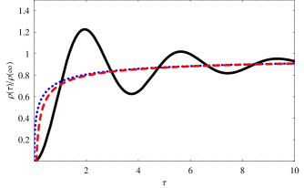
Figure 1: (color online) MSD vs. time lag for $\lambda=1/2$, $\gamma_{\lambda}=1$ and $\omega_{0}=1.4$. The solid line corresponds to the exact solution (35), the dotted line to the approximate solution (42) and the dashed line to the asymptotic behavior (46).

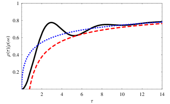
Figure 2: (color online) Idem Fig. 1 for $\omega_{0}=0.8$.

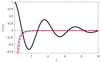
Figure 3: (color online) $C_{V}$ vs. time lag for $\lambda=1/2$, $\gamma_{\lambda}=1$ and $\omega_{0}=1.4$. The solid line corresponds to the exact solution (36), the dotted line to the approximate solution (43) and the dashed line to the asymptotic behavior (47).

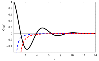
Figure 4: (color online) Idem Fig. 3 for $\omega_{0}=0.8$ .

In Figs. 1 and 2 we have plotted the MSD vs. time lag, using the exact solution (35) and the approximations (42) and (46). Note that the exact solution exhibits a nonmonotonic approach to $\rho(\infty)$, while the approximations always present a monotonic behavior. Furthermore, even in the overdamped case the exact solution presents oscillations. The same differences can be observed in the behavior of $C_{V}(\tau)$, as is evidenced in Figs. 3 and 4. Interestingly, Burov and Barkai Bark have recently arrived to similar conclusions examining the behavior of the position correlation $\langle X(t)X(0)\rangle$.

These behavior can be understood taking into account that the approximations (42) and (43) only depend on the one parameter Mittag-Leffler function $E_{\lambda}(-\omega_{0}^{2}\,\tau^{\lambda}/\gamma_{\lambda})$. On the other hand, it is known that the function $E_{\lambda}(-t^{\lambda})$ is a completely monotone function and tends to zero from above as t tends to infinity for $0<\lambda<1$ Go . Then, the approximate solutions are always monotonic for every value of $\omega_{0}$ and $0<\lambda<1$. However, the exact solutions (35) and (36) are expressed as infinite sums of $E_{2-\lambda,\beta}^{(k)}(-\gamma_{\lambda}\,\tau^{2-\lambda})$ functions. In this case, the solutions can exhibit a nonmonotonic behavior as is displayed in the previous figures.

IV Summary

In this work we have obtained the mean square displacement and the velocity autocorrelation function for a trapped particle and immersed in a complex or viscoelastic media. For this purpose, and starting from a suitable generalized Langevin equation, we have been able to derive analytic expressions for the two-times dynamics of the processes, valid for all absolute times and times lags. We have showed that the MSD and VACF can be expressed as a simple expressions when the memory kernel goes to zero for large times. In particular, we have examined the subdiffusive case, the which one is paradigmatic in the study of passive transport in viscoelastic media. In this case, exact expressions and valid for all time lags have been obtained in terms of Mittag-Leffler functions and its derivatives. The limit of short time lags are given in terms of the involved parameters. Finally, we have showed that the overdamped approximation, which means that the effects of inertia are neglected, can not reproduce the nonmonotonic dynamics present in the exact solutions. This result must be taken into account in the analysis of the short and intermediate times dynamics where the MSD and VACF exhibit a relaxation plus an oscillatory behavior.

In summary, we have presented a method to account for the effects of the trapping potential in the anomalous behavior of the mean square displacement and the normalized velocity autocorrelation function of a particle embedded in a complex or viscoelastic environment.

*

Appendix A

To calculate the last term of Eqs. (16) and (17) we make use a relation given in Ref.Pot . Given any stationary correlation function of the form

$$\langle\Psi(t)\Psi(t^{\prime})\rangle=Af(|t-t^{\prime}|)\,,$$ (48)

the corresponding double Laplace transform writes

$$\langle\widehat{\Psi}(s)\widehat{\Psi}(s^{\prime})\rangle=A\frac{\widehat{f}(s)+\widehat{f}(s^{\prime})}{s+s^{\prime}}\,.$$ (49)

Then, the Laplace domain version of the fluctuation-dissipation relation (5) reads Pot

$$\langle\widehat{F}(s)\widehat{F}(s^{\prime})\rangle=k_{B}Tm\,\frac{\widehat{\gamma}(s)+\widehat{\gamma}(s^{\prime})}{s+s^{\prime}}\,.$$ (50)

After some algebra, and using the relations between the kernels $I(t)$ $G(t)$ and $g(t)$ one can find that

$$\widehat{G}(s)\widehat{G}(s^{\prime})\langle\widehat{F}(s)\widehat{F}(s^{\prime})\rangle = k_{B}Tm\,\left(\frac{\widehat{I}(s)}{s^{\prime}}+\frac{\widehat{I}(s^{\prime})}{s}-\frac{\widehat{I}(s)+\widehat{I}(s^{\prime})}{s+s^{\prime}}\right)-k_{B}Tm\,\left(\widehat{G}(s)\widehat{G}(s^{\prime})+\omega_{0}^{2}\,\widehat{I}(s)\widehat{I}(s^{\prime})\right)\,,$$ (51)

$$\widehat{g}(s)\widehat{g}(s^{\prime})\langle\widehat{F}(s)\widehat{F}(s^{\prime})\rangle = k_{B}Tm\left(\frac{\widehat{g}(s)+\widehat{g}(s^{\prime})}{s+s^{\prime}}-\widehat{g}(s)\,\widehat{g}(s^{\prime})-\omega_{0}^{2}\,\widehat{G}(s)\widehat{G}(s^{\prime})\right)\,.$$ (52)

References

• (1) T. A. Waigh, Rep. Prog. Phys. 68, 685 (2005).
• (2) M. T. Valentine, P. D. Kaplan, D. Thota, J. C. Crocker, T. Gisler, R. K. Prud’homme, M. Beck and D. A. Weitz, Phys. Rev. E 64, 061506 (2001).
• (3) S. Yamada, D. Wirtz, and S. C. Kuo, Biophys. J. 78, 1736 (2000).
• (4) A. W. C. Lau, B. D. Hoffmann, A. Davies, J. C. Crocker, and T. C. Lubensky, Phys. Rev. Lett. 91, 198101 (2003).
• (5) T. G. Mason and D. A. Weitz, Phys. Rev. Lett. 74, 1250 (1995).
• (6) T. G. Mason, K. Ganesan, J. H. van Zanten, D. Wirtz and S. C. Kuo, Phys. Rev. Lett. 79, 3282 (1997).
• (7) A. J. Levine and T. C. Lubensky, Phys. Rev. Lett. 85, 1774 (2000).
• (8) H. Qian, Biophys J. 79, 137(2000).
• (9) Q. Lu and M. J. Solomon, Phys. Rev. E 66, 061504 (2002).
• (10) I. Golding and E. C. Cox, Phys. Rev. Lett. 96, 098102 (2006).
• (11) B. R. Daniels, B. C. Masi and D. Wirtz, Biophys J. 90, 4712 (2006).
• (12) B. Lukic̀, et al., Phys. Rev. Lett. 95, 160601 (2005).
• (13) K. C. Neuman and S. M. Block, Rev. Sci. Instrum. 75, 2787 (2004).
• (14) B. Lukic̀, et al., Phys. Rev. E 76, 011112 (2007).
• (15) M. Atakhorrami, J. I. Sulkowska, K. M. Addas, G. H. Koenderink, J. X. Tang, A. J. Levine, F. C. MacKintosh and C. F. Schmidt, Phys. Rev. E 73, 061501 (2006).
• (16) M. Fischer and K. Berg-Sørensen, J. Opt. A: Pure Appl. Opt. 9, S239 (2007).
• (17) A. Caspi, R. Granek, and M. Elbaum, Phys. Rev. Lett. 85, 5655 (2000).
• (18) Y. Deng, J. Bechhoefer and N. R Forde, J. Opt. A: Pure Appl. Opt. 9, S256 (2007).
• (19) R. R. Brau, et al., J. Opt. A: Pure Appl. Opt. 9 (2007) S103 S112.
• (20) G. Guigas, C. Kalla and M. Weiss, Biophys J. 93, 316 (2007).
• (21) I. M. Tolic-Nørrelykke, E-L. Munteanu, G. Thon, L. Oddershede and K. Berg-Sørensen, Phys. Rev. Lett. 93, 078102 (2004).
• (22) K. G. Wang and M. Tokuyama, Physica A 265, 341 (1999).
• (23) J. M. Porra, K. G. Wang and J. Masoliver, Phys. Rev. E 53, 5872 (1996).
• (24) N. Pottier, Physica A 317, 371 (2003).
• (25) A. D. Viñales and M. A. Despósito, Phys. Rev. E 73, 016111 (2006).
• (26) C. Metzner, C. Raupach, D. ParanhosZitterbart and B. Fabry, Phys. Rev. E 76 021925 (2007).
• (27) H. Qian, Biophys J. 60, 910 (1991).
• (28) R. Zwanzig, Nonequilibrium Statistical Mechanics (Oxford Univ. Press, New York, 2001).
• (29) M. A. Despósito and A. D. Viñales, Phys. Rev. E 77, 031123 (2008).
• (30) M. R. Spiguel, Theory and Problems of Laplace Transform ( McGraw-Hill, New York, 1965).
• (31) K. G. Wang, Phys. Rev. A 45, 833 (1992).
• (32) E. Lutz, Europhys. Lett. 54, 293 (2001).
• (33) I Podlubny, Fractional Differential Equations (Academic Press, London, 1999).
• (34) K. G. Wang and J. Masoliver, Physica A 231, 615 (1996).
• (35) S. Burov and E. Barkai, Phys. Rev. E 78, 031112 (2008).
• (36) F Mainardi and R. Gorenflo, J. Comput. and Appl. Mathematics 118 (2000) 283-299.