High resolution X-ray spectroscopy of the multiphase interstellar medium toward Cyg X-2

Abstract

High resolution X-ray absorption spectroscopy is a powerful diagnostic tool for probing chemical and physical properties of the interstellar medium (ISM) at various phases. We present detections of K transition absorption lines from the low ionization ions of O I, O II, Ne I, Ne II, and Ne III, and the high ionization ones of O VI, O VII, O VIII, Ne IX, and Mg XI, as well as details of neutral absorption edges from Mg, Ne, and O in an unprecedented high quality spectrum of the low mass X-ray binary Cyg X-2. These absorption features trace the intervening interstellar medium which is indicated by the unshifted line centroids with respect to the rest frame wavelengths of the corresponding atomic transitions. We have measured the column densities of each ion. We complement these measurements with the radio H I and optical H$\alpha$ observations toward the same sight line and estimate the mean abundances of Ne, O, and Mg in the cool phase to Ne/H=$0.84^{+0.13}_{-0.10}\times 10^{-4}$, O/H=$3.83^{+0.48}_{-0.43}\times 10^{-4}$, and Mg/H=$0.35^{+0.09}_{-0.11}\times 10^{-4}$, and O and Mg in the hot phase to O/H=$5.81^{+1.30}_{-1.34}\times 10^{-4}$ and Mg/H=$0.33^{+0.09}_{-0.09}\times 10^{-4}$, respectively. These results indicate a mild depletion of oxygen into dust grains in the cool phase and little or no depletion of magnesium. We also find that absorption from highly ionized ions in the hot Galactic disk gas can account for most of the absorption observed toward the extragalactic sight lines like Mrk 421. The bulk of the observed O VI likely originates from the conductive interfaces between the cool and hot gases, from which a significant amount of N V and C IV emission is predicted.

1. Introduction

It is generally believed that the Galactic diffuse interstellar medium (ISM) has three major phases to a large extent regulated by supernova explosions (SNe): cold/warm neutral, cold/warm ionized, and hot ionized (e.g., McKee & Ostriker 1977; Ferrière 2001). The neutral phase, as traced by Ly$\alpha$ and 21 cm emission of H I, is mainly concentrated in the Galactic plane within a height of no more than several hundred parsec (pc, e.g., Lockman et al. 1986). The distribution of the diffuse warm ionized gas, which is traced by H$\alpha$ emission and pulsar dispersion measures, can be characterized as an exponential decay with a vertical scale height of $\sim 1$ kpc (e.g., Berkhuijsen et al. 2006). The hot gas at temperatures of $\sim 10^{5-7}$ K is presumably sustained by SNe and massive stellar winds and is traced by highly ionized absorption lines and soft X-ray background emission. It can extend vertically as far as several kpc from the Galactic plane (e.g. Savage et al. 1990; Snowden et al. 1997; Yao & Wang 2005).

The chemical and physical properties of interstellar media in the various phases carry important information about formation and evolution of galaxies. Stars are formed out of the ISM, and metals are all produced in stars and released back to the ISM through various forms of stellar feedback. It is believed that massive galaxies like our own are still evolving by accreting intergalactic matter to replenish the fuel for star formation activity. The accreted material, which is presumably primordial or metal poor, is further altering the composition in the ISM phases. Therefore, the similarities and dissimilarities of the chemical abundances between stars and the ISM provide us with information about the interplay among the different phases of the ISM as well as the star formation and evolution history. Characterizing the spatial distribution of the hot ISM in spiral galaxies is also a vital step to distinguish the small scale ($<10$ kpc) disk component from the large scale ($>$20 kpc) halo hot gas; the latter is presumably a reservoir of the shock-heated in-falling gas during the galaxy formation/evolution and is believed to provide one possible solution to the “missing baryon” problem for an individual dark matter halo (§ 5.5; e.g., Sommer-Larsen 2006 and references therein; Yao et al. 2008).

X-ray spectroscopy can provide a powerful diagnostic of the physical and chemical properties of the multiphase ISM, not only because the K-shell transitions of carbon to iron and the L-shell transitions of silicon to iron are accessible in the X-ray band (e.g., Barrus et al. 1979; York & Cowie 1983; Paerels & Kahn 2003), but also because the multiphase ISM can be probed by a single abundant metal element at different charge states (e.g., Yao & Wang 2006; Juett et al. 2006). The latter is particularly striking, and can be utilized to infer ionization states and thus thermal properties of the ISM without any confusion of the relative abundances between different elements.

X-rays interact with the ISM via scattering and absorption. Scattered photons by dust grains are detected as a diffuse X-ray halo around the emitting source which carries information of chemical compositions, the size and the spatial distributions of dust grains, as well as the distance of the X-ray source (e.g., Overbeck 1965; Predehl & Klose 1996; Predehl et al. 2000; Xiang et al. 2005, 2007). Although a detailed study of dust scattering is beyond the scope of this work, its importance towards inferring the chemical abundances of the ISM has been recognized (e.g., Juett et al. 2006). X-rays absorbed by the ISM imprint absorption lines and/or edges in the X-ray spectrum of the background source; the ISM at different phases produces absorption features for different charge states. These features can be used to determine the average chemical abundances and ionization states of the responsible elements in the ISM.

Schattenburg & Canizares (1986) first demonstrated the potential of high resolution X-ray spectroscopy for studies of the ISM by presenting a prominent oxygen K absorption edge and a marginal narrow atomic oxygen $1s-2p$ absorption transition at the expected wavelength in a Crab spectrum. However, because of the limited sensitivity of the previous X-ray instruments, Einstein observatory for example, $E/\Delta E\sim 50-200$ across the wavelength of 7–46 Å, the power of the X-ray spectroscopy has not been extensively explored until recently.

The launches of Chandra and XMM-Newton opened a new era in the study of the ISM via high resolution X-ray spectroscopy. The diffraction grating instruments aboard these two observatories offer a resolving power of $E/\Delta E\geq 200$ across most of the soft X-ray band, which, for the first time allows us to resolve the absorption features in great detail and enables us to systematically study the multiple phase ISM via detections of multiple absorption edges/lines of ions at different ionization states (Paerels et al., 2001; Schulz et al., 2002; Page et al., 2003; Juett et al., 2004; Yao & Wang, 2005). In addition, these high spectral resolution spectrometers, especially the high energy transmission grating spectrometer (HETGS; Canizares et al. 2005) aboard Chandra with a spectral resolution of $\sim 1,000$, have pushed the detections to the systematic uncertainties of atomic databases. For instance, in a systematic study of the O K absorption structures, Juett et al. (2004) found that the centroid wavelength of the interstellar O I 1s–1p line is $\sim 30-50$ mÅ offset from that predicted from the theoretical calculations. Clearly, accurate measurements of interstellar absorption features, which are supposed to be at the rest frame wavelengths, will provide valuable references for theoretical calculations and laboratory measurements.

In this work, we report high-quality detections of multiple absorption lines and edges in a grating spectrum of the low mass X-ray binary (LMXB) Cyg X-2 obtained with the HETGS. The source is well suited as a background source to study ISM absorption. Its galactic coordinates $l,b=87\fdg 33,-11\fdg 32$ and distance $D\sim 7-12$ kpc mean that it is located $\sim 1.4-2.4$ kpc above the Galactic plane (Cowley et al., 1979; McClintock et al., 1984; Smale, 1998; Orosz & Kuulkers, 1999). Therefore its pathlength samples a bulk of the Galactic disk gas with very little confusion from the central region of the Galaxy where the diffuse emission is greatly enhanced. The radial velocity of its optical companion suggests a systematic velocity about $-220~{}{\rm km~{}s^{-1}}$ (Cowley et al., 1979; Casares et al., 1998) of the binary system, which is essential for distinguishing any absorptions produced in the circumstellar material of the source from that in the ISM (§ 5.1).

The paper is organized as follows. In § 2, we list the atomic data we are referencing and also briefly introduce the absorption line model utilized in this work. In § 3, we describe the observations, data reduction, line identifications, as well as measure equivalent widths (EW) and optical depths of absorption features. In § 4, we determine the ionic column densities and discuss the properties of the ISM in the cold/warm (§ 4.1) and hot phases (§ 4.2) separately. We then discuss the location of these absorption features (§ 5.1), estimate the systematic uncertainties of their centroid wavelengths (§ 5.2), explore the mystery of the undetected O VII K$\alpha$ line (§ 5.3), compare the chemical abundances in different phases (§ 5.4), and estimate the contribution of the Galactic disk hot gas to the absorption observed toward the extragalactic sources (§ 5.5). Final results are summarized in § 6.

Throughout this paper, we reference the solar chemical abundances from Anders & Grevesse (1989), and quote the uncertainty of a single floating parameter at 1$\sigma$ significance levels unless otherwise specified. We also assume that collisional ionization equilibrium (CIE; Sutherland & Dopita 1993) is reached in the hot phase ISM.

2. Atomic data and an absorption line model

Verner et al. (1996) and NIST are two commonly referenced databases for atomic lines in the X-ray. However, neither of the two has included the K transitions of the neutral and mildly ionized metal elements like oxygen and neon, from which the interstellar lines have now been commonly observed (e.g., Juett et al. 2004, 2006). Recently, several groups have calculated and updated these databases (e.g., Behar & Netzer 2002; Garcia et al. 2005), but the atomic data for some transitions are still missing and/or not available in proper formats (Table 1). To this regard, we used the Flexible Atomic Code (FAC ; Gu 2003) to calculate the K transitions of all charge states for oxygen, neon, and magnesium. For He-like ions, we calculated transitions from the $1s-2p$ to $1s-7p$, whereas for H-like ones we calculated up to the $1s-12p$. For all the lines detected or used in this work (§ 3), Table 1 lists the basic parameters of the transitions, which include the line centroid wavelength ($\lambda$), transition oscillation strength ($f_{ij}$), and the natural width ($\gamma$; including radiative and Auger decay rates). For those transitions with a cluster of lines that can not be resolved with the HETGS resolution, we take a summation of their $f_{ij}$ and average the $\lambda$ and the $\gamma$ values with respect to the corresponding $f_{ij}$ values. For a comparison, we also list the parameters from several other references when they are available. The measured line centroids in this work are also listed in the last column (Table 1). It is important to point out that these parameters can also be extracted from XSTAR (Kallman et al., 2004) and APED (Smith et al., 2001) with some calculations.

Table 1Line parameters

		This work			NISTa			Verner et al. b			Detectionc
		$\lambda$		$\gamma$	$\lambda$		$\gamma$	$\lambda$		$\gamma$	$\lambda$
Ion	Transition	(Å)	$f_{ij}$	($10^{12}$ s-1)	(Å)	$f_{ij}$	($10^{12}$ s-1)	(Å)	$f_{ij}$	($10^{12}$ s-1)	(Å)
O I	1s–2p	23.4760	0.113	163	23.4475	0.191	248	23.532	$\cdots$	$\cdots$	$23.508^{+1.6}_{-1.6}$
O I	1s–3p	22.8982	0.006	113	$\cdots$	$\cdots$	$\cdots$	22.907	$\cdots$	$\cdots$	$\cdots$
O II	1s–2p	23.3119	0.192	151	23.310	0.212	204	$\cdots$	$\cdots$	$\cdots$	$23.348^{+4.2}_{-4.2}$
Ne I	1s–3p	14.3201	0.014	220	$\cdots$	$\cdots$	$\cdots$	14.298	$\cdots$	$\cdots$	$14.294^{+1.5}_{-1.3}$
Ne II	1s–2p	14.5990	0.067	290	16.431	0.062	5.80	14.605	$\cdots$	$\cdots$	$14.605^{+1.0}_{-1.0}$
Ne II	1s–3p	14.0070	0.025	211	$\cdots$	$\cdots$	$\cdots$	$\cdots$	$\cdots$	$\cdots$	$14.001^{+2.0}_{-1.2}$
Ne III	1s–2p	14.4990	0.146	276	14.526	0.106	255	14.518	$\cdots$	$\cdots$	$14.507^{+2.0}_{-2.1}$
Ne III	1s–3p	13.6977	0.029	191	$\cdots$	$\cdots$	$\cdots$	$\cdots$	$\cdots$	$\cdots$	$13.690^{+6.3}_{-1.5}$
O VI	1s–2p	22.0403	0.592	9.52	$\cdots$	$\cdots$	$\cdots$	$\cdots$	$\cdots$	$\cdots$	$22.026^{+4.0}_{-4.0}$
O VII	1s–2p	21.6020	0.731	3.48	21.6020	0.695	3.31	21.6019	0.696	3.32	$\cdots$
O VII	1s–3p	18.6538	0.148	0.94	18.6270	0.146	0.94	18.6288	0.146	0.94	$18.625^{+2.6}_{-2.5}$
O VII	1s–4p	17.7999	0.055	0.39	$\cdots$	$\cdots$	$\cdots$	17.7686	0.055	0.39	$\cdots$
O VIII	1s–2p	18.9670	0.277	2.57	18.9671	0.277	2.57	18.9689	0.832	2.57	$18.964^{+2.0}_{-1.7}$
O VIII	1s–3p	16.0058	0.079	0.68	16.0059	0.079	0.69	16.0059	0.158	0.69	$16.003^{+6.7}_{-6.7}$
Ne VIII	1s–2p	13.6603	0.628	14.1	13.6550	$\cdots$	$\cdots$	$\cdots$	$\cdots$	$\cdots$	$\cdots$
Ne IX	1s–2p	13.4497	0.751	9.23	13.4470	0.721	8.87	13.4471	0.724	8.90	$13.445^{+1.1}_{-1.2}$
Ne IX	1s–3p	11.5568	0.150	2.49	11.5470	0.149	2.48	11.5466	0.149	2.48	$11.549^{+1.4}_{-3.4}$
Ne X	1s–2p	12.1337	0.415	6.27	$\cdots$	$\cdots$	$\cdots$	12.1339	0.832	6.28	$\cdots$
Mg XI	1s–2p	9.1699	0.764	20.2	9.1689	0.741	19.6	9.1688	0.742	19.6	$9.170^{+0.6}_{-1.2}$
Fe XVII	2p–3d	15.0150	2.950	29.1	15.0150	2.31	22.8	15.0150	2.950	29.1	$\cdots$

Note. — Horizontal dots indicate that the values are unavailable. ^a Values are listed in these columns for O I-O II and Ne I-Ne III are from García et al. (2005) and Behar & Netzer (2002), respectively. ^b Values are listed in these columns for O I-O II and Ne I-Ne III are from Gorczyca (2000) and Gorczyca & McLaughlin (2005). ^c Wavelengths are detected in this work, and the uncertainties are in units of mÅ.

For an absorption line produced in an intervening gas, the radiative transfer at different wavelengths can be characterized with these parameters ($\lambda$, $f_{\rm ij}$, and $\gamma$) together with the physical properties of the absorbing gas (i.e., total ionic column density $N_{i}$ and its velocity dispersion $v_{b}$). The absorption optical depth is linearly proportional to $f_{\rm ij}$, and the absorption line profile, which is a convolution of the intrinsic Lorenz profile (depending on $\lambda$, $\gamma$, and $N_{i}$) with the Doppler broadening (characterized by $v_{b}$), can be approximated as a Voigt function. For a hot absorbing gas at CIE, $N_{i}$ is function of the gas temperature (Sutherland & Dopita, 1993). Therefore, multiple absorption lines of different elements at various charge states can provide a diagnostic of the thermal and chemical properties of the gas (e.g., Yao & Wang 2005). Following the description of the radiative transfer process by Rybicki & Lightman (1979), Yao & Wang (2005) developed an absorption line model, absline, which takes $\lambda$, $f_{\rm ij}$, $\gamma$, $N_{i}$, and $v_{b}$ as input parameters for each transition. This model, compared to the additive Gaussian model as commonly adopted in modeling absorption lines, is a multiplicative model that can take into account of the line saturation automatically. It can also be used to fit a single absorption line as well as to jointly analyze multiple absorption lines (see Yao & Wang 2005 for details). In this work, we utilize this line model to fit each observed absorption line and also jointly analyze the highly ionized ones to infer the ionic column densities and the thermal and chemical properties of the hot ISM (§ 4).

3. Observations and Data reduction

Chandra observed Cyg X-2 with grating instruments six times, twice with the low energy transmission grating (LETG) and four times with the HETG (Table 2). Takei et al. (2002) analyzed the neutral and low ionization O and Ne absorption features detected in the longer LETG observation and derived the O and Ne abundances (see §§ 4.1 and 5.4 for more discussions). In this work, we focus on the four HETG observations, among which the first two (ObsIDs 1016 and 1102) were performed with the regular timed-exposure (TE) observation mode while the last two were with the continuous-clocking (CC) mode.

Table 2Chandra Grating Observation log of Cyg X-2

		Exposure
ObsID	Observation Date	(ks)	grating
87	2000 Apr. 24	30	LETG-HRC
111	1999 Nov. 11	3	LETG-ACIS
1016	2001 Aug. 12	15	HETG-ACIS
1102	1999 Sep. 23	29	HETG-ACIS
8599	2007 Aug. 23	71	HETG-ACIS
8170	2007 Aug. 25	79	HETG-ACIS

We calibrated all observations using CIAO 4.0 and CALDB 3.4.5 . For a grating observation, the first and crucial step is to determine the zeroth order source position in order to fix the wavelength scale. Since Cyg X-2 is very bright, the saturated detections produced a piled-up hole in its zeroth order image for the observations taken with the TE mode. To avoid any confusion in searching for the source position with the standard script, we used the cross between the read-out streak and the medium energy grating (MEG) arm as the source position . The other steps, including extracting the spectrum, building the energy redistribution matrix file (RMF), and calculating the ancillary response file (ARF), followed the standard procedures . For each observation, we combined the spectra of the negative and the positive grating arms, and then followed the procedure described in Yao & Wang (2006) co-adding the spectra and the RMFs and ARFs of all four observations. Since we are only interested in ISM absorption features which are expected to appear at longer ($>8$ Å) wavelengths, we exclusively focused on the range of 9.0–24.0 Å in the first order MEG spectrum. At these long wavelengths we do not expect calibration problems stemming from our use of the CC mode (see Schulz et al. 2009). We conducted our data analysis using the software XSPEC (version 11.3.2).

We adopted an absorbed power-law model $varabs(powerlaw)$ to fit the continuum. To avoid the possible effects of the ISM absorption lines on the continuum determination, we grouped the spectrum to a 0.1 Å bin size throughout the spectral range. To characterize the absorption of O, Ne, and Mg, the three most abundant elements whose K absorption edges are in the MEG wavelength range, we set their abundances to zero in $varabs$ model and added three absorption $edge$ models at the corresponding energies. During the continuum fit, we also manually inserted several very broad Gaussian (with $\sigma>10^{3}~{}{\rm km~{}s^{-1}}$) profiles in addition to the power law to correct for very broad bumps and wiggles in the spectrum. Since the ISM absorption lines are expected to be very narrow ($\sigma<350~{}{\rm km~{}s^{-1}}$; e.g., Yao & Wang 2005, 2006), their measurements depend on the relative flux ratio between the local continuum and the absorption dip. Likewise, the absorption edge measurements depend on the relative flux before and after the edge. The application of broad Gaussian profiles to smooth out the continuum therefore does not affect our absorption feature measurements. After obtaining the best fit to the continuum, we restored the spectral resolution and used a 10 mÅ spectral bin measuring and analyzing the narrow absorption lines and edges. Table 3 lists the three K absorption edge wavelengths, optical depth, and errors.

Table 3Absorption Edge Parameters and measurements

	cross sectiona	$\lambda^{a}$	$\lambda^{b}$	$\tau^{b}$
	($10^{-19}~{}{\rm cm^{-2}}$)	(Å)	(Å)	($10^{-2}$)
O	5.2718	23.0452	$22.808^{+7.3}_{-7.1}$	$36.1^{+2.7}_{-2.6}$
Ne	3.6696	14.3003	$14.279^{+3.9}_{-5.0}$	$6.5^{+0.6}_{-0.6}$
Mg	2.3857	9.5124	$9.491^{+2.8}_{-3.7}$	$2.0^{+0.3}_{-0.3}$

Note. — Wavelength uncertainties are given at 1$\sigma$ level and in units of mÅ. ^a Values are adopted from Balucinska-Church & McCammon (1992). ^b Values are measured in this work.

We then searched for and measured absorption lines throughout the spectrum. We inserted a negative Gaussian profile with the $\sigma$ fixed to $50~{}{\rm km~{}s^{-1}}$ and scanned the entire spectral range with a step of 20 mÅ. We recorded the Gaussian centroid wavelengths in cases when the fits were improved by $\Delta\chi^{2}>5$, which corresponds a false detection possibility of $<2.5\%$ for a continuous feature. The successive records were regarded as a single detection. We recorded 17 detections and found the one at 17.201 Å is at exact position as one of the Fe L edges (Juett et al., 2006). The study of the Fe L edges is beyond of the scope of this work, and the feature at 17.201 Å will not be discussed any further. Among the other 16 detections, 14 lines were easily identified by comparing their centroids with the rest frame wavelengths from the references listed in Table 1, and the remaining 2, with relatively lower significances (Figs. 1 and 2), were unidentified and could be false detections. We then used 16 Gaussian functions to fit these lines and to determine line centroids, EWs, and errors (Table 4). We found that all these lines are unresolved, i.e., the fitted line widths are small enough to be identical to zero broadening, except for the apparently broad O I K$\alpha$, which is caused by line saturation. For our spectral analysis purpose (see § 4), we also used the Gaussian profiles to measure the 95% upper limits to the EWs of several nondetection lines of our interest by fixing their centroids at the corresponding rest frame wavelengths (Table 4). Figures 1 and 2 show these lines and edges in the count and the flux-normalized spectra, respectively.

Table 4Line Measurements

		$\lambda$	S/N	EW
Ion	Transition	(Å)	($\sigma$)	(mÅ)	log[N(cm-2)]
O I	1s–2p	$23.508^{+1.6}_{-1.6}$	16.6	$50.4^{+3.0}_{-2.9}$	$17.85^{+0.05}_{-0.05}$
O I	1s–3p	22.886(f)	$<1$	$<16.1$	—
O II	1s–2p	$23.348^{+4.2}_{-4.2}$	4.6	$28.1^{+6.2}_{-6.2}$	$17.01^{+0.21}_{-0.29}$
Ne I	1s–3p	$14.294^{+1.5}_{-1.3}$	6.6	$2.0^{+0.3}_{-0.3}$	$17.14^{+0.06}_{-0.06}$
Ne II	1s–2p	$14.605^{+1.0}_{-1.0}$	13.2	$4.0^{+0.3}_{-0.3}$	$16.71^{+0.04}_{-0.04}$
Ne II	1s–3p	$14.001^{+2.0}_{-1.2}$	7.2	$2.1^{+0.3}_{-0.3}$	—
Ne III	1s–2p	$14.507^{+2.0}_{-2.1}$	6.8	$2.1^{+0.3}_{-0.3}$	$16.06^{+0.06}_{-0.07}$
Ne III	1s–3p	$13.690^{+6.3}_{-1.5}$	3.3	$0.9^{+0.3}_{-0.3}$	—
O VI	1s–2p	$22.026^{+4.0}_{-4.0}$	4.4	$10.8^{+2.4}_{-2.4}$	$15.73^{+0.17}_{-0.13}$
O VII	1s–2p	21.602(f)	$<1$	$<6.3$	$<15.35$
O VII	1s–3p	$18.625^{+2.6}_{-2.5}$	5.4	$4.4^{+0.8}_{-0.8}$	$16.06^{+0.08}_{-0.09}$
O VII	1s–4p	17.765(f)	$<2$	$<2.2$	—
O VIII	1s–2p	$18.964^{+2.0}_{-1.7}$	6.1	$5.1^{+0.8}_{-0.8}$	$15.87^{+0.08}_{-0.08}$
O VIII	1s–3p	$16.003^{+6.7}_{-6.7}$	1.3	$0.6^{+0.5}_{-0.5}$	—
Ne VIII	1s–2p	13.660(f)	$<1$	$<0.58$	$<14.77$
Ne IX	1s–2p	$13.445^{+1.1}_{-1.2}$	11.2	$2.7^{+0.2}_{-0.2}$	$15.45^{+0.05}_{-0.04}$
Ne IX	1s–3p	$11.549^{+1.4}_{-3.4}$	3.9	$0.7^{+0.2}_{-0.2}$	—
Ne X	1s–2p	12.134(f)	$<1$	$<0.09$	$<14.23$
Mg XI	1s–2p	$9.170^{+0.6}_{-1.2}$	3.5	$0.4^{+0.1}_{-0.1}$	$15.02^{+0.08}_{-0.09}$
Fe XVII	2p–3d	15.010(f)	$<2$	$<1.0$	¡ 14.32
??		$16.081^{+6.2}_{-5.7}$	1.9	$0.8^{+0.6}_{-0.6}$
??		$13.930^{+4.8}_{-4.8}$	2.1	$0.6^{+0.3}_{-0.3}$

Note. — Wavelength uncertainties are given at 1$\sigma$ levels and in units of mÅ. Equivalent widths (EWs) and uncertainties are in units of mÅ. The $f$ in parentheses indicates nondetection lines, and the 95% upper limits to their EWs are calculated by fixing the line centroid at the given wavelength. The column densities of ions are obtained by fitting those lined with absorption line model (§ 4). See text for the detail.

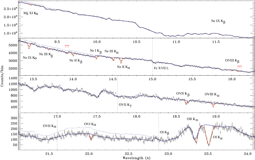
Figure 1.— Co-added MEG spectrum with the best fit continuum (thick blue lines). The dotted lines mark the continuum levels without the Mg, Ne, and O edge absorptions. Red histograms mark the observed absorption lines, and question marks indicate those unidentified ones. The vertical dotted lines mark those undetected lines, which are used to constrain our diagnostic in this work. The bin-size is 10 mÅ.

Figure 2.— Same as the Figure 1, but spectrum is normalized to the best fit continuum.

4. Absorption feature analysis and Results

In this section, we assume that the detected absorption edges and multiple absorption lines are produced in the ISM (see § 5.1 for further discussion) and use them to probe the chemical and thermal properties of the ISM in various phases. In the following course we refer to the neutral and warm ionized ISM as the cool phase, which is traced by the transitions of neutral and mildly ionized ions. To infer the more fundamental properties (e.g., ionic column density $N_{i}$ and the dispersion velocity $v_{b}$) of the intervening gas, we replace the Gaussian profiles with the multiple absline models (§ 2) in modeling the transitions listed in (Table 4). The profile of an absorption line is determined by $N_{i}$ and $v_{b}$ in addition to the three intrinsic parameters $\lambda$, $f_{ij}$, and $\gamma$ (§ 2). Therefore to obtain $N_{i}$ and its error for each ion, we always constrain the $v_{b}$ value as the first step in the following analysis.

4.1. Cool phase interstellar medium

Before discussing the properties of the cool phase of the ISM, we need to revisit the hydrogen properties along the Cyg X-2 sight line. Takei et al. (2002) obtained a total hydrogen column density by assembling the various forms including H I, H II, and H₂ based on the H I 21 cm, H$\alpha$, and CO emission observations, respectively. In their H I estimate, they used the old map of Dickey & Lockman (1990), which offers pointing observations with a grid of $\sim 48^{\prime}$. We here follow their steps but use the Leiden Argentine Bonn (LAB) Galactic H I Survey (Kalberla et al., 2005) that offers a $\sim 30^{\prime}$ spatial grid and 1.3 ${\rm km~{}s^{-1}}$ velocity resolution. To infer the H I column density toward Cyg X-2, we average the column densities from the four adjacent H I observations with respect to their angular separation to Cyg X-2 sight line,

$$N{\rm{}_{CygX2}}=\frac{\sum_{i=1}^{4}N_{i}/d_{i}^{2}}{\sum_{i=1}^{4}1/d_{i}^{2}},$$ (1)

where $N_{i}$ is the column density along each individual sight line, and $d_{i}$ is the angular separation between the sight line and Cyg X-2. Similarly, we define the corresponding uncertainty of this calculation as,

$$\Delta N{\rm{}_{CygX2}}=\frac{\sum_{i=1}^{4}\Delta N_{i}/d_{i}^{2}}{\sum_{i=1}^{4}1/d_{i}^{2}},\ {\rm and}\ \Delta N_{i}=|N_{\rm CygX2}-N_{i}|.$$ (2)

We obtain $N_{\rm CygX2}=1.85\times 10^{21}~{}{\rm cm^{-2}}$ and $\Delta N_{\rm CygX2}=0.05\times 10^{21}~{}{\rm cm^{-2}}$, which is slightly smaller than $2.17\pm 0.20\times 10^{21}~{}{\rm cm^{-2}}$ obtained by Takei et al. (2002).

We use the new filling factor ($f$) for the warm ionized gas to estimate the H II column density. In Takei et al. (2002), the greatest uncertainty of the H II estimate came from the unknown filling factor. By jointly analyzing the H$\alpha$ emission measures and the pulsar dispersion measures toward 157 sight lines, Berkhuijsen et al. (2006) found that the distributions of the warm ionized gas and its filling factor can be characterized as

$$n(z)=n_{0}e^{-z/n_{h}},~{}f(z)=f_{0}e^{z/f_{h}},$$ (3)

with the mid-plane and the scale height values $n_{0}=0.41\pm 0.06~{}{\rm cm^{-3}}$, $f_{0}=0.05\pm 0.01$, $n_{h}=710^{+180}_{-120}$ pc, and $f_{h}=670^{+200}_{-130}$ pc. Along the Cyg X-2 sight line, the H$\alpha$ EM and the H II column density can then be written as

$$EM=\frac{n_{0}^{2}}{\sin b}\int^{\infty}_{0}fe^{-2z/z_{h}}dz$$ (4)

and

$$N_{\rm HII}=\frac{n_{0}}{\sin b}\int_{0}^{D\sin b}fe^{-z/z_{h}}dz,$$ (5)

where $b$ and $D$ are the Galactic latitude and the distance of Cyg X-2, respectively. We explore the allowed parameter spaces of $n_{0}$, $n_{h}$, $f_{0}$, and $f_{h}$ that satisfy the EM toward the Cyg X-2 sight line of $1.28\pm 0.33\times 10^{20}~{}{\rm cm^{-5}}$ (inferred from the H$\alpha$ map after a correction for the extinction; Takei et al. 2002), and then use the allowed values to estimate the H II to $N_{\rm HII}=0.53_{-0.10}^{+0.23}\times 10^{21}~{}{\rm cm^{-2}}$.

Adopting the estimated H₂ value of $<0.10\times 10^{21}~{}{\rm cm^{-2}}$ from Takei et al. (2002), we obtain the total hydrogen. Table 5 compares the various components of hydrogen derived in this work and obtained by the Takei et al..

Table 5Hydrogen column density toward Cyg X-2

	Column Density
	($10^{21}~{}{\rm cm^{-2}}$)
Form	Takei et al.	This work
H I	$2.17\pm 0.20$	$1.85^{+0.05}_{-0.05}$
H II	$0.70\pm 0.18^{a}$	$0.53^{+0.22}_{-0.08}$
H2	$<0.10$	—
total	$2.87^{+0.25}_{-0.23}$	$2.38^{+0.23}_{-0.10}$

Note. — ^a Value derived with the assumed filling factor $f=0.2$ (Takei et al., 2002).

We now measure the neutral column densities of Ne, O, and Mg from their absorption edges. Since the 1s–3p absorption lines of Ne I and Ne II are well separated in the spectrum and the observed neon absorption edge is very close to the Ne I 1s–3p transition (Fig. 1; Tables 3 and 4), it is therefore justified to believe that this edge is solely due to Ne I (see also Juett et al. 2006). Adopting the absorption cross sections from Balucinska-Church & McCammon (1992) (Table 3), we obtain log[N_NeI(cm^-2)] = 17.25(17.18, 17.31) at 90% confidence level. Similarly, we obtain log[N_OI(cm^-2)] = 17.84(17.78, 17.89). For Mg, because of its low ionization energy (7.65 eV; Moore 1970), the Mg II is believed to be the dominant ion in neutral hydrogen region among all charge states (e.g., Savage & Sembach 1996). Therefore the edge measurement in fact yields the Mg II column density, i.e., log[N_MgII(cm^-2)] = 16.92(16.77, 17.02).

We then use the absorption line model, absline (§ 2; Yao & Wang 2005), to infer the column densities ($N_{i}$) of each low ionization ions. For Ne I, the 1s–3p absorption line and the neutral absorption edge in fact trace the same gas. The same is true for O I absorption edge and its 1s–2p and 1s–3p absorption transitions and other ions with multiple transitions (Table 4). To assure the Ne I and O I column densities measured from the edges being consistent with those measured from the lines at 90% confidence levels, we find that $v_{b}$ is allowed to vary between 0 and $75~{}{\rm km~{}s^{-1}}$. We use this velocity range in absline models to infer column densities of all low ionization ions (Table 4). During these measurements, the column density and the $v_{b}$ of a single ion in multiple transitions are linked.

With these column densities, we can infer the chemical abundances of the cool phase ISM. Neon is a noble element and is unlikely to be depleted into dust grains. We then add up the Ne I, Ne II, and Ne III and compare the total with the $N_{H}$. For oxygen, since O I has a very similar ionization energy as H I, the ratio $N_{\rm{OI}}/N_{\rm{HI}}$ thus approximates its abundance in the gas phase. Note that the ratio of $N_{\rm{OI}}/N_{\rm{HI}}$ is inconsistent with that of $N_{\rm{OII}}/N_{\rm{HII}}$. This discrepancy may reflect an either incomplete assessment of the true amount of O II and/or H II, or that the two ratios differ by nature. In the case of the determination of the amount of ionized oxygen, there are a few issues to consider. While the column-density ratio of O II/O I obtained in this work is consistent with that obtained by Juett et al. (2004) in a systematic survey of the complex oxygen absorption edge structure, our search grid does not pick up significant amounts of oxygen in higher ionization stages such as O III as in Juett et al. (2004). Including these amounts would slightly ease the discrepancy. The instrumental resonance at the O II 1s-2p location is generally well determined. On the other hand, any contributions to this resonance that might have been over estimated would actually increase the discrepancy. For magnesium, we simply compare the column density of the dominant ion Mg II to that of the total hydrogen. The abundances of Ne, O, and Mg in the cool ISM phase are reported in Table 6.

Table 6Number ratios of O, Ne, Mg, and Fe to H

	X/H	X/H	X/H	X/H	X/H	X/H
X	($10^{-4}$)	($10^{-4}$)	($10^{-4}$)	($10^{-4}$)	($10^{-4}$)	($10^{-4}$)
Ne	1.23	1.00	0.69	0.87	$0.84^{+0.13}_{-0.10}$	—
O	8.51	5.45	4.57	4.90	$3.83^{+0.48}_{-0.43}$	$5.81^{+1.30}_{-1.34}$
Mg	0.39	0.35	0.34	0.25	$0.35^{+0.09}_{-0.11}$	$0.33^{+0.09}_{-0.09}$
Fe	0.32	0.28	0.28	0.27	$\cdots$	$<0.31$
Ref.	1	2	3	4	5	6

Note. — References.—(1) Anders & Grevesse (1989); (2) Holweger (2001); (3) Asplund et al. (2005); (4) Wilms et al. (2000); (5) Abundances in the cool phase ISM derived in this work (§ 4.1). (6) Abundances in the hot phase ISM derived in this work (§§ 4.2 and 5.4; Table 7).

4.2. Hot phase interstellar medium

As for the low ionization ions, we use multiple absline models to infer column densities of highly ionized ions. Since in the hot ISM, the line broadening is dominated by the non-thermal velocity (e.g., turbulence; Savage et al. 2003; Yao & Wang 2005, 2006), we ignore the subtle thermal velocity difference of different ions and use the same $v_{b}$ value in the absline model for all transitions. In this modeling, we also link the column density of individual ions in multiple transitions (e.g., 1s–2p and 1s–3p of O VIII; Table 4), except for the O VII K$\alpha$ that has not been detected while the O VII K$\beta$ line is significant (see § 5.3 for further discussion). By doing this, we find the $v_{b}$ can be directly constrained as $104^{+43}_{-54}~{}{\rm km~{}s^{-1}}$ although any individual lines are unresolved (§ 3). This constraint comes partly from the ratio of multiple transitions of same ions (e.g., Yao & Wang 2006) and partly from using the same $v_{b}$ in all transitions. The latter is equivalent to co-adding all the detected absorption lines to obtain an S/N ratio of $>200$ per 10-mÅ spectral bin around an absorption line. With the constrained $v_{b}$, we further infer the $N_{i}$ for different ions (Table 4).

We now use $N_{i}$ to probe the thermal and chemical properties of the hot ISM. Since a significant O VII K$\alpha$ line has not been detected, it is not used as a constraint in the following absorption line diagnostics. Neither is O VI used because it likely arises from a different location from the $\sim 10^{6}$ K gas discussed here (see §§ 5.5 and 5.6 for further discussion). If the hot gas is isothermal, then the ratio of $N_{i}$ between the different ionization states of the same ion (e.g., O VII and O VIII) provides a unique probe of its temperature and the equivalent hydrogen column density in the hot phase (e.g., Sutherland & Dopita 1993; Yao & Wang 2005). With the constrained temperature, we can further infer the relative abundances of O/Ne, Mg/Ne, and Fe/Ne by comparing the $N_{i}$ of O VII (or O VIII), Mg XI, and the nondetected Fe XVII to that of Ne IX (Yao & Wang, 2005). We realize this powerful diagnostic by jointly analyzing the multiple high ionization absorption lines step by step, as illustrated in Table 7 (Case I). Note that the above characterization of the hot gas only accounts for $<10\%$ of the observed O VI absorptions.

Table 7Step-by-step absorption line diagnostic of the hot gas properties

Included lines	log[$N{\rm{}_{H}(cm^{-2})}$]	log[$T$(K)]	$\Gamma$	O/Ne	Mg/Ne	Fe/Ne
Case I
O VII, O VIII	$19.39^{+0.09}_{-0.07}$	$6.28^{+0.03}_{-0.02}$	$\cdots$	$\cdots$	$\cdots$	$\cdots$
O VII, O VIII, Ne IX	—	—	$\cdots$	$0.86^{+0.16}_{-0.15}$	$\cdots$	$\cdots$
O VII, O VIII, Ne IX, Mg XI	—	—	$\cdots$	—	$1.08^{+0.26}_{-0.27}$	$\cdots$
O VII, O VIII, Ne IX, Mg XI, Fe XVII	—	—	$\cdots$	—	—	$<1.4$
Case II
O VII, O VIII, Ne VIII, Ne IX, Ne X, Mg XI, Fe XVII	$19.38^{+0.05}_{-0.04}$	$6.31^{+0.14}_{-0.04}$	10(1, 18)	$1.00^{+0.19}_{-0.17}$	$1.23^{+0.29}_{-0.26}$	$<1.23$

Note. — The X/Ne ratio is in units of the solar value of Anders & Grevesse (1989). See text for the detail.

The derived chemical properties are robust against different characterizations of the thermal properties of the hot ISM. The hot gas can extend as far as several kpc from the Galactic plane (§ 1 and references therein), therefore the isothermal assumption adopted above may not be sufficient to describe its thermal properties (e.g., Yao & Wang 2007; Yao et al. 2009). To examine the dependency of the obtained chemical abundances on different approximations to the gas thermal properties, we explore a more complex scenario by assuming that the column density of the hot gas follows a power law function of the gas temperature,

$$N=N_{0}\left(\frac{T}{T_{\rm max}}\right)^{\Gamma}.$$ (6)

Such a characterization can be derived assuming that both the gas density and temperature decrease exponentially as a function of distance away from the Galactic plane (Yao & Wang, 2007; Yao et al., 2009). We then use this distribution to jointly analyze all the highly ionized absorption lines used above at the same time. To obtain a better constraint on the model parameters, we also include in our analysis the nondetection of Ne VIII and Ne X K$\alpha$ transitions. The new constrained O/Ne, Mg/Ne, and Fe/Ne (Case II in Table 7) are consistent with those derived in the isothermal case. This characterization can account for $<45\%$ of the observed O VI absorptions.

5. discussion

5.1. Location of the absorption

The intervening gas that is responsible for the observed absorption features could be either the various phases of the ISM or the circumstellar material associated with the Cyg X-2 system. Since the binary is moving toward the Sun at a velocity of $\sim 220~{}{\rm km~{}s^{-1}}$ (§ 1), the line kinematics are thus the most straightforward way to distinguish these two scenarios. Unfortunately, the accuracy of the current atomic data make such a task very challenging. For example, the newly calculated rest frame wavelength of O VII K$\beta$ is off by $\sim 400~{}{\rm km~{}s^{-1}}$ from the values commonly referenced (Table 1 and references therein). The theoretical values for the low ionization ions are even less reliable, as already demonstrated in Juett et al. (2004, 2006). To select more reliable rest frame wavelengths for high ionization ions, we picked up those values from Table 1 that are consistent within $100~{}{\rm km~{}s^{-1}}$ among different references, which include O VIII, Ne IX, and Mg XI K$\alpha$ and O VIII K$\beta$ transitions. For low ionization ions, we adopted the measured values from Juett et al. (2004, 2006), which include O I, Ne II, and Ne III K$\alpha$ and Ne I–Ne III K$\beta$. We found that velocity shifts of our detected absorption lines are all consistent with the reference “rest frame wavelengths” within $\sim 100~{}{\rm km~{}s^{-1}}$. The statistical uncertainties of the line centroids are usually much smaller due to the high spectral quality (Table 4). On the other hand, if the absorption lines reflect the circumstellar material at different ionization states, they are expected to be Doppler shifted and broadened at velocities comparable to the escape velocity of the system (Yao & Wang, 2005), which is inconsistent with the narrowness of the detected lines (§ 4). Furthermore, the consistent measurements of the Ne IX column density (Fig. 3), for example, indicate a lack of ionization variation that could be expected at different source flux levels in a photoionized scenario. The above arguments suggest that all the absorption features are consistent with an ISM in origin, although the circumstellar scenario with some specific geometric effects cannot be completely ruled out. It is worth noting that highly ionized circumstellar material has indeed been observed via broad emission lines which are consistent with the blueshift implied by the source’s motion towards the Sun (§ 5.3 and Schulz et al. 2009).

Figure 3.— Ne IX absorption lines and the measured column densities at various source flux levels in the four different observations. The bin size is 10 mÅ.

5.2. References to the rest frame wavelengths

If the above detected absorption lines indeed arise from the multiple phases of the ISM, their line centroids are a good reference for the rest frame wavelengths of the corresponding atomic transitions. Although the spectral resolution (the full width at half maximum; FWHM) of the MEG is $\sim$23 mÅ, the centroid of a line can be measured as accurately as one tenth of that (e.g., Ishibashi et al. 2006 and Table 4). In contrast, theoretical calculations, especially for the low ionization ions, are yet to merge (Table 1; Juett et al. 2004, 2006).

There are two main systematic uncertainties that affect the measurement of the line centroids presented in this work. The first comes from the instrumental calibrations. As discussed in § 3, the first step in our data reduction is to determine the zeroth order source position; any uncertainty of the position will be linearly propagated to the whole wavelength scale. This uncertainty affects short wavelengths more than it affects long wavelengths. To quantify this effect, for each of the four observations (Table 2), we compare the positive and the negative arms in measuring the O I K$\alpha$ line, the longest wavelength line of our interest (Table 4). We find that except for the short observation (ObsID 1016) in which there is not enough counts near the line, the difference in the other three individual observations is less than 6.6 mÅ. Since we measured the averaged value of the two arms in our final data analysis, we then take the systematic error due to the calibration to be $<4.7$ ($=6.6/\sqrt{3-1}$) mÅ.

The other source of the systematic bias is due to the differential rotation of the ISM toward the Cyg X-2 sight line. Gas in the Galactic disk at different radii is rotating at different velocities around the Galactic center (GC) in near circular orbits; gas close to the GC has a shorter period than that further out. For gas at radius $R$ and with a rotational velocity $V$ moves with respect to the local standard rest frame (LSR) at a speed of

$$V_{r}=R_{0}\sin l\left(\frac{V}{R}-\frac{V_{0}}{R_{0}}\right),$$ (7)

where $R_{0}$ and $V_{0}$ are the radius of the LSR and its rotation velocity, respectively (Sparke & Gallagher, 2000). The observed differential velocity is then the integral of all $R$s and $V$s along the pathlength to Cyg X-2.

The velocity shift due to the differential rotation is very small. For low ionization ions, this effect can be revealed from the 21 cm H I emission. Averaging the velocities with respect to the column densities for the four adjacent H I observations around the Cyg X-2 sight line (§ 4.1), we obtain $\overline{V_{r}}=-8~{}{\rm km~{}s^{-1}}$. For high ionization ions, since they extend to a much larger scale than the low ionization ones (§ 1), the “halo-lagging” effect (e.g., Rand 1997, 2000) must be taken into account. We here assume that, (1) the density of the hot gas decreases exponentially along the vertical distance away from the Galactic plane with a scale height of 3 kpc (e.g., Bowen et al. 2008; Yao et al. 2008); (2) the rotation velocity linearly decreases from $V_{0}$ and $V$ at the Galactic plane to zero at a height $z_{0}$ above the Galactic plane; and (3) the velocity at radii between $R_{0}$ and $R$ can be linearly interpolated from $V_{0}$ and $V$. For the LSR, we take $R_{0}=8$ kpc and $V_{0}=220~{}{\rm km~{}s^{-1}}$, and for the Galactic radius of Cyg X-2, $R=11$ kpc. Again, we average the $V_{r}$ with respect to the column density along the line of sight. For an extreme case, $z_{0}$ = 1.5 kpc (where Cyg X-2 is located; § 1), we obtain an firm upper limit of $\overline{V_{r}}<117~{}{\rm km~{}s^{-1}}$ by taking $V=164~{}{\rm km~{}s^{-1}}$ that represents the smallest velocity derived from the smallest H I emission velocity of $V_{r}=-100~{}{\rm km~{}s^{-1}}$ along the Cyg X-2 sight line (§ 4.1). If assuming a more reasonable $z_{0}$ = 8 kpc, we then obtain $\overline{V_{r}}\sim 56~{}{\rm km~{}s^{-1}}$, which corresponds to an uncertainty of 4.4, 4.1, and 1.7 mÅ at wavelength of 23.5, 22, and 9 Å, respectively.

It is worth pointing out that besides the absorption lines presented in this work, the highly ionized emission lines observed in stellar coronae (e.g., Huenemoerder et al. 2003) also provide complementary references for the rest frame wavelengths of the atomic transitions. The wavelengths measured in this work are remarkably consistent with those detected in stellar coronae.

For transitions of the low ionization ions, the absorption line centroids and the edge wavelengths reported in Juett et al. (2004, 2006), though with larger statistical errors due to the lower counting statistics in their used spectra, are consistent with the values obtained in this work.

5.3. Mystery of the un-detected O VII K$\alpha$ line at 21.6 Å

In our high quality spectrum, we did not detect the O VII K$\alpha$ absorption line, which however, is expected to be one of the most prominent lines because of the high abundance of oxygen, the high ionization fraction of O VII in a broad temperature range (Sutherland & Dopita, 1993), and the large absorption oscillation strength of the transition (Table 1). Figure 4 exhibits the expected O VII K$\alpha$ absorption based on the measurement of the detected O VII K$\beta$ and non-detected O VII K$\gamma$ lines (Table 4).

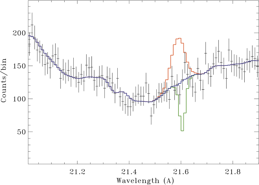
Figure 4.— Observed spectrum, the best fit continuum (blue), and the predicted O VII K$\alpha$ line absorptions (green) from the observed O VII K$\beta$ transition (Table 4). The red line marks the O VII resonance emission needed to fill in the O VII K$\alpha$ absorption.

The absence of the O VII K$\alpha$ absorption is puzzling. One obvious possibility would be that there is an O VII resonance emission line with a flux compensating for the line absorption. If this is the case, it requires a line flux of $4.9\times 10^{-4}~{}{\rm photons~{}s^{-1}~{}cm^{-2}}$. Emission lines tracing the photoionized accretion-disk-corona (ADC) have been observed in this source, but the lines are generally very broad with a minimum FWHM of $\sim 800~{}{\rm km~{}s^{-1}}$ (Schulz et al., 2009). Figure 4 demonstrates such a local broad emission line at the systematic velocity of Cyg X-2 ($-220~{}{\rm km~{}s^{-1}}$; § 1) on top of the continuum; its flux is scaled to that of the missing O VII K$\alpha$ at the corresponding wavelength. Although such a line has the power to compensate for the absorption, the slight offset as well as the stark difference in line broadening has to leave a significant residual with respect to the line absorption. The ADC region is also expected to have a very high density, and the intercombination line usually dominates the triplet emission for the He-like ions (Schulz et al., 2009). If it is the intercombination rather than the resonance transition that fills in the absorption, besides its broadening, it is also expected to be blue-shifted at $\sim 2.7\times 10^{3}~{}{\rm km~{}s^{-1}}$ for O VII. Such a velocity shift was not observed in other detected emission lines (Schulz et al., 2009). Also, the intercombination line will be slightly broader than the resonance and should leave a similar residual. The ionization parameters derived from the emission lines are also too high to expect the emission from the oxygen ions (Schulz et al., 2009). Another source that could fill the expected O VII K$\alpha$ line absorption is the scattered resonance line emission of the hot ISM. But this diffuse emission presumably uniformly fills the Chandra field of view, and thus would only produce a very broad rather than a narrow emission enhancement in the grating spectrum. Futhermore, the intinsic O VII intensity of the diffuse ISM along the Cyg X-2 sight line is expected to be $\sim 2.2-6.4$ ${\rm photons~{}s^{-1}~{}cm^{-2}~{}str^{-1}}$ (Yoshino et al., 2009), and the foreground cool ISM will attenuate this emission to be $\sim 0.3-0.9~{}{\rm photons~{}s^{-1}~{}cm^{-2}~{}str^{-1}}$ (taking $N_{\rm H}=2.38\times 10^{21}~{}{\rm cm^{-2}}$; Table 5) before the emission reaches detectors. The small field of view ($8.3^{\prime}\times 16.6^{\prime}$, the full field of view of two ACIS chips) of Chandra thus could only yield a line flux of $0.03-0.1\times 10^{-4}~{}{\rm photons~{}s^{-1}~{}cm^{-2}}$ at most, which is much less than the missing amount. The consistent measurement of the non-detected O VII K$\alpha$ line between positive and negative grating spetral orders also rules out any possible instrumental effects (e.g., an unfortunate set of hot pixels or unrecognized non-X-ray events precisely at the position of the absorption line on the detector) that could fill the absorption line.

The other detected absorption lines do not seem to be significantly diluted by any peculiar line emission. The putative ADC emission is not expected to affect our absorption measurements in general. The detected ISM lines are nearly unresolved (§ 4), and their measurements rely on the local continuum in a very narrow wavelength range. The generally very broad emission lines as observed in the Cyg X-2 binary system can therefore be regarded as continuum and thus will not generate any confusion to the measurements presented in this work. The only concern with respect to our measurements is a likelihood of the similar peculiar narrow emission lines as may possibly occur in the case of O VII K$\alpha$. For the H- and He-like oxygen and neon ions, the emissivity ratios between the 1s–2p and the 1s–3p transitions in the temperature range of $10^{5}-10^{7}$ K are always larger than the ratios of the corresponding absorption oscillation strengths. Therefore any existing emission will fill more rapidly the 1s–2p lines than the 1s–3p ones. We re-fit the individual K$\alpha$ and K$\beta$ absorption lines of O VIII and Ne IX, and find that the column densities derived from the different transitions are consistent within 1$\sigma$ for each ion. In contrast, the 1s–3p of O VII provides a very tight constraint on O VII column density while the 1s–2p only yields an upper limit (Table 4). This consistent measurement in O VIII and Ne IX could only be incidentally reached when the filled-up portions of the lines were proportional to their absorption oscillation strengths plus the saturation effects. We thus speculate that the chance for the existence of the peculiar emission lines for other ions is small. Limited by the scope of this work, we prefer to leave the mystery of the missing O VII K$\alpha$ absorption line unexplained, and assume that other O VII transitions (e.g., K$\beta$ and K$\gamma$) still faithfully reflect the O VII absorption column in the following sections.

5.4. Chemical abundances in different phases

The chemical abundances of the cool phase ISM presented in Table 6 represent so far the best measurements of the absolute abundances in X-ray. For a comparison, Table 6 also lists several references for the solar/ISM abundances commonly used in the literature. In these references, neon is the one of the most uncertain abundances because its value is usually scaled with respect to other relatively well-studied ones like oxygen, due to the lack of suitable spectral lines in modeling the Sun’s photosphere (e.g., Wilms et al. 2000; Asplund et al. 2005). In contrast, because the total hydrogen column density of the cool phase along the Cyg X-2 sight line is available, the measured neon value in this work offers a valuable reference for its abundance in the ISM. Our measured oxygen abundance is systematically lower than all the referenced values, indicating an oxygen depletion into dust grains (see below), whereas the magnesium value suggests a mild or no depletion (Table 6).

For the hot phase ISM, since the hydrogen is expected to be fully ionized at temperatures $\sim 10^{6}$ K, there is no usable atomic transition to measure its column density. However, assuming that the neon abundance remains the same in both cool and hot phases, we can utilize the established neon abundance in the cool phase to derive the absolute abundances of oxygen, magnesium, and iron in the hot phase based on their measured relative abundances (§ 4.2; Tables 6 and 7).

It is interesting to compare the abundance difference between the cool and hot phases (Table 6). The oxygen abundance in the hot phase is remarkably lower than the old solar value of Anders & Grevesse (1989), but is consistent with the recently revised solar value (Asplund et al., 2005) and the expected value in the ISM (Wilms et al., 2000). However, it is apparently higher than that in the cool phase, which indicates dust grain sputtering and/or recent metal enrichment of the hot phase. If the dust grains were totally destroyed in the hot phase, the difference indicates that $\sim$30% of the total oxygen is likely depleted into dust grains in the cool phase. The consistent measurement of the magnesium abundance in both phases further confirms that very little or no magnesium is depleted into dust grains.

If $\sim 30\%$ ($N_{\rm O}=4.15\times 10^{17}~{}{\rm cm^{-2}}$) of oxgyen is indeed depleted into dust grains, its 1s–2p transition that is analog to that of the atomic form at 23.51 Å would also imprint a significant absorption feature near the position of the instrumental oxide resonance at 23.35 Å. However, visual inspectation does not reveal any absorption line other than the one at 23.35 Å between 22.81 Å (the atomic oxygen edge position) and 23.51 Å (Fig. 1). Several previous works actually attributed the absorption feature at 23.35 Å to oxygen in compound forms rather than to its atomic O II 1s–2p transition (e.g., Paerels et al. 2001; Takei et al. 2002). However, such a attribution would further exacerbate the already deficit of the O II column density (§ 4.1). One possible explanation is that the 1s–2p transition of oxygen in dust grains is completely suppressed due to the effectively filled L (n=2) shell and/or that the transition oscillation strength ($f_{\rm 12}$) for oxygen in compound forms is so small ($<0.05$) that the absorption feature is too weak to be visible.

Let us compare these results with several previous works.

Takei et al. (2002) analyzed the Chandra LETG observation of Cyg X-2 (Table 2) and measured the O I and Ne II 1s–2p transitions and O and Ne absorption edges, but they attributed other features in O K edge complex to compound features rather than to the atomic transitions (e.g., O II and O III lines; see Paerels et al. 2001; Juett et al. 2004). They also used multiple edge models to approximate the complex oxygen absorption edges due to the different compound compositions and different ionization states. Interestingly, their overall measurements and derived oxygen and neon abundances in the cool phases are consistent with ours though with larger statistical errors.

Juett et al. (2004, 2006) systematically investigated the complex structures of the oxygen and neon absorption edges, and they also used a subset (ObsID 1102) of the data analyzed in this work (Table 2). Along the Cyg X-2 sight line, the optical depth of the neon edge they obtained is consistent with that we measured in this work, but their oxygen value is apparently higher. By examining the putative absorption features due to various compounds, they concluded that their data allow 10%-40% of the oxygen to be depleted into dust grains, which is consistent with what we find above through comparing the O/Ne in cool and hot phases.

Yao & Wang (2006) analyzed the multiple absorption lines in a Chandra spectrum of 4U 1820–303 in great detail and found that while about 50% of the oxygen is depleted into dust grains in the cool phase, there is no evidence showing the oxygen depletion in the hot phase, which in general agrees with what we find here. Yao et al. (2006) further detected the Fe XVII absorption line in the Chandra spectrum and concluded that a bulk of the heavily depleted iron in the cool ISM as evidenced in both Far-UV and X-ray wavelength bands (e.g., Savage & Sembach 1996; Juett et al. 2006) has been liberated during the dust sputtering process in the hot phase. However, in this work, we did not detect the Fe XVII line and only obtained an upper limit to the iron column density (Table 4), which prevents us from constraining a meaningful iron abundance (Tables 6 and 7) and further testing the iron depletion and dust grain destruction concluded in Yao & Wang (2006).

The small depletion of magnesium in the cool phase indicated in this work contradicts the heavy ($\lower 2.0pt\hbox{$\,\buildrel\scriptstyle>\over{\scriptstyle\sim}\,$}70\%$) depletion previously concluded based on the measurement of the far-UV Mg II absorption lines in spectra of high latitude stars (e.g., Savage & Sembach 1996 and references therein). This discrepancy could be easily reconciled if a smaller absorption oscillation strength ($f_{ij}$) is applied to these Mg II absorption lines.

5.5. Limit to the large-scale Galactic Halo

The detection of the high ionization absorption lines along the Cyg X-2 sight line has implications for our understanding of galaxy formation and evolution. Highly ionized absorption lines (O VII K$\alpha$ line in particular) have been commonly observed toward extragalactic sources (e.g., Fang et al. 2006; Bregman & Lloyd-Davies 2007). The absorptions could arise from either the large-scale ($>20$ kpc) Galactic halo gas or the hot gas in the extended Galactic disk or a combination of both. The existence of the Galactic gaseous halo has been predicted in many semi-analytic calculations and numerical simulations of disk galaxy formation. The gas, originally accreted from the intergalactic medium, could have been shock-heated to the virial temperature during its in-falling into the dark matter halo’s potential well (e.g., Birnboim & Dekel 2003) and is believed to contain the total baryonic mass comparable to or even greater than the total baryonic matter of stars and the ISM (e.g., Sommer-Larsen 2006). On the other hand, there is mounting evidence showing the existence of the hot gas around the disk galaxies, for instance, the diffuse X-ray emission detected in disk galaxies (e.g., Tüllmann et al. 2006), the spatial distribution of the far-UV O VI absorption and emission (e.g., Savage et al. 2003; Dixon & Sankrit 2008), and the O VII and Ne IX absorptions detected toward the Galactic sources (e.g., Yao & Wang 2005; Juett et al. 2006; this work). Both the morphology and the intensity of the diffuse X-ray emission in the extragalactic sources suggest that the hot gas traces the stellar feedback in the galactic disk (e.g., Tüllmann et al. 2006). The question is, how much the disk hot gas contributes to the total X-ray absorptions observed in the extragalactic sources. Rasmussen et al. (2003) combined the absorption lines detected along three AGN (Mrk 421, 3C 273, and PKS 2155-304) sight lines with the O VII emission measurement from the sounding rocket experiment (McCammon et al., 2002) and estimated a scale length of the absorbing/emitting gas to be $>140$ kpc. In contrast, Yao & Wang (2007) extensively analyzed the absorption lines observed along the Mrk 421 sight line and concluded that the absorbing gas is of a nonisothermal nature and is consistent with a location of several kpc around the Galactic plane. The latter authors further argued that the discrepancy between their results and those obtained by Rasmussen et al. (2003) could be easily reconciled if the metallicity, density distribution, and nonisothermality of the absorbing/emitting gas were considered.

A more direct estimate of the Galactic disk contribution is to compare absorption lines observed toward Galactic sources with those observed toward extragalactic sources. Yao et al. (2008) recently conducted such a differential study by comparing the highly ionized X-ray absorption lines observed towards three sight lines, a distant quasar Mrk 421, LMC X-3 at a distance of $\sim 50$ kpc in the Large Magellanic Cloud, and a Galactic sight line 4U 1957+11, and concluded that all X-ray absorptions toward the extragalactic sources can be attributed to the Galactic disk hot gas.

A major uncertainty of the differential comparison performed by Yao et al. (2008) is the possible non-homogeneity of the disk hot gas. Apparent variation of the X-ray absorptions has been detected along different AGN sight lines (e.g., Bregman & Lloyd-Davies 2007), which however, may not reflect the disk hot gas variation on a global scale because nearly all the observed absorption enhancements are due to the known additional absorption components (e.g., the north polar spur, the Galactic bulge region, etc.). Both far-UV O VI absorption and emission could vary at an angular scale as small as $25^{\prime}$ (Howk et al., 2002; Dixon et al., 2006). For a gas in the CIE state, the population of O VI peaks at intermediate temperatures at which the hot gas cools very efficiently; a bulk of the observed O VI is believed to exist at interfaces of the cool and hot gases (e.g., Savage & Lehner 2006). The O VI thus traces more directly to the embedded cool gas clouds rather than to the hot gas itself. The smooth distributions of the diffuse soft X-ray emission intensity in our Galaxy (again, except for the known emission enhancement regions like the north polar spur, the Galactic center, the Cygnus loop, etc.; Snowden et al. 1997) and around the extragalactic disk galaxies (Tüllmann et al., 2006) in fact suggest that the galactic disk gas is likely to be homogeneous in general.

We now compare the highly ionized absorption lines between the Cyg X-2 sight line and the extragalactic sight line Mrk 421. The latter presents to date the best constrained highly ionized absorptions toward extragalactic sight lines (e.g., Yao & Wang 2007). With respect to the Galactic X-ray binary 4U 1957+11 (Galactic coordinates $l,b=51\fdg 31,-9\fdg 33$) used in Yao et al. (2008), Cyg X-2 is located further away from the Galactic center region and thus the observed absorption should be less affected by the Galactic bulge gas. We jointly analyze the absorption lines toward these two sources by assuming the common disk hot gas has the same thermal properties. We normalize the absorption toward the Cyg X-2 sight line to that toward the Mrk 421 direction by assuming that the absorbing gas is slab-like distributed (e.g., by multiplying a factor of $\sin b$), and obtain the “net” absorption beyond the Cyg X-2 as $\log N{\rm{}_{OVII}(cm^{-2})}=15.56(15.45,15.64)$, and $\log N{\rm{}_{OVII}(cm^{-2})}=15.43(15.27,15.55)$, i.e., the pathlength of Cyg X-2 can account for $\sim 40\%$ of the total absorption toward Mrk 421 sight line. If we further consider the location of Cyg X-2 and assume that its pathlength only samples $<54\%$ of the disk hot gas in the vertical direction (taking its distance of $<12$ kpc and an exponential scale height of 3 kpc; § 1 and Yao et al. 2009), we find that all the X-ray absorption toward the Mrk 421 can be attributed to the Galactic disk hot gas, and obtain upper limits to the “net” absorption beyond the disk as $\log N{\rm{}_{OVII}(cm^{-2})}<15.32$ and $\log N{\rm{}_{OVIII}(cm^{-2})}<15.32$ (Fig. 5). This is consistent with the limits derived by Yao et al. (2008).

Figure 5.— O VII K$\beta$, O VIII K$\alpha$, and O VII K$\alpha$ absorption lines observed in the spectrum of Mrk 421 (cross), overlayed with the best fit continuum (green). The red histograms mark the amount of the absorptions observed toward Cyg X-2 sight line after the correction for the Galactic latitude dependence. The blue histograms indicate the total expected Galactic disk absorptions by scaling the observed absorptions along the Cyg X-2 pathlength with an exponential scale height of 3 kpc. See text for the detail.

5.6. Predicted far-UV absorption and emission

A large amount of far-UV absorption and emission is expected to arise from the observed O VI-bearing gas. The detected O VI along the Cyg X-2 sight line ($\log N{\rm{}_{OVI}[cm^{-2}]}=15.73^{+0.17}_{-0.13}$; Table 4) is the largest O VI column density observed so far. If assuming the solar abundance ratios of N/O and C/O, we can estimate the expected N V and C IV column densities (and thus the corresponding EWs of their L transition lines) associated with the O VI-bearing gas for the isothermal assumption (§ 4.2). Unlike the LMC X-3 sight line toward which the hot O VII-bearing gas can explain all the observed O VI absorptions (Yao et al., 2009), the hot ($T\sim 10^{6}$ K) gas toward the Cyg X-2 sight line accounts for only a tiny portion of the observed O VI (§ 4.2), leaving much of the O VI to arise from the conductive interfaces (e.g., Slavin 1989; Savage & Lehner 2006). Dixon et al. (2006) recently derived an electron density of $n_{e}=0.29~{}{\rm cm^{-3}}$ at the interfaces by comparing the O VI emission and absorption along the same sight line. If taking this density and also assuming the solar abundance ratios, we can estimate the expected O VI, N V, and C IV emission line intensities from the interfaces. Note that if assuming 55% (§ 4.2) of the observed O VI arise from the interfaces, the adopted electron density yields an O VI-gas size of 34 pc or a filling factor of 4% for O VI at its peak ionization fraction. Figure 6 shows the expected N V and C IV column densities and the predicted intrinsic and attenuated line intensities by taking the reddening $E(b-V)=0.4$ (McClintock et al., 1984) and the extinction from Fitzpatrick (1999). These absorption and emission lines, N V and C IV in particular, are measurable and thus can be tested with the Cosmic Origins Spectrograph (COS) and the Space Telescope Imaging Spectrograph (STIS) installed on Hubble Space Telescope (HST) with reasonably long exposures.

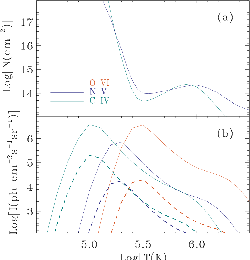
Figure 6.— (a) Detected O VI and expected N V and C IV column densities as a function of temperature. (b) Predicted doublet line emission intensity for He-like ions O VI, N V, and C IV as a function of temperature. The dotted lines are the attenuated intensities assuming all emission arising behind dust grains.

6. Summary

We presented a high resolution X-ray spectroscopy study of the multiphase interstellar medium based on four observations of Cyg X-2 with the Chandra High Energy Transmission Grating Spectrometer. Our main results and conclusion can be summarized as follows:

1. We measure the properties of 14 identified absorption lines and 3 absorption edges in the final co-added spectrum. Modeling these lines and edges we obtain the column densities of O I-O II, Ne I-Ne III, O VI-O VIII, Ne IX, and Mg XI.

2. We demonstrate that these absorption features trace the various phases of the interstellar medium rather than circumstellar material dynamically associated with the Cyg X-2 system. The well constrained centroids of the absorption features provide a good reference for the rest frame wavelengths of the corresponding atomic transitions.

3. Comparison between absorption edges and absroption lines of Ne I and O I constrains velocity dispersion in cool phase ISM to be $v_{\rm b}<75~{}{\rm km~{}s^{-1}}$, and joint analysis of multiple high ionization absorption lines (O VI-O VIII, Ne IX, and Mg XI) yields $v_{\rm b}$ in hot phase ISM to be $104_{-54}^{+43}~{}{\rm km~{}s^{-1}}$.

4. Complementing the absorption data with H I 21 cm, H$\alpha$, and CO emission data, we derive absolute abundances of neon, oxygen, and magnesium in the cool phase ISM to $0.89^{+0.13}_{-0.11}\times 10^{-4}$, $3.83^{+0.48}_{-0.43}\times 10^{-4}$, and $0.35^{+0.09}_{-0.11}\times 10^{-4}$, respectively. By jointly analyzing the multiple high ionized absorption lines we also derive the abundances of oxygen and magnesium in the hot phase as $5.30^{+1.18}_{-1.33}\times 10^{-4}$ and $0.31^{+0.08}_{-0.09}\times 10^{-4}$, which are robust against different assumed temperature distributions of the absorbing gas. In the cool phase, while about 30% of the oxygen is depleted into dust grains, there is no evidence for magnesium depletion.

5. The observed O VII and O VIII absorptions toward Cyg X-2 can already account for $\sim 40\%$ of the high ionization absorptions observed toward the Mrk 421 sight line. By considering the location of Cyg X-2 and the spatial distribution of the Galactic hot gas, this means that all the high ionization absorptions observed toward the extragalactic sight line can be attributed to the extended Galactic disk.

6. A large amount of far-UV absorption and emission is expected to arise from the O VI-bearing gas. The expected N V and C IV column densities and the predicted emission line intensites are measurable with the COS and STIS aboard HST.

References

- Anders & Grevesse (1989) Anders, E., & Grevesse, N. 1989, Geochim. Cosmochim. Acta, 53, 197
- Asplund et al. (2005) Asplund, M., Grevesse, N., & Sauval, J., 2005, ASPC, 336, 25
- Balucinska-Church & McCammon (1992) Balucinska-Church, M., & McCammon, D. 1992, ApJ, 400, 699
- Barrus et al. (1979) Barrus, D. M., et al. 1979, PhRvA, 20, 1045
- Behar & Netzer (2002) Behar, E., & Netzer, H. 2002, ApJ, 570, 165
- Berkhuijsen et al. (2006) Berkhuijsen, E. M., Mitra, D., & Müller, P. 2006, Astron. Nachr., 327, 82
- Birnboim & Dekel (2003) Birnboim, Y, & Dekel, A. 2003, MNRAS, 345, 349
- Bowen et al. (2008) Bowen, D. V., et al. 2008, ApJS, in press
- Bregman & Lloyd-Davies (2007) Bregman, J. N., & Lloyd-Davies, E. J. 2007, ApJ, 669, 990
- Canizares et al. (2005) can05 Canizares, C. R., et al. 2005, SPIE, 597, 253
- Casares et al. (1998) Casares, J., Charles, P., & Kuulkers, E. 1998, ApJ, 493, L39.
- Cowley et al. (1979) Cowley, A. P., Crampton, D., & Hutchings, J. B. 1979, ApJ, 231, 539
- Dickey & Lockman (1990) Dickey, J. M., & Lockman, F. J. ARA&A, 28, 215
- Dixon et al. (2006) Dixon, W. V. D., Sankrit, R., & Otte, B. 2006, ApJ, 647, 328
- Dixon & Sankrit (2008) Dixon, W. V. D., & Sankrit, R. 2008, ApJ, in press
- Fang et al. (2006) Fang, T., et al. 2006, ApJ, 644, 174
- Ferrière (2001) Ferrière, K. 2001, Rev. Mod. Phys., 73, 1031
- Fitzpatrick (1999) Fitzpatrick, E. L. 1999, PASP, 111, 63
- García et al. (2005) García, J., et al. 2005, ApJ, 158, 68
- Gorczyca (2000) Gorczyca, T. W. 2000, Phys. Rev. A., 61, 024702
- Gorczyca & McLaughlin (2005) Gorczyca, T. W., & McLaughlin, B. M. 2005, Bull. Am. Phys. Soc., 50, 39
- Gu (2003) Gu, M. F. 2003, ApJ, 582, 1241
- Holweger (2001) Holweger, H. 2001, AIPC, 598, 23
- Howk et al. (2002) Howk, J. C., et al. 2002, ApJ, 572, 264
- Huenemoerder et al. (2003) Huenemoerder, D. P., Canizares, C. R., Drake, J. J., & Sanz-Forcada, J. 2003, ApJ, 595, 1131
- Ishibashi et al. (2006) Ishibashi, K, et al. 2006, ApJ, 644, L1171
- Juett et al. (2004) Juett, A., et al. 2004, ApJ, 612, 308
- Juett et al. (2006) Juett, A., et al. 2006, ApJ, 648, 1066
- Kalberla et al. (2005) Kalberla, P. M. W., et al. 2005, A&A, 440, 775
- Kallman et al. (2004) Kallman, T. R., et al. 2004, ApJS, 155, 675
- Lockman et al. (1986) Lockman, F. J., Hobbs, L. M., & Shull, J. M. 1986, ApJ, 301, 380
- McKee & Ostriker (1977) McKee, C. F., & Ostriker, J. P. 1977, ApJ, 218, 148
- McCammon et al. (2002) McCammon, D., Almy, R., Apodaca, E., et al. 2002, ApJ, 576, 188
- McClintock et al. (1984) McClintock, J. E., et al. 1984, ApJ, 283, 794
- Morton (1991) Morton, D. C. 1991, ApJS, 77, 119
- Morton (2003) Morton, D. C. 2003, ApJS, 149, 205
- Moore (1970) Moore, C. E. 1970, Ionization Potentials and Ionization Limits Derived from the Analysis of Optical Spectra (NSRDS-NBS Rep. 34; Washington, DC:NBS)
- Orosz & Kuulkers (1999) Orosz, J. A., & Kuulkers, E. 1999, MNRAS, 305, 132
- Overbeck (1965) Oberbeck, J. W. 1965, ApJ, 141, 864
- Paerels & Kahn (2003) Paerels, F. B. S., & Kahn, S. M. 2003, ARA&A, 41, 291
- Paerels et al. (2001) Paerels, F. B. S., et al. 2001, ApJ, 546, 338
- Page et al. (2003) Page, M. J., et al. 2003, MNRAS, 345, 639
- Predehl & Klose (1996) Predehl, P., & Klose, S. 1996, A&A, 306, 283
- Predehl et al. (2000) Predehl, P., et al. 2000, A&A, 357L, 25
- Rand (1997) Rand, R. J. 1997, ApJ, 474, 129
- Rand (2000) Rand, R. J. 2000, ApJ, 537, L13
- Rasmussen et al. (2003) Rasmussen, A., Kahn, S. M., & Paerels, F. 2003, in The IGM/Galaxy Connection: The Distribution of Baryons at z=0, ed. J. L. Rosenberg & M. E. Putman (ASSL Conf. Proc. 281; Dordrecht: Kluwer), 109
- Rybicki & Lightman (1979) Rybicki, G. B., & Lightman, A. P. 1979, Radiative Processes in Astrophysics (New York: Wiley)
- Savage et al. (1990) Savage, B. D., Edgar, R. J., & Diplas, A. 1990, ApJ, 361, 107
- Savage & Sembach (1996) Savage, B. D., & Sembach, K. R. 1996, ARA&A, 34, 279
- Savage et al. (2003) Savage, B. D., et al. 2003, ApJS, 146, 125
- Savage & Lehner (2006) Savage, B. D., & Lehner, N. 2006, ApJS, 162, 134