Equilibrium and nonequilibrium effects in the collapse of a model polypeptide

Abstract

We present results of molecular simulations of a model protein whose hydrophobic collapse proceeds as a cascade of downhill transitions between distinct intermediate states. Different intermediates are stabilized by means of appropriate harmonic constraints, allowing explicit calculation of the equilibrium free energy landscape. Nonequilibrium collapse trajectories are simulated independently and compared to diffusion on the calculated free energy surface. We find that collapse generally adheres to this surface, but quantitative agreement is complicated by nonequilibrium effects and by dependence of the diffusion coefficient on position on the surface.

In Kramers theory a chemical reaction is modeled by Brownian motion of a particle in an effective field of force Kramers (1940). The force is related to the change in the free energy of the system as it moves along a reaction coordinate that parameterizes the physical or chemical transformation involved. The rate of the reaction is then determined by the shape of the (free) energy landscape and by an effective diffusion constant. In recent research the energy landscape has been frequently invoked in discussions of complex biological phenomena, such as folding of proteins and RNA Fun ; Dil ; RNA . Furthermore, the energy landscape has been measured experimentally for some biophysical systems Lan , where it is assumed that a single reaction coordinate captures a process which occurs in a high dimensional phase space. In the case of two-state protein folding, theoretical studies have indicated that effective diffusion along a reaction coordinate is described by the value of the diffusion coefficient which is not constant, as in Kramers theory, but coordinate-dependent Chahine et al. (2007); Best and Hummer (2006). Such dependence of diffusion on the position on the free energy surface will be even more important for downhill protein folding which occurs in the absence of a free energy barrier and is, therefore, a diffusion-limited process.

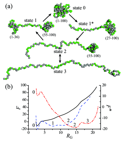
Figure 1: (a) Polymer conformations corresponding to different states. H-monomers are grey (dark), P-monomers are green (light). Numbers in brackets indicate monomers comprising compact globules. (b) Free energies $F$ and $F^{*}$ for the impeding force $f_{0}=0$ (solid) and $f_{0}=0.02\varepsilon/\sigma$ (dash), $0.04\varepsilon/\sigma$ (dash-dot). $F$, $F^{*}$ are given in the units of $k_{\rm B}T$ and $R_{\rm G}$ in the units of $\sigma$. The dashed-dotted line is shifted up by $40k_{\rm B}T$.

In this letter we study thermodynamics and kinetics of polymer hydrophobic collapse as a basic model for downhill protein folding. We find that effective diffusion slows down by an order of magnitude when the polymer enters the free energy basin of its collapsed (ground) state, so that subsequent diffusion across this narrow region of the phase space takes an appreciable fraction of the overall collapse time. In the absence of a free energy barrier, the application of the diffusive model to protein folding requires an accurate knowledge of the entire ground state basin, which cannot be deduced from irreversible folding trajectories alone. Below we describe an efficient and accurate method for the calculation of multi-dimensional free energy surfaces, including high gradient slopes of the ground state basin. The method is based on subjecting a polymer to a set of harmonic constraints and thereby preventing its collapse to the ground state. Comparing the results of simulations of an unconstrained polymer and of the polymer harmonically bound to various positions on the free energy surface, we conclude that the freely collapsing polymer fails to achieve local equilibrium as it enters the ground state basin. Furthermore, for the specific polymer considered here, a local nonequlibrium effect is observed at the entrance to the basin, which is caused by a relatively intense collision of different parts of the polymer. Such nonequilibrium effects are beyond the scope of the Kramers model and its use may introduce artifacts in the numerical analysis of experimentally observed folding times. It remains an open question how the Kramers theory can be modified to account for both local and more general nonequilibrium effects. However, in computational studies as described here, combined simulations of irreversible folding trajectories and of harmonically constrained macromolecules can provide detailed information on their equilibrium free energies as well as indicate various nonequilibrium effects.

We consider a simple HP model of a protein, consisting of a polymer chain of “hydrophobic” (H) and “hydrophilic” (P) spherical monomers. HH interactions are modeled by the attractive Lennard-Jones potential, $u_{\rm LJ}(r)=4\varepsilon[(\sigma/r)^{12}-(\sigma/r)^{6}]$, where $\varepsilon=5k_{\rm B}T/3$ and $\sigma$ is the monomer diameter. HP and PP interactions are modeled by the repulsive part of the same potential. The fraction of P-residues in a sequence is chosen to be equal to the fraction of monomers on the surface of a compact spherical globule. This criterion yields 44 P-residues for a chain of length 100 End (a). The data presented below are for the particular sequence HPHHHPPPPHPHPHHHPPHHPPHHPPHHPHHHPHHHPPPHPHPHPPPPHPHPPPHHHPHPPHHHHHHHHPHPPHPPHPHHPHHPPHHPHHHHHPHHPPHH, that has been generated randomly to satisfy this condition End (b). The polymer bond length $a$ and the angle between adjacent bonds $\phi$ are constrained by means of the FENE Grest and Kremer (1986) and harmonic potentials, respectively: $u_{\rm F}(a)/k_{\rm B}T=-33.75\ln[1-(2a/3\sigma)^{2}]$ and $u_{\rm H}(\phi)/k_{\rm B}T=50(\phi-2\pi/3)^{2}$. The polymer dynamics are simulated by solving the Langevin equation for individual monomers $i$, $m\ddot{\bm{r}}_{i}=-\gamma\dot{\bm{r}}_{i}+\bm{F}_{i}+\bm{R}_{i}$, where $m$ is the monomer mass, $\gamma$ is the drag coefficient, $\bm{F}_{i}$ is the conservative force, and $\bm{R}_{i}$ is the Gaussian random force, $\left<\bm{R}_{i}(t)\bm{R}_{j}(t^{\prime})\right>=6\gamma k_{\rm B}T\delta(t-t^{\prime})$. The Langevin equation is integrated using the leap-frog algorithm with the time step $\Delta t=0.001\tau$ and the drag coefficient $\gamma=m\tau^{-1}$, where $\tau=\sigma\sqrt{m/\varepsilon}$ is the unit of time.

The typical collapse pathway of the HP polymer proceeds through states 3, 2, 1, 0, shown in Fig. 1(a). To obtain accurate free energies of these states, we have run a series of simulations with the impeding force $\bm{f}_{i}=f_{0}(\bm{r}_{i}-\bm{r}_{\rm{cm}})/R_{\rm G}$ applied to each monomer $i$, where $\bm{r}_{i}$ is the monomer’s position and $\bm{r}_{\rm{cm}}$ is the polymer’s center of mass. It can be shown that the total work done by this force field as the polymer moves from one configuration to another depends only on the difference between the radii of gyration $R_{\rm G}$ in the two configurations. This leads to the following relationship between the free energies $F(R_{\rm G})$ and $F^{*}(R_{\rm G},f_{0})$ of the free and force-biased polymers,

$$\frac{dF(R_{\rm G})}{dR_{\rm G}}=\frac{\partial F^{*}(R_{\rm G},f_{0})}{\partial R_{\rm G}}+f_{0}N$$

$$=-k_{\rm B}T\frac{\partial\log{M(R_{\rm G},f_{0})}}{\partial R_{\rm G}}+f_{0}N,$$ (1)

where $M(R_{\rm G},f_{0})$ is the number of times the radius of gyration is found in the range $R_{\rm G}\pm\Delta R_{\rm G}/2$ for specific $f_{0}$, and $N$ is the degree of polymerization.

In simulations with different $f_{0}$, successive intermediates in the collapse pathway have been stabilized and extensively sampled to yield $F^{*}(R_{\rm G},f_{0})$. For example, at $f_{0}=0.04\varepsilon/\sigma$, state 2 becomes an equilibrium state and 3 is a long-lived metastable state, such that the irreversible transition from 3 to 2 occurs after a wait time of $\sim 10^{6}\tau$. At $f_{0}=0.02\varepsilon/\sigma$, the irreversible transition from state 1 to 0 occurs at a similar time scale of $10^{6}\tau$ and is preceded by frequent, once per $\sim 10^{4}\tau$, reversible transitions between states 2 and 1.

The unbiased free energy $F(R_{\rm G})$ is obtained by averaging the last line in Eq. (1) over different $f_{0}$ with the weights $w(R_{\rm G},f_{0})=M(R_{\rm G},f_{0})/\sum_{f_{0}}M(R_{\rm G},f_{0})$ and integrating the result with respect to $R_{\rm G}$ End (c). $F(R_{\rm G})$ is indicated by the solid curve in Fig. 1(b); the dashed curve in the same figure is the free energy for $f_{0}=0.02\varepsilon/\sigma$. Note that at $f_{0}=0.02\varepsilon/\sigma$ the barrier height for the “unfolding” transition from state 0 to 1 appears to be $\sim 7.7k_{\rm B}T$ which should be traversed within time scales of the present simulations. In fact this transition is not observed to occur, which is a clear indication that the depth of the ground state basin has been underestimated.

The spherical globule in Fig. 1(a) can be forced open by applying a higher value of the pulling force $f_{0}=0.04\varepsilon/\sigma$, for which state 2 is an equilibrium state. During this process, however, a different intermediate $1^{*}$, shown in Fig. 1(a), is observed in place of 1. When irreversible folding transitions are observed (i.e., the reverse transition is observed rarely or not at all in simulation) the apparent free energy drop associated with the irreversible transition will depend on the actual time that the molecule spends in its intermediate or final state before it proceeds further with its collapse/folding or before the simulation run is terminated. The assumption that free energy surfaces can be accurately estimated from irreversible folding trajectories, common in simulations of protein folding, leads to systematic underestimation of the depth of the free energy basin of the native state. For an accurate assessment of a deep free energy minimum it is necessary to develop a method that uniformly samples large gradient slopes leading down to this minimum, which is not achieved by irreversible folding trajectories.

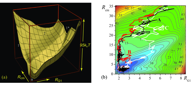
Figure 2: (a) Free energy surface for polymer collapse from state 2. Two clearly visible trenches belong to two distinct pathways connecting states 2 and 0. (b) Contour plot of the same free energy surface together with three typical collapse trajectories from state 2. $R_{\rm cm}$ and $R_{\rm G1}$ are introduced in the main text and shown in the units of $\sigma$.

To address this issue, we have completed a new analysis of free energies with two reaction coordinates that distinguish between states 1 and $1^{*}$. A choice of reaction coordinates which resolves all on-path and off-path metastable states consists of the radius of gyration $R_{\rm G1}$ of the subchain of monomers 1–36 and the distance $R_{\rm cm}$ between the centers of mass of subchains 55–100 and 1–12. To systematically investigate the conformational space associated with states 0, 1, $1^{*}$ and 2, we have performed numerous simulations in which $R_{\rm cm}$ and $R_{\rm G1}$ are bound to various centers $R_{\rm cm}^{0}$ and $R_{\rm G1}^{0}$ by harmonic potentials $u_{\rm h1}(R_{\rm cm})=0.5k_{1}(R_{\rm cm}-R_{\rm cm}^{0})^{2}$ and $u_{\rm h2}(R_{\rm G1})=0.5k_{2}(R_{\rm G1}-R_{\rm G1}^{0})^{2}$, where $k_{1}=k_{2}=0.5\varepsilon/\sigma^{2}$. In contrast to the constant force bias employed in Eq. (1), these harmonic potentials are sufficiently stiff to stabilize polymer trajectories on the steep slopes leading down to a deep free energy minimum, which allows an accurate measurement of the depth of this minimum and of the transition area. The $R_{\rm cm}$ and $R_{\rm G1}$ derivatives of the unbiased free energy $F(R_{\rm cm},R_{\rm G1})$ in the vicinity of each center $(R_{\rm cm}^{0},R_{\rm G1}^{0})$ are readily calculated from similar derivatives of the biased free energy $F^{*}(R_{\rm cm},R_{\rm G1},k_{1},R_{\rm cm}^{0},k_{2},R_{\rm G1}^{0})$ by subtracting from the latter $k_{1}(R_{\rm cm}-R_{\rm cm}^{0})$ and $k_{2}(R_{\rm G1}-R_{\rm G1}^{0})$, respectively. To establish the partial derivatives over the entire phase space we follow the scheme outlined for the 1D case and perform a linear weighted average of all available statistics from simulations with different $R_{\rm cm}^{0}$ and $R_{\rm G1}^{0}$. A free energy surface is computed numerically on a grid by minimizing the sum of squared deviations between its partial derivatives, represented by finite differences, and their numerical values obtained from simulations.

The result of this computation for $F(R_{\rm cm},R_{\rm G1})$ is shown in Fig. 2(a). The narrow trench that runs along the $R_{\rm cm}$ axis indicates the collapse transition from state 1 to 0, whereas the wide diagonal trench corresponds to the “unfolding” transition from state 0 to $1^{*}$. The accuracy of $F(R_{\rm cm},R_{\rm G1})$ is addressed in auxiliary material EPA where we examine the conformational transition between states 1 and $1^{*}$. Figure 2(b) shows the contour plot of $F(R_{\rm cm},R_{\rm G1})$ together with three representative trajectories for unconstrained ($k_{1}=k_{2}=0$) polymer collapse from state 2. Trajectory A in Fig. 2(b) follows the typical collapse pathway $2\to 1\to 0$. However, 683 out of the total of 10000 simulated collapse trajectories never enter the $1\to 0$ trench but instead reverse the “unfolding” pathway, similarly to trajectory C in Fig. 2(b).

When collapse proceeds along its typical path, a nonequilibrium effect is occasionally observed at the point when blobs 1–36 and 55–100 come into contact. As a result of vigorous mixing caused by the collision of the two blobs, monomers 27–36 may break from blob 1–36 and, subsequently, may either return to the same blob, as shown by trajectory B in Fig. 2(b), or join with blob 55–100, which appears as a sudden transition from state 1 to $1^{*}$ (not shown). Aside from this local nonequilibrium effect, we ask if the polymer is generally in quasi-equilibrium during its collapse, as assumed in diffusive model. To address this issue, in Fig. 3(a) we compare mean “equilibrium” and “nonequilibrium” times $t_{\rm eq}$ and $t_{\rm neq}$ of unimpeded polymer collapse from different initial positions in the $1\to 0$ trench. To compute $t_{\rm eq}$, we have run extensive simulations of the polymer bound to various positions in the trench by harmonic constraints $u_{\rm h1}$, $u_{\rm h2}$, that are lifted at regular times to initiate the total of 180000 independent collapse trajectories. $t_{\rm neq}$ are derived from other 10000 trajectories which originate in state 2 and traverse the $1\to 0$ trench in passing. The ratio $t_{\rm neq}/t_{\rm eq}$ in Fig. 3(a) shows a pronounced peak in the transition region between states 1 and 0, indicating delay in collapse caused by the local nonequilibrium effect described above. Furthermore, $t_{\rm neq}/t_{\rm eq}$ increases monotonically as $R_{\rm cm}\to 2.5\sigma$, which suggests that the freely collapsing polymer fails to achieve local equilibrium as it traverses steep portions of the reaction pathway.

We also find evidence that different portions of the free energy surface manifest different effective diffusion constants. Equilibrium times $t_{\rm eq}$ can be fitted to the 2D diffusive model with the diffusion coefficients $D_{1}=6.4\times 10^{-5}k_{\rm B}T\gamma^{-1}$ for $R_{\rm G1}$ and the position-dependent $D_{2}$ for $R_{\rm cm}$, shown in Fig. 3(b) EPA . Note that $D_{2}$ decreases by an order of magnitude when the polymer enters the free energy basin of its collapsed state, in agreement with the previous work on two-state protein folding where a similar slowdown in diffusion is attributed to the increasing polymer compactness Chahine et al. (2007). In experiments Waldauer et al. (2008) on the folding kinetics of protein L, a ten-fold slowdown in diffusion is observed after the initial hydrophobic collapse and attributed to the ruggedness of the energy landscape in the compact unfolded state. In the absence of a folding barrier, slow diffusion in the compact unfolded state may contribute significantly to the overall folding time, so that details of the energy landscape in this state may become very important. In the present case, a planar cut of the free energy surface in Fig. 3(b) indicates that the depth of the ground state basin is $\sim 20k_{\rm B}T$, too large to be computed from irreversible collapse trajectories. Estimating the drag coefficient $\gamma$ from Stokes’ formula, we find the mean diffusion coefficient $\overline{D_{2}}$ to be in good agreement with the value obtained from experiments on hydrophobic collapse of proteins Sadqi et al. (2003). This is not surprising since hydrophobic collapse of many heteropolymers involves diffusion and mutual aggregation of locally collapsed structures Lee and Thirumalai (2000), the same elementary processes that take part in the $1\to 0$ transition described by $D_{2}$.

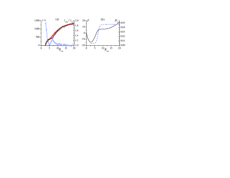
Figure 3: (a) Collapse times $t_{\rm eq}$ (squares) and $t_{\rm neq}$ (circles) from different initial positions in the $1\to 0$ trench. The solid curve is the fit of $t_{\rm eq}$ with $D_{1}=6.4\times 10^{-5}$, describing lateral vibrations of collapse trajectories in the trench, and $D_{2}$, shown as dash curve in (b). Triangles (right axis) are $t_{\rm neq}/t_{\rm eq}$. In (b), the solid curve is the planar cut $R_{\rm G1}=2\sigma$ of the 2D free energy surface. The units are $k_{\rm B}T$ for $F$, $\sigma$ for $R_{\rm cm}$ and $k_{\rm B}T\gamma^{-1}$ for $D_{1}$, $D_{2}$.

In closing, we can draw some general conclusions from the behavior of this relatively simple HP model. Most applications of the diffusive model to protein folding rely on the assumptions that i) the protein is in local equilibrium during its folding, ii) the energy landscape can be projected onto a single reaction coordinate, and iii) the effective diffusion coefficient is constant, with noted exceptions Chahine et al. (2007); Best and Hummer (2006). We have presented an efficient method for the calculation of multi-dimensional free energy surfaces that has allowed us to determine the validity of these assumptions when applied to hydrophobic collapse as a basic model for downhill protein folding. We find that polymer collapse generally adheres to the equilibrium energy landscape, although one cannot neglect nonequilibrium effects which, in the present case, noticeably delay collapse or cause it to take an altered pathway. Nonequilibrium features are not captured in equilibrium free energy calculations and can only be revealed by additional analysis of collapse trajectories. At the same time, nonequilibrium effects bias the free energy estimates that are obtained from collapse/folding trajectories. Irreversible conformational changes, associated with folding, also interfere with accurate determination of free energies from folding trajectories. Furthermore we find, in agreement with previous work Chahine et al. (2007); Waldauer et al. (2008), that diffusion slows down by an order of magnitude in the collapsed state, resulting from the increasing polymer compactness. In the case of downhill protein folding, this slow diffusion in the collapsed state may contribute significantly to the overall folding time. Finally, as illustrated by trajectory A in Fig. 2(b), fluctuations in the final state are not necessarily described by the same reaction coordinate as collapse to this state, so that projecting trajectories onto a single reaction coordinate may turn out to be inaccurate even in the case of a single apparent pathway. In the present study two reaction coordinates have proved sufficient to build a thermodynamically and kinetically consistent diffusive model with two distinct, physically meaningful diffusion coefficients.

This work was supported by NSF through Grant No. CHE-0517818 and through TeraGrid Grant No. TG-CHE070075N.

References

- Kramers (1940) H. A. Kramers, Physica 7, 284 (1940).
- (2) P. G. Wolynes, J. N. Onuchic, and D. Thirumalai, Science 267, 1619 (1995); J. N. Onuchic, Z. Luthey-Schulten, and P. G. Wolynes, Annu. Rev. Phys. Chem, 48, 545 (1997).
- (3) H. S. Chan and K. A. Dill, Proteins: Struct. Funct. Genet. 30, 2 (1998); K. A. Dill, Protein Sci. 8, 1166 (1999).
- (4) D. Thirumalai and S. A. Woodson, Acc. Chem. Res. 29, 433 (1996).
- (5) M. S. Z. Kellermayer, S. B. Smith, H. L. Granzier, and C. Bustamante, Science 276, 1112 (1997); J. M. Fernandez and H. Li, ibid. 303, 1674 (2004); M. T. Woodside, P. C. Anthony, W. M. Behnke-Parks, K. Larizadeh, D. Herschlag, and S. M. Block, ibid. 314, 1001 (2006).
- Chahine et al. (2007) J. Chahine, R. J. Oliveira, V. B. P. Leite, and J. Wang, Proc. Nat. Acad. Sci. USA 104, 14646 (2007).
- Best and Hummer (2006) R. B. Best and G. Hummer, Phys. Rev. Lett. 96, 228104 (2006).
- End (a) The average content of hydrophilic aminoacids in globular proteins is 43.6%, see T. E. Creighton, PROTEINS: Structures and Molecular Properties (W. H. Freeman and Company, New York, 1993), 2nd ed.
- End (b) Similar collapse scenarios were observed for 5 out of 6 generated sequences, which contained H stretches long enough to act as nucleation centers during collapse.
- Grest and Kremer (1986) G. S. Grest and K. Kremer, Phys. Rev. A 33, 3628 (1986).
- End (c) Differentiating with respect to eliminates additive constants in these functions that are customarily determined by solving a system of nonlinear equations, as in the Weighted Histogram Analysis method [A. M. Ferrenberg and R. H. Swendsen, Phys. Rev. Lett. 63, 1195 (1989)].
- (12) See EPAPS Document No. [] for additional discussion of the transition and for details of the fit of in Fig. 3(a). For more information on EPAPS, see http://www.aip.org/pubservs/epaps.html.
- Waldauer et al. (2008) S. A. Waldauer et al., HFSP J. 2, 388 (2008).
- Sadqi et al. (2003) M. Sadqi, L. J. Lapidus, and V. Muñoz, Proc. Nat. Acad. Sci. USA 100, 12117 (2003).
- Lee and Thirumalai (2000) N. Lee and D. Thirumalai, J. Chem. Phys. 113, 5126 (2000).