Four-dimensional variational assimilation in the unstable subspace (4DVar-AUS) and the optimal subspace dimension

Abstract

A key a priori information used in 4DVar is the knowledge of the system’s evolution equations. In this paper we propose a method for taking full advantage of the knowledge of the system’s dynamical instabilities in order to improve the quality of the analysis. We present an algorithm, four-dimensional variational assimilation in the unstable subspace (4DVar-AUS), that consists in confining in this subspace the increment of the control variable. The existence of an optimal subspace dimension for this confinement is hypothesized. Theoretical arguments in favor of the present approach are supported by numerical experiments in a simple perfect non-linear model scenario. It is found that the RMS analysis error is a function of the dimension $N$ of the subspace where the analysis is confined and is minimum for $N$ approximately equal to the dimension of the unstable and neutral manifold. For all assimilation windows, from 1 to 5 days, 4DVar-AUS performs better than standard 4DVar. In the presence of observational noise, the 4DVar solution, while being closer to the observations, if farther away from the truth. The implementation of 4DVar-AUS does not require the adjoint integration.

1 Introduction

Accuracy in the definition of the initial condition is an important factor for the performance of numerical weather and ocean prediction. The classical problem of estimating the state of a dynamical system from noisy and incomplete observations is known in meteorology and oceanography as data assimilation (Daley,, 1991; Kalnay,, 2003). The goal of data assimilation in the initialization process is to provide the best possible estimate of the present state of the system using the available, partial and noisy, observations and the approximate equations governing the system’s evolution. The estimate, referred to as the analysis, is obtained by optimally combining the information coming from a model forecast (background) and the observations (Talagrand,, 1997).

The non-linear stability properties of the system do not only determine the predictability horizon of the initial value problem but also profoundly influence the assimilation process, affecting directly its quality and that of the subsequent forecast (see e.g. Carrassi et al., 2008a, , and references therein). All assimilation methods, more or less implicitly, exert some control on the flow-dependent instabilities by means of the observational information. The Assimilation in the Unstable Subspace (AUS, Trevisan and Uboldi,, 2004) explicitly estimates the flow-dependent instabilities and makes use of the unstable subspace as additional dynamical information. The 4-dimensional extension of AUS is the main scope of the present paper. In Trevisan and Uboldi, (2004) and in other applications of the AUS assimilation, only a few unstable directions were tracked, whereas in the present study we make use of the entire unstable and neutral subspace, the subspace spanned by the Lyapunov vectors with positive and null exponents.

Assimilation methods can be classified in two categories: sequential and variational, the most notable in the two classes being Kalman Filters and 4DVar respectively (Ghil and Malanotte Rizzoli,, 1991; Kalnay,, 2003, and references therein). The Kalman Filter was originally developed for linear systems but a straightforward way of extending the linear results to the nonlinear case is given by the Extended Kalman Filter (EKF) (Jazwinski,, 1970; Miller et al.,, 1994).

Efficient minimization algorithms associated with adjoint techniques (Talagrand and Courtier,, 1987) facilitate the implementation of 4DVar, an established and powerful assimilation method for meteorology and oceanography. In many realistic circumstances, reduced-rank approximations or a Monte Carlo approach, the latter referred to as Ensemble Kalman Filter (EnKF) (Evensen,, 1994), have been adopted to circumvent the prohibitive cost of the full Extended Kalman Filter. The reader is referred to Kalnay, (2003) and Tsuyuki and Miyoshi, (2007) for a review on the state of the art of data assimilation in meteorology; see also Lorenc, (2003), Kalnay et al., (2007) and Gustafsson, (2007) for a discussion on the relative merits of 4DVar and EnKF.

The system’s unstable subspace and its role in the assimilation process are central to our discussion. Hence, we briefly comment on how the flow dependent instabilities are dealt with by Kalman type filters and 4DVar. In the Kalman filter, the propagation of the flow dependent instabilities is obtained by explicitly evolving the analysis error covariance from the previous analysis step. In Ensemble Kalman filters the subspace dimension of forecast error is at most equal to N-1, if N is the number of ensemble members: the rank deficiency of the background error information is partly alleviated by covariance localization if N is too small (Hamill et al.,, 2001). A related aspect is the filter divergence that appears particularly critical in relation to sampling error (Whitaker and Hamill,, 2002).

4DVar generates a model trajectory that best fits the observations available within a given assimilation window. Within the assimilation window, the flow dependent instabilities are naturally described by the forward integration of the model and backward integration of the adjoint that model the error evolution. In addition, at the start of each assimilation window, an a priori estimate of the background error covariance is needed (Bannister,, 2008).

For long assimilation windows, 4DVar analysis errors are known to project on the unstable subspace of the system (Pires et al.,, 1996). Errors in the stable directions that would be damped in the long range, for short assimilation windows are non-negligible in the analysis and affect the next assimilation cycle, causing short term enhanced error growth (Swanson et al.,, 2000). It therefore seems appropriate to avoid introducing such type of error: this can be achieved by confining the increment of the 4DVar control variable in the unstable and neutral subspace of the system. In this way we avoid reintroducing observational error in the stable directions at each assimilation step: we anticipate that this is beneficial only if observations are not perfect. In this paper we present an algorithm (4DVar-AUS) that minimizes the 4DVar cost function under the above constraint. The dynamical information on the growth of errors in the unstable and neutral directions, the Lyapunov vectors with positive and null exponents, is explicitly estimated and, as explained in Section 2.2.2, the adjoint integration is not needed.

The idea of confining the analysis increment in the unstable subspace is not new. The sequential algorithm, referred to as AUS, has been introduced by Trevisan and Uboldi, (2004). Its application to different models and observation configurations has shown that, even in the context of high-dimensional systems, an efficient error control and accurate state estimate can be obtained even by monitoring only a reduced number of unstable directions (Uboldi and Trevisan,, 2006; Carrassi et al.,, 2007; Carrassi et al., 2008b, ). The basic elements of the AUS scheme that differentiate it from other ensemble type Kalman filters are the explicit monitoring of the unstable directions of the system and the confinement of the analysis increment in the subspace that they span. A localization of the unstable structures, and consequently a localization of the error covariances (a feature common to other EnKF type methods) is necessary if the dimension of the subspace for the AUS assimilation is too small to describe the background error. The present extension of AUS to the four-dimensional case has the advantage of using the time distributed observations to track the instabilities that develop along the flow.

One of the main goals of the present study is to address the following question: is there an optimal subspace dimension for the assimilation and is this related to the dimension of the unstable subspace of the system? In order to address this question, 4DVar-AUS is formulated in a perfect model setting and using a subspace of variable dimension.

Theoretical arguments will be presented to indicate that the subspace dimension should at least be equal to the unstable manifold dimension.

Results of the application of 4DVar-AUS to simple perfect non-linear systems obtained by varying the number of degrees of freedom in the Lorenz $40$-variable model (Lorenz,, 1996) will be presented. The relation between the optimal subspace dimension and the number of positive exponents will be numerically investigated and it will be shown that the results confirm the theoretical arguments.

The paper is organized as follows: the formulation of 4DVar-AUS and theoretical arguments on the subspace optimization are introduced in Section 2; results of the application to the Lorenz, (1996) model are presented in Section 3, while conclusions are drawn in Section 4.

2 Formulation of 4DVar in the unstable subspace

2.1 4DVar

Strong constraint 4DVar seeks the (nonlinear) best estimate of the initial state ${\bf x}_{0}$ that minimizes the misfit with observations in a given time interval (window) and possibly with a background state ${\bf x}_{0}^{b}$. The standard cost function for strong constraint 4DVar, in discrete form, can be written as:

$$\begin{split}J({\bf x}_{0})&=({\bf x}_{0}-{\bf x}^{b}_{0})^{T}{\bf B}^{-1}({\bf x}_{0}-{\bf x}^{b}_{0})+\\ &+\sum_{i=0}^{n}({\cal H}_{i}{\bf x}_{i}-{\bf y}_{i}^{o})^{T}{\bf R}^{-1}({\cal H}_{i}{\bf x}_{i}-{\bf y}_{i}^{o})\end{split}$$ (1)

where ${\bf y}^{o}_{i}$ are the observations available at discrete times $t_{i}=i{\Delta t},i=0,...,n$ , within the assimilation window of length $\tau=t_{n}-t_{0}$; $\bf B$ and $\bf R$ represent the background and observation error covariance matrices, ${\cal H}$ the nonlinear observation operator, and the sequence of model states ${\bf x}_{i}$ is a solution of the nonlinear model equations:

$${\bf x}_{i}={\cal M}_{0\rightarrow i}({\bf x}_{0}),$$ (2)

The control variable for the minimization is the model state ${\bf x}_{0}$ at the beginning of the assimilation window.

Given the tangent linear equations describing the evolution of infinitesimal perturbations $\delta{\bf x}_{i}$ relative to an orbit of Eq. (2):

$$\delta{\bf x}_{i}={\bf M}_{0\rightarrow i}\delta{\bf x}_{0},$$ (3)

the gradient of $J$ with respect to ${\bf x}_{0}$ can be written as:

$$\begin{split}\frac{1}{2}\nabla_{{\bf x}_{0}}J&={\bf B}^{-1}({\bf x}_{0}-{\bf x}^{b}_{0})+\\ &+\sum_{i=0}^{n}{\bf M}_{0\rightarrow i}^{T}{\bf H}_{i}^{T}{\bf R}^{-1}({\cal H}_{i}{\bf x}_{i}-{\bf y}_{i})\end{split}$$ (4)

where ${\bf H}_{i}$ represents the linearized observation operator, and the superscript $T$ stands for transpose.

For a given nonlinear trajectory, the gradient can be estimated by use of the adjoint method (Le Dimet and Talagrand,, 1986).

The solution of the minimization problem is obtained by forward integration of the model and backward integration of the adjoint, with an iterative descent algorithm.

2.2 4DVar-AUS

2.2.1 Unstable subspace and computation of Lyapunov vectors

Lyapunov vectors, defined for nonlinear systems, are the time dependent physical structures associated with the Lyapunov exponents. There are basically two definitions of Lyapunov vectors that span the same invariant Oseledec subspaces. The first is that of an orthonormal set of vectors, the eigenvectors of the limit operator (Oseledec,, 1968):

$${\bf\Phi}_{\infty}(t)=\lim_{t_{0}\rightarrow-\infty}[{\bf M}_{t_{0}\rightarrow t}{\bf M}_{t_{0}\rightarrow t}^{*}]^{\frac{1}{2(t-t_{0})}}$$ (5)

where ${\bf M}^{*}$ is the adjoint operator and the initial state, ${\bf x}_{0}$ of the nonlinear trajectory is on the attractor (for further reference in the meteorological literature see Lorenz, (1984) and Legras and Vautard, (1996)).

The second is a set of non-orthogonal Lyapunov vectors, that are independent of the norm and map into themselves with the tangent linear propagator (Eckmann and Ruelle,, 1985; Brown et al.,, 1991). These vectors have been shown to be the natural generalization of eigenvectors and Floquet vectors to aperiodic flow (Trevisan and Pancotti,, 1998).

The following standard technique is commonly used for calculating the orthonormal set of Lyapunov vectors (Benettin et al.,, 1980): a set of $N$ initially random tangent vectors are linearly evolved and orthonormalized every $\tau$ time units. After a spin-up time these vectors span the $N$-dimensional most unstable subspace of the system.

An efficient method for recovering norm-independent non-orthogonal Lyapunov vectors is given by Wolfe and Samelson, (2007). Either one of the two above-mentioned methods can be used to identify the unstable, neutral, stable subspaces, the span of Lyapunov vectors with positive, null, negative exponents; the former, simpler technique will be adopted in the present application.

In weather prediction, bred vectors (Toth and Kalnay,, 1993, 1997) are usually computed instead of Lyapunov vectors. Bred vectors are the finite amplitude generalization of Lyapunov vectors and are computed as differences between twin nonlinear model integrations. The re-normalization amplitude and breeding time are the parameters being tuned to select the instability scale. With an infinitesimal re-normalization amplitude and periodic orthonormalization the bred vectors algorithm would produce the same results as the Lyapunov vectors algorithm of Benettin et al., (1980).

In previous applications of AUS (see e.g. Carrassi et al., 2008b, , and references therein) to more realistic atmospheric and oceanic models, the unstable vectors were computed with the breeding technique. In those works, only a small number of bred vectors was used at each assimilation time. Because of the low dimensionality of the subspace spanned by those bred vectors a space localization was needed; furthermore, the breeding method was applied to the assimilation system instead of the freely evolving system in order to select those instabilities that survived the previous assimilation.

In the present application we use the entire unstable and neutral subspace of the freely evolving system and we do not need any localization.

2.2.2 The 4DVar-AUS algorithm

The approach consists in determining the increment $\delta{\bf x}_{0}$ which minimizes the cost function in the reduced dimension subspace spanned by the $N$ most unstable directions of the system corresponding to the leading $N$ Lyapunov exponents.

After a transient time, the numerical technique described in Section 2.2.1 (Benettin et al.,, 1980) leads to the identification of an orthonormal set of vectors spanning the $N$-dimensional most unstable subspace. We apply this procedure to the solution of the assimilation cycle, starting initially with $N$ arbitrarily chosen tangent vectors. The Gram-Schmidt orthonormalization is applied at the end of each assimilation interval $\tau$.

Let ${\bf E}_{0}$ be the matrix whose columns are the orthonormal tangent vectors spanning the $N$-dimensional most unstable subspace of the system at $t_{0}$. The linear evolution within the assimilation window $[t_{0},\tau]$ is given by:

$${\bf M}_{0\rightarrow i}{\bf E}_{0}={\bf E}_{i}{\bf\Lambda}_{i},(i=0,...,n)$$ (6)

where

$$\begin{split}{\bf\Lambda}_{i}&=diag\biggl{[}exp\int_{t_{0}}^{t_{i}}\lambda^{(1)}(t)dt,exp\int_{t_{0}}^{t_{i}}\lambda^{(2)}(t)dt,...,\\ &,...,exp\int_{t_{0}}^{t_{i}}\lambda^{(N)}(t)dt\biggr{]}\end{split}$$ (7)

and $\lambda^{(j)}(t)$ is the $j^{th}$ local exponent.

Consider the projection of the increment $\delta{\bf x}_{0}$ in the subspace defined by ${\bf E}_{0}$. In general, given a norm defined by the symmetric positive definite matrix ${\bf Q}$, the projection can be written as ${\bf E}_{0}({\bf E}^{T}_{0}{\bf Q}{\bf E}_{0})^{-1}{\bf E}_{0}^{T}{\bf Q}\delta{\bf x}_{0}$. For simplicity, in the following we adopt the Euclidean norm and we recall that the columns of ${\bf E}_{0}$ are orthonormal vectors.

Thus, let the increment $\delta{\bf x}_{0}$ be confined in the subspace ${\bf E}_{0}$ and its projection $\widetilde{\delta{\bf x}}_{0}$ be given by:

$$\widetilde{\delta{\bf x}}_{0}={\bf E}_{0}{\bf E}_{0}^{T}\delta{\bf x}_{0}$$ (8)

The evolution of the projected increment is governed by:

$$\widetilde{\delta{\bf x}}_{i}={\bf M}_{0\rightarrow i}{\bf E}_{0}{\bf E}_{0}^{T}\delta{\bf x}_{0}={\bf E}_{i}{\bf\Lambda}_{i}{\bf E}_{0}^{T}\delta{\bf x}_{0},(i=0,...,n)$$ (9)

Variations of the cost function (1) due to variations of the control variable $\widetilde{\delta{\bf x}}_{0}$ can be written as:

$$\begin{split}\widetilde{\delta{\bf J}}&=(\nabla_{x_{0}}J)^{T}\widetilde{\delta{\bf x}}_{0}\\ &=(\widetilde{\nabla_{x_{0}}J})^{T}{\bf\delta x}_{0}\end{split}$$ (10)

where the tilde represents the projection into the subspace ${\bf E}_{0}$, i.e. $\widetilde{\nabla_{x_{0}}J}={\bf E}_{0}{\bf E}_{0}^{T}\nabla_{x_{0}}J$.

Using (4) and (6), the cost function gradient in the reduced subspace becomes:

$$\begin{split}\frac{1}{2}\widetilde{\nabla_{{\bf x}_{0}}J}&={\bf E}_{0}\biggl{[}{\bf E}_{0}^{T}{\bf B}^{-1}({\bf x}_{0}-{\bf x}^{b}_{0})+\\ &+\sum_{i=0}^{n}{\bf\Lambda}_{i}{\bf E}_{i}^{T}{\bf H}_{i}^{T}{\bf R}^{-1}(\mathcal{H}_{i}{\bf x}_{i}-{\bf y}_{i})\biggr{]}\end{split}$$ (11)

An assimilation cycle is constructed by initializing the next assimilation window with the state and its associated unstable subspace estimates at the end of the previous window.

If $k$ indicates the index of the assimilation cycle and recalling that $\tau=t_{n}-t_{0}$:

${{\bf x}^{b}_{0}}(k+1)={\bf x}_{\tau}(k)$, where

$${\bf x}_{\tau}(k)={\cal M}_{0\rightarrow n}(k)({\bf x}_{0}(k))$$ (12)

and ${\bf E}_{\tau}(k)={\bf E}_{0}(k+1){\bf T}$, where

$${\bf M}_{0\rightarrow n}(k){\bf E}_{0}(k)={\bf E}_{\tau}(k){\bf\Lambda}_{\tau}(k)$$ (13)

and ${\bf T}$ is the upper triangular orthonormalization matrix.

In summary, the assimilation cycle is performed through the following steps:

1. A descent algorithm is used to find the cost function minimum by:

   1. forward integration of the nonlinear model using (2) to compute ${\bf x}_{i}$, starting from ${\bf x}_{0}^{b}$ at first iteration step;

   2. forward integration of the perturbations ${\bf E}_{0}$ using (6) to compute ${\bf E}_{i}$ and ${\bf\Lambda}_{i}$;

   3. estimate of $\widetilde{\nabla_{{\bf x}_{0}}J}$ from (11) and of $J$ from (1);

2. The nonlinear model is integrated starting from the minimizing solution ${\bf x}_{0}(k)$ to produce the analysis, ${\bf x}_{\tau}(k)$ (12).

3. The perturbations ${\bf E}_{0}(k)$ are evolved along the minimizing trajectory to produce ${\bf E}_{\tau}(k)$ (13);

4. The columns of ${\bf E}_{\tau}(k)$ are orthonormalized and stored in ${\bf E}_{0}(k+1)$ to be used in the next assimilation cycle;

5. ${\bf x}_{0}^{b}(k+1)$ is set equal to ${\bf x_{\tau}}(k)$.

Notice that no use of the adjoint integration is made.

In the 4DVar-AUS assimilation, the analysis increment is confined in the $N$-dimensional most unstable subspace of the previous analysis solution, with $N$ approximately equal to the number of positive and null Lyapunov exponents.

Theoretical arguments given in Section 2.3, confirmed by numerical results presented in Section 3, will show that during a 4DVar-AUS assimilation cycle, errors in the stable directions are damped and errors in the analysis solution are confined within the unstable and neutral manifold of the system. This subspace is locally parallel to the attractor (Eckmann and Ruelle,, 1985), so that one can find a state belonging to a nearby trajectory by moving along the tangent unstable directions.

2.3 Full space and reduced order covariance matrix of the assimilation error

The effect of the confinement on the expected assimilation error covariance is now examined.

Pires et al., (1996) investigated the behavior of the observational term of the cost function in chaotic systems, making the tangent linear hypothesis and observing the whole state. They showed that, using the assumption that the observation error is uncorrelated in time and isotropic, with variance $\sigma_{o}^{2}$, the covariance matrix ${\bf C}_{0}=<{\bf\eta}^{a}_{0}{\bf\eta}^{aT}_{0}>$ of the assimilation error ${\bf\eta}^{a}_{0}$ at $t=t_{0}$, $<>$ being the expectation operator, can be written as:

$${\bf C}_{0}=\sigma_{o}^{2}\left(\sum_{i=0}^{n}{\bf M}_{0\rightarrow i}^{T}{\bf M}_{0\rightarrow i}\right)^{-1}$$ (14)

By confinement in the subspace defined by the $N$ column vectors in ${\bf E}_{0}$ and using (6) one easily obtains the following expression for the covariance of the assimilation error:

$${\bf C}_{0}=\sigma_{o}^{2}{\bf E}_{0}(\sum_{i=0}^{n}{\bf\Lambda}_{i}{\bf E}_{i}^{T}{\bf E}_{i}{\bf\Lambda}_{i})^{-1}{\bf E}_{0}^{T}$$ (15)

To this point, no hypothesis has been made on the choice of ${\bf E}_{0}$ in (15). If the number $N$ of vectors of ${\bf E}_{0}$ is equal to the total number, $I$, of degrees of freedom of the system, (15) represents the covariance matrix in the full space.

Now let the $N$ column vectors of ${\bf E}_{0}$ be the Lyapunov vectors corresponding to the $N$ largest Lyapunov exponents. Assume that the Lyapunov vectors are orthogonal at $t_{0}$ (or have been orthonormalized) and assume, for the sake of simplicity, that they remain orthogonal within the time window, then:

$$\begin{split}&{\bf C}_{0}=\sigma_{o}^{2}{\bf E}_{0}{\bf D}_{0}{\bf E}_{0}^{T}\\ &=\sigma_{o}^{2}{\bf E}_{0}diag\biggl{\{}\bigl{[}\sum_{i=0}^{n}({\bf\Lambda}_{i}^{(1)})^{2}\bigr{]}^{-1},\bigl{[}\sum_{i=0}^{n}({\bf\Lambda}_{i}^{(2)})^{2}\bigr{]}^{-1},...,\\ &,...,\bigl{[}\sum_{i=0}^{n}({\bf\Lambda}_{i}^{(N)})^{2}\bigr{]}^{-1}\biggr{\}}{\bf E}_{0}^{T}\end{split}$$ (16)

where ${\Lambda}_{i}^{(j)}=exp\int_{t_{0}}^{t_{i}}\lambda^{(j)}(t)dt$.

At time $\tau=t_{n}$, the analysis error covariance $C_{\tau}=<{\bf\eta}^{a}_{\tau}{\bf\eta}^{aT}_{\tau}>$ under the tangent linear assumption, is:

$$\begin{split}&{\bf C}_{\tau}=\sigma_{o}^{2}{\bf E}_{\tau}{\bf D}_{\tau}{\bf E}_{\tau}^{T}\\ &=\sigma_{o}^{2}{\bf E}_{\tau}diag\biggl{\{}\bigl{[}\sum_{i=0}^{n}({\bf\Lambda}_{i}^{(1)})^{-2}\bigr{]}^{-1},\bigl{[}\sum_{i=0}^{n}({\bf\Lambda}_{i}^{(2)})^{-2}\bigr{]}^{-1},...,\\ &,...,\bigl{[}\sum_{i=0}^{n}({\bf\Lambda}_{i}^{(N)})^{-2}\bigr{]}^{-1}\bigg{\}}{\bf E}_{\tau}^{T}\end{split}$$ (17)

where ${\bf E}_{\tau}={\bf E}(t_{n})$.

In the expressions for ${\bf C}_{0}$ and ${\bf C}_{\tau}$, the role of the amplifying and decaying modes is interchanged. The generic term $(D_{0})_{j,j}$ of the diagonal matrix ${\bf D}_{0}$, representing the analysis error covariance associated with the $j^{th}$ Lyapunov direction (the $j^{th}$ column of ${\bf E}(t_{0})$, ${\bf e}_{j}(t_{0})$) at the beginning of the assimilation window, $t=t_{0}$ is:

$$\begin{split}(D_{0})_{j,j}=\sigma_{o}^{2}\bigl{\{}1+[exp(\lambda^{(j)}\Delta t)]^{2}&+[exp(\lambda^{(j)}2\Delta t)]^{2}+\\ &+...+[exp(\lambda^{(j)}n\Delta t)]^{2}\bigr{\}}^{-1}\\ &=\sigma_{o}^{2}\frac{1-e^{2\lambda^{(j)}\Delta t}}{1-e^{2(n+1)\lambda^{(j)}\Delta t}}\end{split}$$ (18)

where $\lambda^{(j)}$ is the $j^{th}$ local Lyapunov exponent assumed, to simplify notation, to be constant within the assimilation window and $\Delta t$ is the time interval between observations. A similar expression holds at the end of the assimilation window, $t=\tau$:

$$\begin{split}(D_{\tau})_{j,j}=\sigma_{o}^{2}\bigl{\{}1+[exp(-\lambda^{(j)}\Delta t)]^{2}&+[exp(-\lambda^{(j)}2\Delta t)]^{2}+\\ &+...+[exp(-\lambda^{(j)}n\Delta t)]^{2}\bigr{\}}^{-1}\\ &=\sigma_{o}^{2}\frac{1-e^{-2\lambda^{(j)}\Delta t}}{1-e^{-2(n+1)\lambda^{(j)}\Delta t}}\end{split}$$ (19)

where, now, large $n$ refers to earlier times.

In agreement with Pires et al., (1996), the influence of observational error on the stable (unstable) directions is damped as time increases (decreases) within the assimilation interval. At $t=\tau$ ($t=t_{0}$), the largest error is along the most unstable (stable) directions; the older (more recent) observations, corresponding to increasing $n$, give smaller and smaller contributions. For sufficiently long assimilation windows the error along the stable (unstable) directions is damped.

2.4 On the optimal subspace dimension

Now, we focus on the effect on the analysis error covariance of the assimilation in the reduced, unstable and neutral subspace. In 4DVar-AUS, the analysis increment is confined in the subspace of the $N$ most unstable directions: let $N$ be equal to $N^{+}+N^{0}$, where $N^{+}$ and $N^{0}$ are the number of positive and null Lyapunov exponents. The influence of errors in stable directions, ${\bf e}_{N^{+}+N^{0}+1},{\bf e}_{N^{+}+N^{0}+2},..{\bf e}_{I}$ on the analysis error is eliminated by the confinement. Because we do not make corrections in the stable directions we avoid introducing, at every assimilation step, errors in the assimilation solution that project on the stable subspace. In this way, errors in the stable directions can naturally decay along the cycle. In standard 4DVar, instead, errors in the observations produce errors in the assimilation solution that project on the stable directions at each assimilation step.

Results presented in the next section confirm these arguments, showing that the confinement in the unstable subspace is indeed beneficial to the performance of the assimilation. At final time of sufficiently long assimilation windows analysis errors in the stable directions would be damped also in standard 4DVar; however, this cannot be achieved in practice because nonlinearities set a limit to the window extension that can be used.

Swanson et al., (2000) investigated the effect of various observational errors on the 4DVar analysis and pointed out that errors in the stable directions can cause short term enhanced growth with adverse effect on the forecast. Their results are in agreement with the present findings.

The effect of the confinement on the efficiency of the numerical algorithm is discussed in Appendix A.

3 Application to the Lorenz (1996) model

3.1 Model and experimental setting

The results presented in this section are based on the low-order chaotic model of Lorenz, (1996) and Lorenz and Emanuel, (1998). The model is a simple analogue of mid-latitude atmospheric dynamics and its variables represent the values of a meteorological quantity at $I$ equally spaced geographic sites on a periodic latitudinal domain.

The governing equations are:

$$\frac{d}{dt}x_{j}=(x_{j+1}-x_{j-2})x_{j-1}-x_{j}+F$$ (20)

with $j=1,...,I$.

Following Lorenz and Emanuel, (1998) we set the external forcing $F=8$, a value giving rise to chaotic behavior. In this paper we consider three model configurations with different numbers of degrees of freedom $I$. For $I=40,60,80$ the three systems have $13,19,26$ positive Lyapunov exponents, respectively. The doubling time associated to the leading Lyapunov exponent $\lambda^{(1)}$ is, in all three systems, approximately equal to $2$ days if the system time unit corresponds to $5$ days.

Figure 1: Time average RMS analysis error at $t=\tau$ as a function of the subspace dimension $N$ for three model configurations: $I$=$40$, $60$, $80$. Different curves in the same panel refer to different assimilation windows from 1 to 5 days. The observation error standard deviation is $\sigma_{o}=0.2$.

Observing system simulation experiments are performed in a perfect model environment: a trajectory on the attractor of the system is assumed to represent the truth. Observations are created by adding to the true state Gaussian distributed random errors with variance $\sigma_{o}^{2}$.

The observational network is the same as in Fertig et al., (2007). An observation is placed in one out of four grid points at each observation time. The frequency of observation is $1.5$ hours, and the observed grid points are rotated so that, in a six hours interval, all grid points are observed once.

An analysis cycle is set up with contiguous assimilation windows so that the initial time $t_{0}$ in one window corresponds to the last time $t_{n}=\tau$ of the previous one, as described in Section 2.2.2. Experiments are performed using assimilation windows $\tau=1,...,5$ corresponding to $1,...,5$ days. In each experiment the analysis cycle consists of $5000$ consecutive windows. A Conjugate Gradient algorithm (Press et al.,, 1992, Chap. 10) is used for the minimization of the cost function at each step of the algorithm of both 4DVar and 4DVar-AUS.

The time mean, over an assimilation cycle of $5000$ windows, of the RMS analysis error obtained with standard 4DVar is compared with that obtained by means of the 4DVar-AUS algorithm. The latter is applied using a variable number $N$ of directions in order to find the optimal subspace dimension for the confinement.

3.2 Results

Following the theoretical approach of Pires et al., (1996), a first set of experiments is performed without background term in the cost function. The 4DVar-AUS algorithm described in Section 2.2.2 requires the definition of the background (i. e. the estimate produced by the previous assimilation cycle) and of the subspace ${\bf E}_{0}$ representing instabilities at the end of the trajectory in the previous window. Therefore, even in the absence of an explicit background term in the cost function, the solution relative to one window is dependent on the solution of the previous one. For the first set of experiments an assimilation cycle is set up by successive minimizations of the observational part of the cost function only. We recall that the initial guess of the control variable at $t=t_{0}$ is equal to the analysis at $t=\tau$ of the previous assimilation and, in the 4DVar-AUS algorithm, the $N$ column vectors of ${\bf E}_{0}$ are obtained by orthonormalizing the vectors ${\bf E}_{\tau}$.

The results of 4DVar-AUS are compared with standard 4DVar. The RMS analysis error is computed at the end of each assimilation window and averaged over $5000$ successive assimilation windows. Experiments are performed with the three systems with $I=40,60$ and $80$ degrees of freedom; the number of null Lyapunov exponents of these systems is $N^{0}=1$ and the number of positive exponents is $N^{+}=13,19,26$, respectively.

Figure 2: Time average RMS analysis error at $t=\tau$ as a function of the length of the assimilation window for three model configurations: $I$=$40$, $60$, $80$. Different curves in the same panel refer to a different subspace dimension $N$ of 4DVar-AUS and to standard 4DVar. $\sigma_{o}=0.2$.

3.2.1 Error dependence on the subspace dimension

Figure 1 shows the mean RMS error as a function of the dimension $N$ of the subspace ${\bf E}_{0}$. Each panel refers to a different model configuration, $I=40,60,80$. When $N=I$ the error is that of standard 4DVar (one can either set $N=I$ in the 4DVar-AUS scheme or use the standard 4DVar algorithm: the results are the same within numerical accuracy). The value of $\sigma_{o}$ is set to $0.2$ (the ’climatological’ standard deviation for the system is about $5.1$).

When $N$ is smaller than the number of positive Lyapunov exponents, $N^{+}$, the 4DVar-AUS algorithm does not converge or gives very poor results. When $N$ is increased above this threshold, the error abruptly decreases and then gradually increases again up to the value obtained with standard 4DVar ($N=I$). Recalling that the number of positive global Lyapunov exponents for $I=40,60$ and $80$ is $13,19$ and $26$ respectively, the error minimum is obtained in all three model configurations for a value of $N$ approximately equal to $N^{+}+N^{0}$. Because the value of local Lyapunov exponents fluctuates around the respective global value, even moderately decaying directions can be locally expanding and a number $N$ a few units larger than $N^{+}+N^{0}$ is needed.

The most important result is that the minimum value of the error is obtained for an optimal subspace dimension which is very close to the number of positive and null Lyapunov exponents of the three ($40,60$ and $80$-variable) systems.

Notice the internal consistency of the results of Fig. 1: the value of the average RMS error is virtually the same in the three model configurations. In fact, dynamically, the three models are equivalent and have the same instabilities, but a different number $N^{+}$ of unstable directions are present in proportion to the extension of the spatial domain. Because the observational configuration is the same, with a number of observations proportional to the domain size, and using the value of $N$ appropriate for each system (given the respective value of $N^{+}$), we obtain the same accuracy of the analysis solution.

Figure 2 displays the experimental data as a function of $\tau$, to illustrate the improvement obtained with the 4DVar-AUS scheme for different assimilation windows. Because the stable directions have a negative impact on the quality of the assimilation, the error appears to decrease by successively discarding a larger number of (the most stable) directions. We argued that errors in the stable directions do not affect the analysis for long enough (relative to the decay rate) assimilation windows. In agreement with this conjecture, Fig. 2 shows that the improvement obtained by using the optimal value of $N$, and thus eliminating the stable components of the error, is largest for the shortest assimilation windows: the largest improvement, a $30\%$ reduction of the error with respect to classical 4DVar is obtained for the smallest $\tau$ corresponding to one day, while the improvement becomes less significant for larger $\tau$, and is about $20\%$ for the five days window.

The experiments were repeated using larger values of $\sigma_{o}=1$ and $\sqrt{2}$ and similar results were obtained (not shown) except that, as expected, the error scales with $\sigma_{o}$. It was not possible to complete all the experiments with a window of five days and the larger value of $\sigma_{o}$ because the algorithm failed due to increased nonlinearity; in addition, the error minimum is shifted to slightly larger values of $N$: these were, for instance equal to $17$, $25$ and $30$ for the $40$, $60$ and $80$-variable systems respectively when the largest observational error value ($\sigma_{o}=\sqrt{2}$) was used. This can be explained by noting that, when the error of the initial guess is larger, also the estimate of the unstable directions is less accurate at $t=t_{0}$; in such case a slightly larger subspace is needed.

3.2.2 Stable and unstable error components within the assimilation window

The time dependence of the error within the assimilation window, shown in Fig. 3 confirms the theoretical results of Section 2.3 and provides further insight on the reasons why 4DVar-AUS performs better than 4DVar. In the figure we show the 4DVar and 4DVar-AUS total error and the error projection on the stable directions ${\bf e}_{N^{+}+N^{0}+1},...,{\bf e}_{I}$, averaged over $5000$ consecutive assimilation windows. The results shown were obtained with two values of $\sigma_{o}=10^{-5}$ and $.2$, small enough that the analysis error scales with the observational error as predicted by the tangent linear theory of Section 2.3.

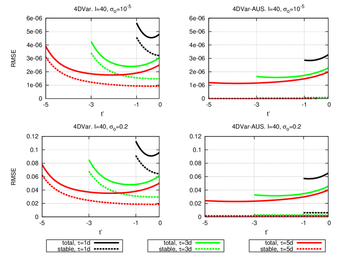
Figure 3: Time average RMS error within $1,3,5$ days assimilation windows as a function of $t^{\prime}=t-\tau$, with $\sigma_{o}=.2,10^{-5}$ for the model configuration $I=40$. Left panel: 4DVar. Right panel: 4DVar-AUS with $N=15$. Solid lines refer to total assimilation error, dashed lines refer to the error component in the stable subspace ${\bf e}_{16},...,{\bf e}_{40}$.

Figure 3 shows that, according to the theory, the 4DVar error is relatively larger in the stable subspace at initial time and in the unstable and neutral subspace at final time. Instead, in 4DVar-AUS errors are very small in the stable directions and project almost totally on the unstable and neutral subspace.

The 4DVar-AUS assimilation error is smaller than the 4DVar error particularly for short assimilation windows.

Because the search of the minimum of the 4DVar cost function is conducted in the entire phase space, its minimum cannot be larger than the minimum of the 4DVar-AUS cost function: this is confirmed by experimental evidence, the 4DVar cost function being typically a few percent smaller than the 4DVar-AUS cost function. We conclude that the 4DVar solution is closer to the observations but farther away from the real trajectory than the 4DVar-AUS solution. This is due to the fact that, in 4DVar, errors in the stable directions are “kept alive” by the observational error. In 4DVar-AUS, errors in the stable directions being never corrected, are naturally damped along the assimilation cycle: as a consequence, on average errors project only on the long term Lyapunov vectors contained in the matrix ${\bf E}_{0}$.

Results obtained by setting $\sigma_{o}=0$ show that the analysis error tends to zero in a time span that is shorter for standard 4DVar than for 4DVar-AUS; thus with perfect observations the full space 4DVar assimilation performs better, strengthening our conclusions. It is worth mentioning that the evolution of ${\bf E}_{0}$ is a key factor for the performance of the assimilation: in fact, experiments performed by using any number $N<I$ of random directions show that the error is always larger than the error of the full space 4DVar assimilation ($N=I$).

3.2.3 Inclusion of the background term

The 4DVar-AUS algorithm, in the absence of an explicit background term, amounts to assuming that the background error covariance matrix B is infinite in the unstable and neutral space, and $0$ in the stable subspace. The full 4DVar-AUS algorithm, still in the absence of an explicit background term, amounts to assuming that the matrix B is globally infinite. For completeness, a set of experiments was conducted with the inclusion of an explicit finite background term in the cost function. The static background error covariance matrix $\bf B$ was optimized for each assimilation window by the following iterative procedure. Starting from an initial guess, ${\bf B}$ is updated at each iteration step with the covariance of the difference between the forecast and true state, estimated from an assimilation cycle of 1000 consecutive windows. The process is repeated until convergence is obtained; in practice the iteration stops when the analysis error, averaged over the 1000 windows cycle, converges to an approximately constant value. To reduce the burden of computations $\bf B$ is optimized for each window only for standard 4DVar ($N=I$); the same matrix is used for the 4DVar-AUS experiments with the same window: in this way 4DVar-AUS is penalized, since its results could only improve if we used a matrix $\bf B$ specifically optimized for each given subspace dimension $N<I$.

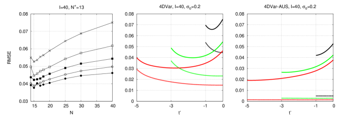
Figure 4: Left, middle and right panels same as: left panel of Fig. 1 and bottom left and right panels of Fig. 3 respectively, but for experiments with background term in the cost function. $\bf B$ was optimized as explained in the text.

Results are shown in Fig. 4, to be compared with Fig. 1 (for $I=40$) and with Fig. 3 (for $\sigma_{o}=0.2$). Everything else being equal, the introduction of the background term leads to an overall improvement of the performance in all experiments (compare the middle panel of Fig. 4 with the the lower left panel of Fig. 3 as concerns full 4DVar, and the right panel of Fig. 4 with the lower right panel of Fig. 3 as concerns 4DVar-AUS). This shows that useful information is contained in the matrix $\bf B$. The most accurate analysis is still obtained for a value of $N$ that is just above the number of positive and null Lyapunov exponents. It is seen that, in agreement with the theory, the largest improvements are obtained for shorter windows and for standard 4DVar. As expected, increasing the length of the time window decreases the influence of the background term. For 4DVar, the effect of the background term is particularly efficient in reducing the analysis error along the stable directions. Therefore a significant reduction of the error at the beginning of the time window is observed, but errors are nevertheless still present in the analysis in the stable directions. The conclusions to be drawn as to the matrix $\bf B$ as it has been defined here are first, as said, that it contains useful information in both the stable and unstable subspaces. Now, the error in the stable subspace is only partially decreased in the full 4DVar, while it is entirely eliminated in 4DVar-AUS. So, the description that the matrix $\bf B$ gives of the error in the stable subspace is more accurate than assuming that this error is infinite, but less accurate than assuming it is zero.

4 Conclusions

One of the main purposes of the present paper has been the development of four-dimensional variational assimilation in the unstable subspace. The results provide a proof-of-concept, at least in the case of the simple model used in this study, of the benefit in terms of assimilation performance of selecting the subspace where instabilities develop. The key result of this study is the existence of an optimal subspace dimension for the assimilation that is directly related to the unstable and neutral subspace dimension. The selected subspace - the leading Lyapunov vectors subspace - contains the most rapidly growing perturbations. In the presence of observational error, the optimal number of directions is approximately equal to $N^{+}+N^{0}$, where $N^{+}$ and $N^{0}$ are the number of positive and null Lyapunov exponents. The 4DVar solution ($N=I$), while being closer to the observations, is farther away from the truth. This result has been explained showing that, when we assimilate in the unstable and neutral subspace, errors in the stable directions are naturally damped. Because of observational error, assimilating in the whole space otherwise keeps the stable components of the error alive, deteriorating the overall assimilation performance. If the observational error is zero, the optimal dimension is the dimension $I$ of the whole space.

The present theoretical results can have implications for the application of advanced assimilation methods to high-dimensional models of the atmosphere and ocean. Here, we have shown that 4DVar could benefit from the dynamical information on the unstable directions - the “optimal” subspace where the analysis error is confined - propagated along the assimilation cycle. The possible application of the present findings to more realistic contexts is left for future investigations. Work is in progress to explore the existence of an optimal subspace dimension for EnKFs.

The results presented in this paper have been obtained with a simple and economical numerical model and, strictly speaking, do not prove anything as to what would be obtained with a more realistic model of the atmospheric flow. At the same time, the considerations which have led to the design of the experiments described in the paper, and which are confirmed by the results that have been obtained, are very general, and do not fundamentally require anything else than the existence of both stable and unstable modes in the system?? under consideration. One possible source of difficulties could be the unavoidable presence of errors in the assimilating model. The experiments described here have been performed under the hypothesis of a perfect model. In the more realistic situation of an imperfect model, the corresponding errors will modify the unstable subspace, at least to some extent. The results of Trevisan and Uboldi, (2004) showed that the performance of AUS assimilation is not severely affected by the presence of model error in the model used above. Further work will be necessary in order to assess to which degree the presence of model errors in more realistic assimilation problems can affect the conclusions that have been obtained here.

Appendix A Effect of the confinement on the efficiency of the numerical algorithm

The minimization in the reduced subspace, chosen to be spanned by the most unstable directions is expected to converge more rapidly in view of the following argument. The Hessian, under the same simplifying hypothesis used to derive the analysis error covariance (14) can be written as:

$$\begin{split}\widetilde{\frac{d^{2}J}{d{\bf x}_{0}^{2}}}=\sigma_{o}^{-2}{\bf E}_{0}diag\biggl{[}&\sum_{i=0}^{n}({\bf\Lambda}_{i}^{(1)})^{2},\sum_{i=0}^{n}({\bf\Lambda}_{i}^{(2)})^{2},...,\\ &,...,\sum_{i=0}^{n}({\bf\Lambda}_{i}^{(N)})^{2}\biggr{]}{\bf E}_{0}^{T}\end{split}$$ (21)

The condition number, ratio of the largest to the smallest eigenvalue of (21), can be reduced if $N$ is significantly smaller than the model space dimension.

References

- Bannister, (2008) Bannister, R. N., 2008: A review of forecast error covariance statistics in atmospheric variational data assimilation. I: Characteristics and measurements of forecast error covariances. Q. J. Roy. Meteor. Soc., 134, 1951–1970.
- Benettin et al., (1980) Benettin, G., L. Galgani, A. Giorgilli, and J. M. Strelcyn, 1980: Lyapunov characteristic exponents for smooth dynamical systems and for Hamiltonian systems; a method for computing them. Meccanica, 15, 9–21.
- Brown et al., (1991) Brown, R., P. Bryant, and H. D. I. Abarbanel, 1991: Computing the Lyapunov spectrum of a dynamical system from an observed time series. Phys. Rev. A, 43.
- (4) Carrassi, A., M. Ghil, A. Trevisan, and F. Uboldi, 2008a: Data assimilation as a nonlinear dynamical systems problem: Stability and convergence of the prediction-assimilation system. Chaos, 18.
- (5) Carrassi, A., A. Trevisan, L. Dechamps, O. Talagrand, and F. Uboldi, 2008b: Controlling instabilities along a 3DVar analysis cycle by assimilating in the unstable subspace: a comparison with the EnKF. Nonlinear Proc. Geoph., 15, 503–521.
- Carrassi et al., (2007) Carrassi, A., A. Trevisan, and F. Uboldi, 2007: Adaptive observations and assimilation in the unstable subspace by breeding on the data-assimilation system. Tellus, 59, 101–113.
- Daley, (1991) Daley, R., 1991: Atmospheric Data Analysis, Cambridge University Press.
- Eckmann and Ruelle, (1985) Eckmann, J. P. and D. Ruelle, 1985: Ergodic-theory of chaos and strange attractors. Rev. Mod. Phys., 57, 617–656.
- Evensen, (1994) Evensen, G., 1994: Sequential data assimilation with a nonlinear quasi-geostrophic model using monte carlo methods to forecast error statistics. J. Geophys. Res., 99, 10143–10162.
- Fertig et al., (2007) Fertig, E. J., J. Harlim, and B. R. Hunt, 2007: A comparative study of 4D-VAR and a 4D Ensemble Kalman Filter: perfect model simulations with Lorenz-96. Tellus, 95A, 96–100.
- Ghil and Malanotte Rizzoli, (1991) Ghil, M. and P. Malanotte Rizzoli, 1991: Data assimilation in meteorology and oceanography, Academic Press, pp. 141–266.
- Gustafsson, (2007) Gustafsson, N., 2007: Discussion on ‘4D-Var or EnKF?’. Tellus, 59A, 774–777.
- Hamill et al., (2001) Hamill, T. M., J. S. Whitaker, and C. Snyder, 2001: Distance-Dependent Filtering of Background Error Covariance Estimates in an Ensemble Kalman Filter. Mon. Weather Rev., 129, 2776–2790.
- Jazwinski, (1970) Jazwinski, A. H., 1970: Stochastic Processes and Filtering Theory, Academic Press.
- Kalnay, (2003) Kalnay, E., 2003: Atmospheric Modeling, Data Assimilation and Predictability, Cambridge University Press.
- Kalnay et al., (2007) Kalnay, E., H. Li, T. Miyoshi, S.-C. Yang, and J. Ballabrera-Poy, 2007: 4-D-Var or ensemble Kalman filter? Tellus, 59A, 758–773.
- Le Dimet and Talagrand, (1986) Le Dimet, F. X. and O. Talagrand, 1986: Variational algorithms for analysis and assimilation of meteorological observations - theoretical aspects. Tellus, 38, 97–110.
- Legras and Vautard, (1996) Legras, B. and R. Vautard, 1996: A guide to Lyapunov vectors, Proc. Seminar on Predictability, Vol. 1, ECMWF, Reading, Berkshire, UK.
- Lorenc, (2003) Lorenc, A. C., 2003: The potential of the e Ensemble Kalman Filter for NWP - a comparison with 4D-VAR. Q. J. Roy. Meteor. Soc., 129, 3183–3293.
- Lorenz, (1984) Lorenz, E. N., 1984: The local structure of a chaotic attractor in four-dimensions. Physica D, 13, 90–104.
- Lorenz, (1996) Lorenz, E. N., 1996: Predictability: A problem partly solved, Proc. Seminar on Predictability, Vol. 1, ECMWF, Reading, Berkshire, UK.
- Lorenz and Emanuel, (1998) Lorenz, E. N. and K. A. Emanuel, 1998: Optimal Sites for Supplementary Weather Observations: Simulation with a Small Model. J. Atmos. Sci., 55, 399–414.
- Miller et al., (1994) Miller, R. N., M. Ghil, and F. Gauthiez, 1994: Advanced data assimilation in strongly nonlinear dynamical systems. J. Atmos. Sci., 51, 1037–1056.
- Oseledec, (1968) Oseledec, V. I., 1968: A Multiplicative Ergodic Theorem, Lyapunov Characteristic Numbers for Dynamical Systems. Trans. Moscow Math. Soc., 19, 197–231.
- Pires et al., (1996) Pires, C., R. Vautard, and O. Talagrand, 1996: On extending the limits of variational assimilation in nonlinear chaotic systems. Tellus, 48A, 96–121.
- Press et al., (1992) Press, W. H., S. A. Teukolsky, W. T. Vetterling, and B. P. Flannery, 1992: Numerical Recipes in FORTRAN, 2nd ed., Cambridge University Press.
- Swanson et al., (2000) Swanson, K. L., T. N. Palmer, and R. Vautard, 2000: Observational Error Structures and the Value of Advanced Assimilation Techniques. J. Atmos. Sci., 57, 1327–1340.
- Talagrand, (1997) Talagrand, O., 1997: Assimilation of observations, an introduction. J. Meteorol. Soc. Jpn., 75, 191–209.
- Talagrand and Courtier, (1987) Talagrand, O. and P. Courtier, 1987: Variational assimilation of observations with the adjoint vorticity equations. Q. J. Roy. Meteor. Soc., 113, 1311–1328.
- Toth and Kalnay, (1993) Toth, Z. and E. Kalnay, 1993: Ensemble forecasting at NMC: The Generation of Perturbations. B. Am. Meteorol. Soc., 74, 2317–2330.
- Toth and Kalnay, (1997) Toth, Z. and E. Kalnay, 1997: Ensemble forecasting at NCEP and the breeding method. Mon. Weather Rev., 125, 3297–3319.
- Trevisan and Pancotti, (1998) Trevisan, A. and F. Pancotti, 1998: Periodic Orbits, Lyapunov Vectors, and Singular Vectors in the Lorenz System. J. Atmos. Sci., 55, 390–398.
- Trevisan and Uboldi, (2004) Trevisan, A. and F. Uboldi, 2004: Assimilation of Standard and Targeted Observations within the Unstable Subspace of the Observation- Analysis- Forecast Cycle System. J. Atmos. Sci., 61, 103–113.
- Tsuyuki and Miyoshi, (2007) Tsuyuki, T. and T. Miyoshi, 2007: Recent Progress of Data Assimilation Methods in Meteorology. J. Meteorol. Soc. Jpn., 85B, 331–361.
- Uboldi and Trevisan, (2006) Uboldi, F. and A. Trevisan, 2006: Detecting unstable structures and controlling error growth by assimilation of standard and adaptive observations in a primitive equation ocean model. Nonlinear Proc. Geoph., 13, 67–81.
- Whitaker and Hamill, (2002) Whitaker, J. S. and T. M. Hamill, 2002: Ensemble data assimilation without perturbed observations. Mon. Weather Rev., 130, 1913–1924.
- Wolfe and Samelson, (2007) Wolfe, C. L. and R. M. Samelson, 2007: An efficient method for recovering Lyapunov vectors from singular vectors. Tellus A, 59, 355–366.