Low-frequency line temperatures of the CMB
Ralf Hofmann

Institut für Theoretische Physik
Universität Heidelberg
Philosohenweg 16
69120 Heidelberg, Germany

Based on SU(2) Yang-Mills thermodynamics we interprete Aracde2’s and the results of earlier radio-surveys on low-frequency CMB line temperatures as a phase-boundary effect. We explain the excess at low frequencies by evanescent, nonthermal photon fields of the CMB whose intensity is nulled by that of Planck distributed calibrator photons. The CMB baseline temperature thus is identified with the critical temperature of the deconfining-preconfining transition.

Introduction. Activities to detect deviations of the CMB spectrum from an ideal black-body shape and to extract angular correlation functions from carefully generated CMB maps are numerous and insightful [1, 2]. In particular, the observational situation at low frequencies [3, 4, 5, 6, 7, 8] and large-angles [2, 9], respectively, has generated genuine surprises. We are convinced that these anomalies necessitate changing our present theoretical concept on photon physics [10]. Specifically, we mean a replacement of the gauge group U(1) by SU(2), the latter being treated nonperturbatively [11, 12, 13, 14]. This Letter intends to spell out a topical experimental reason confirming this. Recent data on CMB line temperatures $T$ at low-frequencies ($\nu=3\,\mbox{GHz}\,...\,90\,\mbox{GHz}$) [3], determined by nulling the difference between CMB (cleared of galactic emission) and black-body calibrator spectral intensities, indicate a statistically significant ($5\,\sigma$) excess at the lowest frequencies. Combining this with earlier radio-frequency data on forground subtracted antenna temperatures [5, 6, 7, 8], a fit to an affine power law

$$T(\nu)=T_{0}+T_{R}\,\left(\frac{\nu}{\nu_{0}}\right)^{\beta}\,$$ (1)

reveals [3]: $T_{0}=2.725\,$K (within errors FIRAS’ CMB baseline temperature [1] obtained by a fit to the CMB spectrum at high frequencies), $\nu_{0}=1\,$GHz, $T_{R}=1.19\pm 0.14\,$K, and a spectral index of $\beta=-2.62\pm 0.04$. Arcade2’s claim that this spectacular deviation from a perfect black-body situation ($T(\nu)\equiv\mbox{const}$) is not an artefact of galactic foreground subtraction, unlikely is related to an average effect of distant point sources, and that these results naturally continue earlier radio-frequency data [5, 6, 7, 8] convinces in light of their arguments. The observational situation thus calls for an unconventional explanation of Eq. (1). We work in units where $k_{B}=c=\hbar=1$. In these units the CMB baseline temperature assumes the value 356.76 (56.78) GHz of a circular (ordinary) frequency.

Physics at the phase boundary. In the preconfining phase of SU(2) Yang-Mills thermodynamics the photon acquires a Meissner mass $m_{\gamma}=g|\varphi|$ where $g$ is the dual gauge coupling which vanishes at $T=T_{c}$ and rises rapidly (critical exponent $\frac{1}{2}$) when $T$ falls below $T_{c}$ [11]. Moreover, the modulus $|\varphi|=\sqrt{\frac{\Lambda^{3}_{M}}{2\pi T}}$ is part of the description of the monopole condensate parameterized by the preconfining manifestation $\Lambda_{M}$ of the Yang-Mills scale. On large spatial scales, the superconducting, preconfining ground state enforcing this Meissner mass may be responsible for the ermergence of extragalactic magnetic fields of thus far unexplained origin.

It is important to stress that $m_{\gamma}$ is induced and calculable in a situation of thermal equilibrium ($T<T_{c}$) and that it vanishes in the deconfining phase, where modulo mild (anti)screening effects peaking at a temperature $T\sim 2\,T_{c}$ and rapidly decaying for larger temperatures, the photon is precisely massless. This reflects the fact that a subgroup U(1) of the underlying SU(2) gauge symmetry is respected by the deconfining ground state [11].

The fact that $m_{\gamma}$ is a Meissner mass implies the evanescence of photons of frequency $\omega<m_{\gamma}$. This, however, is not what happens in the deconfining phase [12, 14]. There, by a coupling to effective, massive vector modes, the prohibition of photon propagation at low temperatures and frequencies [12] is energetically balanced by the creation of nonrelativistic and charged particles (isolated and screened monopoles and antimonopoles [16]). As a consequence, in the deconfining phase energy leaves the photon sector to re-appear in terms of (anti)monopole mass, and no evanescent photon fields are generated at frequencies smaller than the square root of the screening function. If the temperature precisely matches $T_{c}$, however, then deconfining SU(2) Yang-Mills thermodynamics predicts the absence of any spectral distortions compared to the conventional Planck spectrum of photon intensity.

On the preconfining side of the phase boundary Meissner massive photons of circular frequency $\omega$ below $m_{\gamma}$ do not propagate and create a spectral intensity attributed to an oscillating evanescent photon field which no longer is thermalized. Evanescent ‘photons’ collectively carry the energy density $\Delta\rho(T_{c})$ that formerly massless CMB photons have lost due to their interaction with the new ground state (superconductor [11]). Due to their nonpropagating nature frequencies belonging to the evanescent, nonthermal, and random photon field are distributed according to a Gaussian of width $m_{\gamma}$ and normalized to $\Delta\rho(T_{c})$. Since propagating, preconfining-phase photons can genuinely maintain an additional polarization only if their frequency is sizeably lower than $\Delta T=T_{c}-T\ll T_{c}$ , we approximately have

$$\Delta\rho(T_{c})=\int_{0}^{\infty}d\omega\,\left.\left(I_{\gamma,\tiny\mbox{dec}}-I_{\gamma,\tiny\mbox{prec}}\right)\right|_{T=T_{c}}\,,$$ (2)

where

$$I_{\gamma,\tiny\mbox{dec}}=\frac{1}{\pi^{2}}\,\frac{\omega^{3}}{\exp(\omega/T)-1}\,\ \ \ \mbox{and}\ \ \ \ I_{\gamma,\tiny\mbox{prec}}=\frac{1}{\pi^{2}}\,\frac{\sqrt{\omega^{2}-m_{\gamma}^{2}}\,\omega^{2}}{\exp(\omega/T)-1}\,\theta(\omega-m_{\gamma})\,.$$ (3)

Here $\theta(x)$ is the Heaviside step function: $\theta(x)=0$ for $x<0$, $\theta(x)=1/2$ for $x=0$, and $\theta(x)=1$ for $x>0$. Introducing the dimensionless photon mass $\mu_{\gamma}\equiv\frac{m_{\gamma}}{T_{c}}$ yields

$$\Delta\rho=\frac{T_{c}^{4}}{\pi^{2}}\left(\frac{\mu_{\gamma}^{3}}{3}+F(\mu_{\gamma})\right)\ \ \mbox{where}\ \ F(\mu_{\gamma})\equiv\int_{\mu_{\gamma}}^{\infty}dy\,\frac{y^{2}}{\mbox{e}^{y}-1}(y-\sqrt{y^{2}-\mu_{\gamma}^{2}})\,.$$ (4)

For the CMB spectral intensity, we thus have

$$I_{\gamma,\tiny\mbox{prec}}=2\,\frac{\Delta\rho}{\sqrt{2\pi}\,m_{\gamma}}\,\exp\left(-\frac{\omega^{2}}{2m_{\gamma}^{2}}\right)+\theta(\omega-m_{\gamma})\frac{1}{\pi^{2}}\,\frac{\sqrt{\omega^{2}-m_{\gamma}^{2}}\omega^{2}}{\exp(\omega/T_{c})-1}\,.$$ (5)

Since $\omega/T_{c}\ll 1$ (with $\nu\leq 3.4\,$GHz we have for circular frequencies: $\omega\leq 21.5\,$GHz; and for line temperatures (units of circular frequency): $T\geq T_{c}=356\,$GHz) we are deep inside the Rayleigh-Jeans regime, and thus for calibrator photons, which are precisely massless, see below, we may write

$$I_{\gamma,\tiny\mbox{dec}}=\frac{\omega^{2}T}{\pi^{2}}\,.$$ (6)

Let us again explain the physics underlying Eqs. (6) and (5). Assume that the CMB temperature is just slightly below $T_{c}$. This introduces a tiny coupling to the SU(2) preconfining ground state which endows low-frequency photons with a Meissner mass $m_{\gamma}$ if they have propagated for a sufficiently long time above this ground state whose correlation length at $T_{c}$ is of the order of 1 km [11]. This is certainly true for CMB photons. As a consequence, modes with $\omega<m_{\gamma}$ become evanescent, thus nonthermal, and are spectrally distributed in frequency according to the first term in Eq. (5). For $\omega>m_{\gamma}$ CMB photons do propagate albeit with a suppression in intensity as compared to the ideal Planck spectrum. In principle, some should propagate with three polarizations. Due to a mode’s increasing ignorance towards the existence of a Meissner-mass-inducing ground state this will on average relax to two polarizations for $\omega\gg m_{\gamma}$. Therefore, the spectral model of Eq. (5) is not to be taken literally for small, propagating frequencies although the according spectral integral is.

A calibrator photon, on the other hand, is fresh in that the distance between emission at the black-body wall and absorption at the radiometer is just a small multiple of its wave length. For sufficiently small coupling $g$ (or for $T$ sufficiently close to but below $T_{c}$) this short propagation path is therefore insufficient to generate a mass $m_{\gamma}$ even at low frequencies. As a consequence, none of the calibrator modes is forced into evanescence. To summarize: CMB frequencies approximately obey the spectral distribution $I_{\gamma,\tiny\mbox{prec}}$, see Eq. (5), while low-frequency calibrator photons are distributed according to $I_{\gamma,\tiny\mbox{dec}}$, see Eq. (6). From now on we set $T_{c}$ equal to the CMB baseline temperature (expressed in terms of a circular frequency): $T_{c}=356.76\,$GHz.

Determination of $m_{\gamma}$ from radio-frequency survey data. The essence of Aracde2’s and earlier radio-frequency survey’s experimental philosophy is to null at a given frequency the CMB intensity signal by that of a calibrator black body or of an internal reference load. (Notice that at the low frequencies considered there is practically no difference between antenna and thermodynamical temperature [3].) Thus the observationally imposed condition for the extraction of a line temperature $T(\nu)$ is:

$$I_{\gamma,\tiny\mbox{prec}}=I_{\gamma,\tiny\mbox{dec}}\,.$$ (7)

Assuming $m_{\gamma}=0.1\,$GHz, the according spectral situation is depicted in Fig. 1.

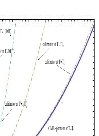
Figure 1: The normalized spectral intensities of CMB modes (thick line) at $T=T_{c}$ and $m_{\gamma}=0.1\,$GHz (in units of ordinary frequency) and of calibrator modes (dotted and dashed lines) at various temperatures. A null experiment asks for an intersection of the former with a representative of the one-parameter ($T$) familiy of the latter-type curves at a given frequency. Since for $y\to 0$ the Gaussian becomes stationary one has in this limit $T(y)=\mbox{const}\times y^{-2}$, that is, the asymptotic spectral index reads $\beta_{\tiny\mbox{as}}=-2$. With the low-frequency data presently available one has $\beta\sim-2.6$ [3].

For the extraction of $m_{\gamma}$ from the data let us introduce the following two dimensionless quantities

$$y\equiv\frac{\omega}{T_{c}}\,,\ \ \ \ \ \ \ \ \ \ \tau\equiv\frac{T}{T_{c}}\,.$$ (8)

With these definitions and appealing to Eqs. (6), (5), and (4), Eq. (7) is recast as

$$\tau=\sqrt{\frac{2}{\pi}}\,y^{-2}\,\exp\left(-\frac{y^{2}}{2\mu^{2}_{\gamma}}\right)\left(\frac{\mu_{\gamma}^{2}}{3}+\frac{F(\mu_{\gamma})}{\mu_{\gamma}}\right)+\theta(y-\mu_{\gamma})\frac{\sqrt{y^{2}-\mu_{\gamma}^{2}}}{\mbox{e}^{y}-1}\,.$$ (9)

The following table lists our results for $m_{\gamma}$, as extracted from the data using Eq. (9), in units of ordinary (not circular) frequency $\nu$:

$$\begin{array}[]{ccccc}\mbox{source}&\nu[\mbox{GHz}]&T[\mbox{K}]&\mu_{\gamma}&m_{\gamma}[\mbox{GHz}]\\ \hline\cr\mbox{Roger}&0.022&21200\pm 5125&0.001821^{+0.000423}_{-0.000419}&0.1034^{+0.0240}_{-0.0238}\\ \mbox{Maeda}&0.045&4355\pm 520&0.001704^{+0.000169}_{-0.000166}&0.0968^{+0.0095}_{-0.0095}\\ \mbox{Haslam}&0.408&16.24\pm 3.4&0.003611^{+0.000152}_{-0.000325}&0.205^{+0.0086}_{-0.0185}\\ \mbox{Reich}&1.42&3.213\pm 0.53&0.0093^{+0.0007}_{-0.00153}&0.528^{+0.0397}_{-0.0869}\\ \mbox{Arcade2}&3.20&2.792\pm 0.010&0.0211^{+0.0001}_{-0.0001}&1.198^{+0.0057}_{-0.0057}\\ \mbox{Arcade2}&3.41&2.771\pm 0.009&0.02253^{+0.0001}_{-0.0001}&1.279^{+0.0057}_{-0.0057}\end{array}$$

Notice the good agreement of $m_{\gamma}$ as extracted from the data of Roger [5] and Maeda [6] where $\nu<m_{\gamma}$. The other data of Haslam [7], Reich [8], and Arcade2 [3] yield $\nu>m_{\gamma}$ which is in the regime where we do not expect the spectral model for CMB photons to be good (average number of polarizations depends nontrivially on frequency). Still, the value of $m_{\gamma}$ obtained from Haslam’s data [7] is only twice as large as that arising from the data of Roger [5] or Maeda [6] at a frequency which is, respectively, twenty or ten times larger!

Meissner mass of $\sim 100\,$MHz? At this point it surely is worthwhile to discuss what it really means to have the thermalized photon field (at a temperature $T_{0}=2.727\,$K) acquire a Meissner mass? Is this scenario not ruled out by experiments such as radar vs. laser ranging to the moon and the limits on the photon mass obtained by terrestial Coulomb-law measurements or the measurement of the magnetic fields of astrophysical objects, see [15]. The answer is no for the following reason: Whether or not the propagation of the photon is altered as compared to conventional wisdom sensitively depends of the temperature of the thermal ensemble it belongs to and on its frequency. To be above the thermal noise of the CMB any experiment trying to detect a photon mass (either directly by looking for deviations in electrostatic or magnetostatic field configurations or indirectly by searching for modified dispersion laws in propagating photon fields) must work with local energy densities attributed to the photon field that are by many orders of magnitude larger than that of the CMB. Even though a static background field or laser emission or radar does not describe a homogeneous thermodynamical setting one may for a rough argument appeal to an adiabatic approximation setting the experimental energy density equal to that of thermal (deconfining) SU(2)${}_{\tiny\mbox{CMB}}$ to deduce the local temperature this energy density would correspond to were the experimental system actually thermalized. In any experimental circumstance searching for a universal (by assumption not dependent on temperature) photon mass this would yield a temperature far above $T_{0}=2.725\,$K. But we have shown in [14] how rapidly the thermalized SU(2) photon approaches U(1) behavior with increasing temperature by a power-like decrease of the modulus of its screening function. For example, the spectral gap $\omega^{*}/T$ in black-body spectra, defining the center of the spectral region where nonabelian effects are most pronounced (they decay exponentially for $\omega>\omega^{*}$) decays as $T^{-3/2}$. Thus systems that so far were used to obtain photon-mass bounds roughly would correspond to temperatures where the photon behaves in a purely abelian way explaining the very low mass bounds obtained. That is, for the photon to exhibit measurable deviations in its dispersion law it must belong to a thermal bath at temperatures from just below $T_{0}$ (Meissner mass) up to $10\,$K (momentum dependent screening mass), say.

What about the physics just around $T_{0}$? Is there a possibility that thermodynamics is not honoured? For example consider the following set-up. Two blackbodies (BBs), one at $T_{1}$ just below $T_{0}$, the other at $T_{2}$ just above $T_{0}$, are immersed into a photon bath exactly at temperature $T_{0}$. Photons exchanged by the two BBs are restricted to frequencies below $m_{\gamma}\sim 100\,$MHz. Would then not BB1 transfer energy to BB2 due to its larger spectral intensity below $m_{\gamma}$ – in contradiction to the second law of thermodynamics? The answer is no because the BB1 photons supporting this bump in the spectrum are evanescent and so, by definition, cannot propagate out of BB1’s cavity. Also, if $T_{0}<T_{1}<T_{2}$, and both $T_{1}$ and $T_{2}$ not too far above $T_{0}$ then the rapidly rising with temperature spectral intensity (in the Rayleigh-Jeans regime linearly) would assure, as it should, that BB1 warms up at the expense of BB2 despite the small spectral modifications (screening and antiscreening) at temperatures not far above $T_{0}$.
Discussion and Conclusions. Since we may not trust our spectral model for CMB modes locally if $\nu>m_{\gamma}$ (both expressed as ordinary frequencies) it is not surprising that considerable deviations occur for the extracted values of $m_{\gamma}$ compared to the low-frequency situation. The integral of the spectral model, which enters into the normalization $\Delta\rho$ of half the Gaussian in Eq. (5), however, is a quantity that is robust against local changes of the spectrum. Thus we are inclined to trust our result $m_{\gamma}\sim 0.1\,$GHz extracted at low frequencies (Roger, Maedan). Based on the present work two predictions, arising from an SU(2) Yang-Mills theory being responsible for photon propagation [11], can be made: First, since the low-frequency data on line temperatures are efficiently explained by this theory being at its deconfining-preconfining phase boundary one has $T_{c}=2.725\,$K. This allows for a precise prediction of a sizable anomaly in the low-frequency part of the thermal spectral intensity at higher, absolutely given temperatures, say at $T=2\,T_{c}\sim 5.4\,$K [13, 14]. Second, we predict that the spectral index $\beta$ for the line temperature $T(\nu)$, measured by nulling the CMB signal by a black-body reference load, approaches $\beta_{\tiny\mbox{as}}=-2$ for $\nu\searrow 0$. The tendency of increase of $\beta$ when fitting Eq. (1) to low-frequency as compared to intermediate frequency weighted data sets is nicely seen in Tab. 5 of [3].

The here presented strong indication that the CMB is on the verge of undergoing a phase transition towards superconductivity at its present baseline temperature $T_{\tiny\mbox{CMB}}=2.725\,$K implies radical consequences for particle physics [13]. Since this process occurs on a time scale of $\sim 2\,$ billion years [17] there is no immediate consequence for any form of energy consuming life.

References

-
[1]
D. J. Fixsen et al., Astrophys. J. 420, 457 (1994).
J. C. Mather et al., Astrophys. J. 420, 439 (1994).
J. C. Mather et al., Astrophys. J. Suppl. 170 288 (2007).
G. Hinshaw et al., astro-ph/0603451. -
[2]
A. Kogut et al., Astrophys. J. Suppl. 148, 161 (2003).
D. N. Spergel et al., Astrophys. J. Suppl. 148, 175 (2003).
D. N. Spergel et al., astro-ph/0603449.
L. Page et al., astro-ph/0603450.
G. Hinshaw et al., astro-ph/0603451.
N. Jarosik et al., astro-ph/0603452. - [3] D.J. Fixsen et al., arXiv:0901.0555.
- [4] M. Seiffert et al, arXiv:0901.0559.
- [5] R.S. Roger et al., A & AS, 137, 7 (1999).
- [6] Maeda et al., A & AS, 140, 145 (1999).
- [7] C.G.T. Haslam et al., A & A 100, 209 (1981).
- [8] Reich and Reich, A & AS, 63, 205 (1986).
-
[9]
A. de Oliveira-Costa, M. Tegmark, M. Zaldarriga, and A. Hamilton, Phys. Rev. D 69
063516 (2004). [arXiv:astro-ph/0307282]
D. J. Schwarz, G. D. Starkman, D. Huterer, and C. J. Copi, Phys. Rev. Lett. 93, 221301 (2004). [arXiv:astro-ph/0403353]
C. J. Copi, D. Huterer, D. J. Schwarz, and G. D. Starkman, Phys. Rev. D 75, 023507 (2007). [astro-ph/0605135]
C. J. Copi, D. Huterer, D. J. Schwarz, and G. D. Starkman, arXiv:0808.3767 [astro-ph].
P. Bielewicz, K. M. Gorski, and A. J. Banday, Mon. Not. Roy. Astron. Soc. 355, 1283 (2004). [arXiv:astro-ph/0405007] - [10] M. Szopa and R. Hofmann, JCAP 0803:001 (2008). [arXiv:hep-ph/0703119]
-
[11]
R. Hofmann, Int. J. Mod. Phys. A 20, 4123
(2005), Erratum-ibid. A 21, 6515 (2006). [arXiv:hep-th/0504064]
R. Hofmann, arXiv:0710.0962 [hep-th]. - [12] M. Schwarz, R. Hofmann, and F. Giacosa, Int. J. Mod. Phys. A 22, 1213 (2007). [arXiv:hep-th/0603078]
- [13] M. Schwarz, R. Hofmann, and F. Giacosa, JHEP 0702:091 (2007). [arXiv:hep-ph/0603174]
- [14] J. Ludescher and R. Hofmann, Ann. Phys. (Berlin) 18, 271 (2009). [arXiv:0806.0972 [hep-th]].
- [15] http://pdg.lbl.gov/2007/listings/s000.pdf.
- [16] J. Ludescher, J. Keller, F. Giacosa, and R. Hofmann, arXiv:0812.1858 [hep-th].
- [17] F. Giacosa and R. Hofmann, Eur. Phys. J. C 50, 635 (2007). [hep-th/0512184]