One-dimensional classical diffusion in a random force field
with weakly concentrated absorbers

Abstract

A one-dimensional model of classical diffusion in a random force field with a weak concentration $\rho$ of absorbers is studied. The force field is taken as a Gaussian white noise with $\left\langle\phi(x)\right\rangle=0$ and $\left\langle\phi(x)\phi(x^{\prime})\right\rangle=g\,\delta(x-x^{\prime})$. Our analysis relies on the relation between the Fokker-Planck operator and a quantum Hamiltonian in which absorption leads to breaking of supersymmetry. Using a Lifshits argument, it is shown that the average return probability is a power law $\langle P(x,t|x,0)\rangle\sim{}t^{-\sqrt{2\rho/g}}$ (to be compared with the usual Lifshits exponential decay $\exp{-(\rho^{2}t)^{1/3}}$ in the absence of the random force field). The localisation properties of the underlying quantum Hamiltonian are discussed as well.

1 Introduction

Classical diffusion in a random force field is encountered in several physical contexts of statistical physics related to anomalous diffusion or glassy dynamics due to the presence of disorder. As introduced by Sinai in the seminal work [1], it may be modelised via a Langevin equation $\dot{x}(t)=2\,\phi(x(t))+\sqrt{2}\,\eta(t)$, where $\phi(x)$ is a quenched random force field with short-range correlations, and $\eta(t)$ a Langevin force (a normalised Gaussian white noise). By now its large-time properties in one dimension are well understood : in the absence of a global drift, the random force leads to anomalous diffusion characterised by the scaling of the distance with time $x(t)\sim\ln^{2}t$. Normal diffusion properties are only recovered for a sufficiently large drift, however an intermediate regime reveals several interesting phases (see Ref. [2] for a review). Many approaches to this problem have been developed : a probabilistic method [2] (a continuous version of the Dyson-Schmidt method [3]), Berezinskii diagrammatic techniques [4, 5] as well the replica method [2]. Moreover more recently, interesting features of this model like aging properties were analyzed by means of Ma-Dasgupta real-space renormalisation group methods [6].

In this letter, we extend the analysis to random media containing randomly spread absorbers. Our approach relies on the Fokker-Planck equation (FPE)

$$\frac{\partial}{\partial t}P=\left(\frac{\partial^{2}}{\partial x^{2}}-2\frac{\partial}{\partial x}\phi(x)-A(x)\right)P\equiv-H_{\mathrm{FP}}P\>,$$ (1)

describing classical diffusion in a force field $\phi(x)$ in the presence of an absorber density $A(x)$. $P$ denotes the (conditional) probability $P(x,t|x^{\prime},0)$ to find a particle at $x$ at time $t$ which has started from $x^{\prime}$ at $t^{\prime}=0$. We consider the random force field to be $\phi(x)$ a Gaussian white noise of zero average $\left\langle\phi(x)\right\rangle=0$ and $\left\langle\phi(x)\phi(x^{\prime})\right\rangle=g\,\delta(x-x^{\prime})$ (throughout the paper, $\langle\cdots\rangle$ will denote averaging with respect to the quenched disorder : force field and absorbers). $A(x)$ describes absorbers at locations $x_{n}$ with annihilation rates $\alpha_{n}>0$, independently and uniformly distributed for a concentration $\rho$ ; thus we write $A(x)=\sum_{n}\alpha_{n}\,\delta(x-x_{n})$. The effects of the random force field and the random local annihilation rates are well known when described separately. Let us first review known results for the average return probability ($x=x^{\prime}$).

(i) $g=0$ & $\alpha=0$ : In the absence of random force fields and impurities, the conditional probability reads $P(x,t|x,0)=\frac{1}{\sqrt{4\pi\,t}}$.

(ii) $g\neq 0$ & $\alpha=0$ : For classical diffusion in a random force field (Sinai problem) [1, 2, 6], the decay is

$$\langle P(x,t|x,0)\rangle\underset{t\to\infty}{\sim}g\,\ln^{-2}(g^{2}t)\>,$$ (2)

and hence much slower than $1/\sqrt{t}$. This behaviour is related to the aforementioned typical distance $x(t)\sim g^{-1}\ln^{2}(g^{2}t)$.

(iii) $g=0$ & $\alpha\neq 0$ : For free diffusion with a weak absorber concentration we have

$$\langle P(x,t|x,0)\rangle\underset{t\to\infty}{\sim}\rho(\rho^{2}t)^{1/6}\,{\mbox{\large e}}^{-3(\frac{\pi}{2})^{2/3}(\rho^{2}t)^{1/3}}\>.$$ (3)

The rapid (exponential) decay is mostly explained by the decay of the survival probability $\int{\rm d}{}x\,\langle P(x,t|x^{\prime},0)\rangle\sim\exp-(\rho^{2}t)^{1/3}$ (probability is not conserved in the presence of absorption) (see [7] for a review on Lifshits tails). As switched on from free diffusion, the random force field strongly slows down the decay of the probability from $1/\sqrt{t}$ to $1/\ln^{2}t$, whereas absorbers tend to accelerate the decay from a power law to exponential $\exp{-t^{1/3}}$. The aim of the present paper is to study the interplay between the random force field and randomly dropped absorbers.

2 From FPE to Schrödinger equation

Our analysis relies on the well-known relation between the FPE (1) and the Schrödinger equation $-\partial_{t}\psi=H\psi$ for :

$$H=-\frac{{\rm d}^{2}}{{\rm d}x^{2}}+\phi(x)^{2}+\phi^{\prime}(x)+A(x)\equiv H_{\mathrm{susy}}+A(x)\>.$$ (4)

A mapping between the two equations is constructed via a non-unitary isospectral transformation $P(x,t)=\psi(x,t)\exp{\int^{x}\phi(x^{\prime}){\rm d}{x^{\prime}}}$. In the case $A=0$, this leads to the Hamiltonian $H_{\mathrm{susy}}=(\frac{{\rm d}}{{\rm d}x}+\phi)(-\frac{{\rm d}}{{\rm d}x}+\phi)$. This factorised, supersymmetric, structure is responsible for a positive spectrum. When $\phi$ is a white noise of zero mean, the spectrum presents a Dyson singularity at the band edge ($E=0$) [4, 8, 5, 2]. The presence of the absorption $A(x)$ in Hamiltonian (4) breaks the supersymmetry. Spectral and localisation properties of $H$ were investigated in Ref. [9] for the case of $A(x)$ and $\phi(x)$ both being white noises. This work focused on the mechanism leading to a (stochastic) supersymmetry breaking, giving rise to a lifting of the Dyson singularity and a breaking of the delocalisation transition at energy $E=0$. This first study is connected to the high density limit $\rho\gg\alpha_{n}$ of the model studied in the present paper. However Ref. [9] has led to the conclusion that the low density limit $\rho\ll\alpha_{n}$ studied below is more relevant in the context of classical diffusion.

In order to study diffusion properties via (4), let us recall that we may relate the return probability, averaged over the realisations of the random functions $\phi(x)$ and $A(x)$, to the Laplace transform of its density of states (DoS) :

$$\langle P(x,t|x,0)\rangle=\int{\rm d}E\,\rho(E)\,{\mbox{\large e}}^{-Et}\>.$$ (5)

Having this relation in mind, we now construct a Lifshits argument for the DoS $\rho(E)$ of the Hamiltonian (4).

2.1 Free diffusion with random absorbers ($g=0$ & $\alpha\neq 0$)

We first recall the famous Lifshits argument [10, 3] in the absence of the random force field $\phi\equiv 0$. Low-energy states are due to the formation of large impurity-free regions. Let us denote by $\ell$ the distance separating two neighboring impurities. For $1/\ell\sim\rho\ll\alpha_{n}$ they impose on the wave function to vanish at their location (indeed this holds rigorously for $\alpha_{n}\to\infty$) and the interval gives rise to a low-energy state $E_{1}\simeq(\pi/\ell)^{2}$. In terms of classical diffusion, the survival probability of a diffusive particle released in such an interval decays as ${\mbox{\large e}}^{-\pi^{2}t/\ell^{2}}$. Hence the probability for a low-energy state is related to the probability of a formation of a large interval : $\mathrm{Proba}[E_{1}<E]=\mathrm{Proba}[\ell>\pi/\sqrt{E}]$. Since the distribution of $\ell$ is $\rho\,{\mbox{\large e}}^{-\rho\ell}$ we recover the Lifshits singularity [10, 3] for the integrated density of states (IDoS) per unit length $N(E)\sim{\mbox{\large e}}^{-\pi\rho/\sqrt{E}}$. Using a steepest descent method, we can relate this low energy behaviour to the large time behaviour of $\langle P(x,t|x,0)\rangle$ and recover eq. (3) .

Let us work out a more precise argument : in the limit of high impurity weights, $\alpha_{n}\to\infty$, an interval of length $\ell_{i}$ between two impurities yields a contribution $\mathcal{N}_{0}(E;\ell_{i})=\sum_{n=1}^{\infty}\theta(E-(n\pi/\ell_{i})^{2})$ to the IDoS :

$$N(E)\underset{\rho\to 0}{\simeq}\lim_{M\to\infty}\frac{\sum_{i=1}^{M}\mathcal{N}_{0}(E;\ell_{i})}{\sum_{i=1}^{M}\ell_{i}}=\rho\,\left\langle\mathcal{N}_{0}(E;\ell)\right\rangle_{\ell}\>,$$ (6)

where the average is taken with respect to $\ell$ (this approximation corresponds to the “pieces model” of Ref. [12, 3]). We have $N(E)=\rho\sum_{n=1}^{\infty}\int_{n\pi/\sqrt{E}}^{\infty}{\rm d}\ell\,\rho\,e^{-\rho\ell}$ what yields [13]

$$N(E)\simeq\frac{\rho}{{\mbox{\large e}}^{\pi\rho/\sqrt{E}}-1}\>\hskip 14.22636pt\mbox{for }\sqrt{E},\,\rho\ll\alpha.$$ (7)

2.2 Random force field with absorbers ($g\neq 0$ & $\alpha\neq 0$)

We now apply the same argument to the Hamiltonian (4) in order to obtain the low energy DoS. Due to the supersymmetric potential $\phi(x)^{2}+\phi^{\prime}(x)$, the energy levels $E_{n}$ associated to an interval of length $\ell$ differ from $(n\pi/\ell)^{2}$, and rather are distributed according to some nontrivial laws $W_{n}(E;\ell)$ obtained in Ref. [14]. Similarly to (6), we have

$$N(E)\underset{\rho\to 0}{\simeq}\rho\,\langle\mathcal{N}_{\mathrm{susy}}(E;\ell)\rangle_{\ell}\>,$$ (8)

where $\mathcal{N}_{\mathrm{susy}}(E;\ell)$ is the IDoS of $H_{\mathrm{susy}}$ on $[0,\ell]$ for Dirichlet boundary conditions. We use the decomposition over the distributions of eigenvalues $\mathcal{N}_{\mathrm{susy}}(E;\ell)=\sum_{n=1}^{\infty}\int_{0}^{E}{\rm d}E^{\prime}\,W_{n}(E^{\prime};\ell)$. Following  [14], in the limit $g\ell\gg 1$ and for $E\ll{}g^{2}$, we may write the distribution of the $n$-th energy level as $W_{n}(E;\ell)\simeq\ell\,N^{\prime}_{\mathrm{susy}}(E)\,\varpi_{n}(\ell\,N_{\mathrm{susy}}(E))$, where $N_{\mathrm{susy}}(E)=\lim_{\ell\to\infty}\frac{1}{\ell}\mathcal{N}_{\mathrm{susy}}(E;\ell)=\frac{2g/\pi^{2}}{J_{0}(\sqrt{E}/g)^{2}+N_{0}(\sqrt{E}/g)^{2}}$ [8, 2] is the IDoS per unit length for an infinite volume ; $J_{0}(x)$ and $N_{0}(x)$ are the Bessel functions of first and second kind, respectively. Contrary to $\mathcal{N}_{\mathrm{susy}}(E;\ell)$, the IDoS per unit length $N_{\mathrm{susy}}(E)$ is insensitive to boundary effects. Finally

$$N(E)\underset{\rho\to 0}{\simeq}\rho\,\int_{0}^{\infty}{\rm d}\ell\,\rho\,{\mbox{\large e}}^{-\rho\ell}\sum_{n=1}^{\infty}\int_{0}^{\ell N_{\mathrm{susy}}(E)}{\rm d}x\,\varpi_{n}(x)\>.$$ (9)

We use the integral representation [14] $\varpi_{n}(x)=\int_{\mathcal{B}}\frac{{\rm d}{}q}{2{\rm i}\pi}\,\frac{e^{qx}}{\cosh^{2n}\sqrt{q}}$, where $\mathcal{B}$ is a Bromwich contour (axis going from $c-{\rm i}\infty$ to $c+{\rm i}\infty$ with all singularities of the integrand at its left), and obtain :

$$N(E)\simeq\rho\int_{0}^{\infty}{\rm d}\ell\,\rho\,{\mbox{\large e}}^{-\rho\ell}\sum_{n=1}^{\infty}\int_{\mathcal{B}}\frac{{\rm d}q}{2{\rm i}\pi}\,\frac{{\mbox{\large e}}^{q\ell N_{\mathrm{susy}}(E)}-1}{q\,\cosh^{2n}\sqrt{q}}\>.$$ (10)

If we permute order of integrations, perfom the integral with respect to $\ell$ and the summation we find

$$N(E)\simeq\rho\int_{\mathcal{B}}\frac{{\rm d}q}{2{\rm i}\pi}\,\frac{1}{\rho/N_{\mathrm{susy}}(E)-q}\,\frac{1}{\sinh^{2}\sqrt{q}}\>.$$ (11)

Notice that this procedure only converges for a Bromwich contour with $0<c<q_{\ast}=\rho/N_{\mathrm{susy}}(E)$, what always can be attained via a suitable contour deformation. Applying the residue theorem to the simple pole at $q_{\ast}$, we obtain our main result for the low energy IDoS per unit length

$$\boxed{N(E)\simeq\frac{\rho}{\sinh^{2}\sqrt{\rho/N_{\mathrm{susy}}(E)}}}\hskip 14.22636pt\mbox{for }E\ll g^{2},\>\alpha^{2}\>.$$ (12)

The aforementioned condition $g\ell\gg 1$, where $\ell$ denotes the length of an interval, turns out to be a low density condition $\rho\ll{}g$ under which (12) is valid. For completeness, note that $E\gg g^{2},\,\alpha^{2}$ corresponds to the perturbative regime where we recover the free IDoS $N(E)\simeq\frac{1}{\pi}\sqrt{E}$. Eq. (12) allows to identify the energy scale $E_{c}=g^{2}{\mbox{\large e}}^{-\sqrt{2g/\rho}}$ separating two regimes. In the intermediate energy range, $E_{c}\ll E\ll g^{2}$, we recover the IDoS of $H_{\mathrm{susy}}$

$$N(E)\simeq N_{\mathrm{susy}}(E)\simeq\frac{2g}{\ln^{2}(g^{2}/E)}\>.$$ (13)

It is only in the narrow region $0<E\lesssim E_{c}$ that the scalar potential $A(x)$ affects the spectrum, for $E\ll{}E_{c}$ :

$$\boxed{N(E)\underset{\rho\to 0}{\simeq}4\rho\,\left(\frac{E}{g^{2}}\right)^{\sqrt{2\rho/g}}}\>.$$ (14)

Interestingly, we notice that this power law behaviour stems from the ground state energy $E_{1}$ of each interval between consecutive impurities. Indeed, we may check that eq. (14) can be obtained from $N(E)\simeq\rho\langle\theta(E-E_{1}[\phi(x),\ell])\rangle_{\phi,\,\ell}$, by means of the distribution $W_{1}(E;\ell)$, involving $\varpi_{1}(x)=\frac{4}{\sqrt{\pi}\,x^{3/2}}\sum_{m=1}^{\infty}(-1)^{m+1}m^{2}{\mbox{\large e}}^{-m^{2}/x}$ [14]. A priori it is far from being obvious that the analysis can be restricted to the ground state of each interval since the distributions $W_{n}(E;\ell)$ have strong overlaps [14].

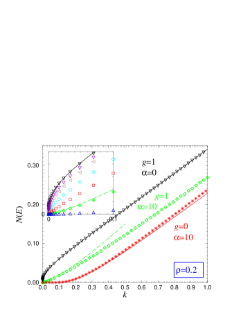
Figure 1: Comparison between numerical results (triangles, diamonds & stars) and analytical results (lines). Inset : IDoS for $g=1$ with $\rho$ ranging from $0.01$ to $0.5$.

Again, combining (14) and a steepest descent argument for (5), we relate the power law behaviour of the IDoS to a power law decay of the particle density for $t\gg\frac{1}{g^{2}}{\mbox{\large e}}^{\sqrt{2g/\rho}}$

$$\boxed{\langle P(x,t\to\infty|x,0)\rangle\underset{\rho\to 0}{\simeq}\frac{4\rho\,\Gamma(\sqrt{2\rho/g}+1)}{(g^{2}t)^{\sqrt{2\rho/g}}}}\>.$$ (15)

The crossover time scale $t_{c}=g^{-2}\exp{\sqrt{2g/\rho}}$ corresponds to the time needed by the random particle released in the random force field to reach the nearest absorber : $x(t_{c})\sim 1/\rho$ where $x(t)\sim{}g^{-1}\ln^{2}(g^{2}t)$. The return probability (15) decays faster than (2) but slower than the exponential decay (3) in the absence of the random force field. This provides the answer to our initial question.

3 Localisation

We now analyse the localisation properties of the underlying quantum Hamiltonian (4).

(i) $g\neq 0$ & $\alpha=0$ : In the absence of absorption, $A(x)=0$, the Lyapunov exponent (inverse localisation length) is exactly known [2] $\gamma_{\mathrm{susy}}(E)=-\frac{g}{2}k\frac{{\rm d}}{{\rm d}{}k}\ln[J_{0}^{2}(k/g)+N_{0}^{2}(k/g)]$. It reaches a finite value at high energy $\gamma_{\mathrm{susy}}(E\gg{}g^{2})\simeq{}g/2$ and vanishes at zero energy :

$$\gamma_{\mathrm{susy}}(E\to 0)\simeq\frac{g}{\ln(g/k)}\to 0\>.$$ (16)

(ii) $g=0$ & $\alpha\neq 0$ : On the other hand, in the absence of supersymmetric noise, $\phi(x)=0$, and for a low density of impurities, $\rho\ll\alpha$, the Lyapunov exponent is given by $\gamma_{\mathrm{scalar}}(E)\simeq\frac{\rho}{2}\ln[1+(\frac{\alpha}{2k})^{2}]$ for $k\gg\rho$ [3, 15]. At high energy it leads to the well known linear increase of the localisation length as a function of the energy [16] $1/\ell_{\mathrm{loc}}=\gamma_{\mathrm{scalar}}(E)\simeq\rho\alpha^{2}/(8E)$ for $E\to\infty$. At zero energy it reaches a finite value given by [3, 17]

$$\gamma_{\mathrm{scalar}}(E=0)\simeq\rho\,[\ln(\alpha/\rho)-\mathrm{C}]\hskip 14.22636pt\mbox{for }\rho\ll\alpha\>,$$ (17)

where $\mathrm{C}\simeq 0.577$ is the Euler constant.

(iii) $g\neq 0$ & $\alpha\neq 0$ : We now turn to the case where $\phi$ and $A$ both differ from zero. The high energy (perturbative) expression is : $\gamma(E)\simeq\frac{\rho\alpha^{2}}{8E}+\frac{g}{2}$. It corresponds to the addition of the perturbative expressions for $\gamma_{\mathrm{scalar}}(E)$ and $\gamma_{\mathrm{susy}}(E)$ (a similar result was obtained in Ref. [9] when $A$ is a Gaussian white noise). We can see on figure 2 that, for a fixed $g$, $\gamma(E)$ (obtained numerically) slowly converges to $\gamma_{\mathrm{susy}}(E)$ as $\rho$ is decreased. The introduction of the scalar potential $A(x)$ breaks the delocalisation at $E=0$ obtained for the supersymmetric Hamiltonian.

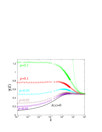
Figure 2: Low energy Lyapunov exponent as a function of energy for $\rho$ ranging from $0.2$ to $0.01$ ; with $g=1$. Black line : $\gamma_{\mathrm{susy}}(E)$. Green dashed line : perturbative result for $\rho=0.2$.

Let us now turn to the detailed analysis of the zero energy Lyapunov exponent. For this purpose it is convenient to convert the Schrödinger equation $H\psi=E\psi$ into a stochastic differential equation for the Ricatti variable $z=\psi^{\prime}/\psi-\phi$ : this latter obeys $\frac{\mathrm{d}}{\mathrm{d}x}z=-E-z^{2}-2z\,\phi(x)+A(x)$. This Langevin like equation can be related to a Fokker-Planck type equation for the distribution $\partial_{x}T(z;x)=\partial_{z}[(E+z^{2})T(z;x)]+2g\partial_{z}\big{[}z\partial_{z}[zT(z;x)]\big{]}+\rho[T(z-\alpha;x)-T(z;x)]$, where the first term is a drift term related to the force field $F(z)=-E-z^{2}$, the second term a diffusive term and the last term is a jump term originating from the scalar impurities $A(x)$. For $E>0$ the Ricatti variable is driven from $+\infty$ to $-\infty$ in a finite “time” $x$. The steady current of $z(x)$ corresponds to its number of divergences per unit length, i.e. the number of nodes of the wave function $\psi$ per unit length, that is to $N(E)$. The distribution reaches a stationary distribution $T(z;x\to\infty)=T(z)$ for a steady current $-N(E)$ :

$$N(E)=(E+z^{2})T(z)+2gz\frac{\mathrm{d}}{\mathrm{d}z}[zT(z)]-\rho\int_{z-\alpha}^{z}{\rm d}z^{\prime}\,T(z^{\prime})$$ (18)

The IDoS is given by normalising the solution of this integral equation. Given $T(z)$, the IDoS can be extracted from the distribution thanks to the Rice formula $N(E)=\lim_{z\to\infty}z^{2}T(z)$. Lyapunov exponent is given by [3] $\gamma(E)=\langle z\rangle=\lim_{R\to\infty}\int_{-R}^{+R}{\rm d}{z}\,z\,T(z)$.

For $E=0$ and positive jumps $\alpha>0$, the Ricatti is constrained to belong to ${\ensmathonze R}^{+}$ since both the “force” $F(z)$ and the effect of the multiplicative noise $\phi(x)$ vanish for $z=0$ : we recover $N(E=0)=0$. In the low density limit $\rho\to 0$ the Ricatti variable is driven to $z\sim 0$ and eventually reinjected at $z\sim\alpha$ with a “rate” $\rho$. We can write that the negative current due to the “force” $F(z)$ and the noise $\phi(x)$ is equilibrated by the positive current $\rho$ due to the jumps : $\rho\simeq{}z^{2}T(z)+2gz\frac{\mathrm{d}}{\mathrm{d}z}[zT(z)]$ for $z\in[z_{c},\alpha]$. We have introduced a cutoff $z_{c}$ where the jump occur almost surely (the force $F(z)$ and the multiplicative noise vanish effectively as $z\to 0$). The solution of this equation is $T(z)\underset{\rho\to 0}{\simeq}\frac{\rho}{2g}\frac{1}{z}{\mbox{\large e}}^{-z/2g}\int_{z_{c}}^{z}\frac{{\rm d}z^{\prime}}{z^{\prime}}{\mbox{\large e}}^{z^{\prime}/2g}$. This distribution may be approximated by $T(z)\simeq\frac{\rho}{2gz}\ln(z/z_{c})$ for $z_{c}\lesssim{z}\lesssim{g}$ and $T(z)\simeq\frac{\rho}{z^{2}}$ for $g\lesssim{z}\lesssim\alpha$ (and $T(z)\simeq 0$ elsewhere). Normalisation gives $\ln^{2}(g/z_{c})\simeq\frac{4g}{\rho}$. Using $\gamma=\left\langle z\right\rangle$, we get

$$\boxed{\gamma(0)\underset{\rho\to 0}{\simeq}\sqrt{\rho g}+\rho\ln(\alpha/g)}\>.$$ (19)

The second term is reminiscent of the result obtained in the absence of the supersymmetric noise. However the dominant term involves a nontrivial combination of $\rho$ and $g$. In the region of rarefaction of eigenstates ($E\sim 0$), the localisation length reads $\ell_{\mathrm{loc}}=1/\gamma\sim\frac{1}{\rho}\sqrt{\rho/g}\ll 1/\rho$. The scalar impurities breaks the delocalisation transition of the supersymmetric Hamiltonian, but quite surprisingly the localisation length is much smaller than the inverse density of impurities.

4 Numerics

We now turn to a numerical analysis in order to check our analytical results for spectrum and localisation and explore more precisely their validity range. We analyse the Hamiltonian (4) for $\phi(x)=\sum_{n}\lambda_{n}\delta(x-x_{n})$ and $A(x)=\sum_{n}\alpha_{n}\delta(x-x_{n})$. This choice of modelisation of the random force field $\phi$ allows to deal with a continuous description. The locations $x_{n}$ are uniformly distributed and uncorrelated, with densities $\rho_{\phi}$ for those of $\phi(x)$ and $\rho$ for impurities of $A(x)$. The precise shape of the distribution for the dimensionless weights $\lambda_{n}$ is not important, as long as it satisfies $\left\langle\lambda_{n}\right\rangle=0$ and $\langle\lambda_{n}^{2}\rangle$ finite. We choose a symmetric exponential law $p(\lambda_{n})=\frac{1}{2\lambda}{\mbox{\large e}}^{-|\lambda_{n}|/\lambda}$. The process $\phi(x)$ behaves as a Gaussian white noise in the limit $\rho_{\phi}\to\infty$ and $\lambda\to 0$, with $g=\rho_{\phi}\langle\lambda_{n}^{2}\rangle=2\rho_{\phi}\lambda^{2}$ fixed.

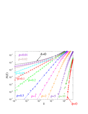
Figure 3: Dashed lines correspond to $N(E)\propto{E}^{\sqrt{2\rho/g}}$. Impurity weight is $\alpha=50$ and the number of impurities is $N_{i}=10^{7}$ ($N_{i}=10^{8}$ for the largest densities and smallest energies). The red line is eq. (7) and the red stars are the corresponding numerical calculation, for $\rho=10$.

4.1 Phase formalism

Let us now explain how we can obtain the spectral density from the phase formalism [16, 3]. In the equation $H\psi=E\psi$, we replace the couple of variables $(\psi,\psi^{\prime})$ by the couple $(\theta,\xi)$ defined as $\psi={\mbox{\large e}}^{\xi}\sin\theta$ and $\psi^{\prime}-\phi\psi=k{\mbox{\large e}}^{\xi}\cos\theta$, where $E=k^{2}$. The two variables obey the differential equations [9] :

$$\frac{{\rm d}\theta}{{\rm d}x} = k-\frac{A(x)}{k}\sin^{2}\theta+\phi(x)\,\sin 2\theta$$ (20)

$$\frac{{\rm d}\xi}{{\rm d}x} = \frac{A(x)}{2k}\sin 2\theta-\phi(x)\,\cos 2\theta$$ (21)

We solve these equations as follows

• We denote $\ell_{n}=x_{n+1}-x_{n}$. The evolution of the variables on an interval free of impurity is $\theta_{n+1}^{-}-\theta_{n}^{+}=k\ell_{n}$ and $\xi_{n+1}^{-}-\xi_{n}^{+}=0$, where $\theta_{n}^{\pm}\equiv\theta(x_{n}^{\pm})$ and $\xi_{n}^{\pm}\equiv\xi(x_{n}^{\pm})$ are values just before ($-$) or right after ($+$) the $n$-th impurity. The size of these intervals is distributed according to the Poisson law $P(\ell)=\rho_{\mathrm{tot}}{\mbox{\large e}}^{-\rho_{\mathrm{tot}}\ell}$ for a density $\rho_{\mathrm{tot}}=\rho+\rho_{\phi}$.

• The effect of a $\delta$-peak of $A(x)$ is given by $\mathop{\mathrm{cotg}}\nolimits\theta_{n}^{+}-\mathop{\mathrm{cotg}}\nolimits\theta_{n}^{-}=\frac{\alpha_{n}}{k}$ and $\xi_{n}^{+}-\xi_{n}^{-}=\ln\frac{\sin\theta_{n}^{-}}{\sin\theta_{n}^{+}}=\frac{1}{2}\ln\big{[}1+\frac{\alpha_{n}}{k}\sin 2\theta_{n}^{-}+\frac{\alpha_{n}^{2}}{k^{2}}\sin^{2}\theta_{n}^{-}\big{]}$ (see Ref. [17]).

• The effect of a $\delta$-peak of $\phi(x)$ is given by $\tan\theta_{n}^{+}=\tan\theta_{n}^{-}\,{\mbox{\large e}}^{2\lambda_{n}}$ and $\xi_{n}^{+}-\xi_{n}^{-}=\frac{1}{2}\ln\frac{\sin 2\theta_{n}^{-}}{\sin 2\theta_{n}^{+}}=\frac{1}{2}\ln\big{[}{\mbox{\large e}}^{2\lambda_{n}}\sin^{2}\theta_{n}^{-}+{\mbox{\large e}}^{-2\lambda_{n}}\cos^{2}\theta_{n}^{-}\big{]}$ (see Ref. [15]).

It is worth noticing that the two effects on the envelope of the wave function are roughly given by $\Delta\xi_{n}=\xi_{n}^{+}-\xi_{n}^{-}\sim\ln\alpha_{n}$ and $\Delta\xi_{n}\sim|\lambda_{n}|$.

The IDoS corresponds to the number of zeros of the wavefunction of energy $E$, i.e. the number of times the cumulative phase $\theta(x)$ coincides with an integer multiple of $\pi$. Therefore, a convenient way to get the IDoS numerically is [16, 3] $N(E)=\lim_{x\to\infty}\frac{\theta(x)}{\pi\,x}$. Moreover, the damping of the envelope is characterised by the Lyapunov exponent $\gamma(E)=\lim_{x\to\infty}\frac{\xi(x)}{x}$, providing a definition of the inverse localisation length ($\ell_{\mathrm{loc}}=1/\gamma$).

4.2 Ricatti variable

The equations of the phase formalism are singular in the limit $E\to 0$. In order to obtain the zero energy Lyapunov exponent, it is more simple to perform the analysis in term of the Ricatti variable. Let us denote $z_{n}^{\pm}=z(x_{n}^{\pm})$ its values before/after the impurity $n$. Between two impurities the evolution is given by $\arctan\big{(}{z_{n+1}^{-}}/{k}\big{)}-\arctan\big{(}{z_{n}^{+}}/{k}\big{)}=-k\ell_{n}$, i.e. $1/{z_{n+1}^{-}}-1/{z_{n}^{+}}=\ell_{n}$ for $E=0$. Through a scalar impurity of $A(x)$ we have $z_{n}^{+}-z_{n}^{-}=\alpha_{n}$ and through an impurity of $\phi(x)$ we have $z_{n}^{+}=z_{n}^{-}\,{\mbox{\large e}}^{-2\lambda_{n}}$. IDoS and Lyapunov exponent can be extracted from the stationary distribution of the Ricatti as explained above.

4.3 Results

As a first check, we consider the case with $\phi\equiv 0$ : we compare numerics for $\lambda=0$ to the Lifshits singularity (7) (red stars and red line on figure 1) and obtain a good agreement (some deviations appear for larger $k$ since $N(E\gg\alpha^{2})\simeq\frac{\sqrt{E}}{\pi}$). Next, we treat the case with $A=0$ and check the numerics (black triangles on figure 1) against the analytical expression recalled above [8, 2] (black continuous line) $N_{\mathrm{susy}}(E\to 0)=\frac{g/2}{[\ln(2g/k)-\mathrm{C}]^{2}+\pi^{2}/4}+O\big{(}\frac{k^{2}}{\ln^{2}k}\big{)}$. The agreement to the theory shows that our modelisation of Gaussian white noise $\phi$ is adequate.

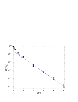
Figure 4: Numerical result for function $B(x)$. Lines are purely indicative (they correspond to ${\mbox{\large e}}^{-4x}$ and ${\mbox{\large e}}^{-2x}/4$).

Finally, we combine both noises (green diamonds on Fig. 1 and inset), and check against the power law $N(E\to 0)\propto{}E^{\sqrt{2\rho/g}}$ : the exponent fits very well within a surprisingly wide range (see figure 3 for densities ranging from $\rho=0.01$ to $5$). We insist that slopes in the log-log plot are not fitted but directly compared to $\sqrt{2\rho/g}$ (straight dashed lines). We however observe that, apart for the lowest densities, the prefactor significantly differs from $4\rho$, eq. (14). Since the IDoS reaches a finite limit for $\alpha\to\infty$, the additional dimensionless factor is a function of the ratio $\rho/g$ only. We conclude that numerics suggests the form $N(E\to 0)\simeq 4\rho\,B(\rho/g)\,\big{(}\frac{E}{g^{2}}\big{)}^{\sqrt{2\rho/g}}$ with $B(x\to 0)=1$. The function $B(x)$ is extracted from numerics and plotted on figure 4. For $\rho/g=10$, the numerical precision does not allow a convincing fit for the lowest energies (green diamonds of Fig. 3). We have however checked that the noise $\phi(x)$ still affects the IDoS which has not yet reached the Lifshits result (7) (red stars and line).

The energy dependence of the Lyapunov exponent is obtained from the phase formalism. The results are plotted for different densities $\rho$ on figure 2. In a second step we analyze the dynamic of the Ricatti variable for $E=0$. The stationary distribution is plotted on the inset of figure 5 on which we can check the crossover between the behaviours $T(z)\propto 1/z$ and $T(z)\propto 1/z^{2}$ occuring for $z\sim{g}=1$ (note however that prefactors do not fit with the one derived above). The distribution is used to compute the zero energy Lyapunov exponent. The analytical result (19) is compared to the numerical result and satisfactory coincides (Fig. 5).

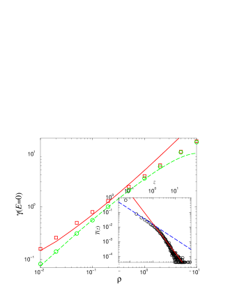
Figure 5: Lyapunov exponent at $E=0$. Green dashed line : in the absence of supersymmetric noise, for $\alpha=50$. Numerics (circles) is compared to equation (17). Red : with $\phi(x)$ ($g=1$). Comparison with expression (19). Inset : Stationary distribution of the Ricatti variable in this latter case ($\rho=0.05$) ; dashed blue line is $\propto 1/z$ and red line $\propto 1/z^{2}$.

5 Conclusion

We have studied the average return probability for one-dimensional classical diffusion in a random force field and the presence of absorbers at weak concentration ($\rho\to 0$), yet with strong absorption rates. We have shown that absorption only takes place above a very large time scale $t_{c}=g^{-2}{\mbox{\large e}}^{\sqrt{2g/\rho}}$. The well-known Sinai decay $\langle P(x,t|x,0)\rangle\simeq{2g}\,{\ln^{-2}(g^{2}t)}$ holds for $t\ll{t_{c}}$ and is replaced by the power law $\langle P(x,t|x,0)\rangle\simeq{4\rho}\,{(g^{2}t)^{-\sqrt{2\rho/g}}}$ for $t\gg{t_{c}}$. Whereas a simple guess would have been to put the crossover between (3) and (15) at $g\sim\rho$, the power law (15) persists numerically up to large ratio $\rho/g$. It would be interesting to understand more carefully the crossover and obtain analytically the prefactor $B(\rho/g)$ not predicted in our calculation. Another interesting issue would be to investigate the fluctuations of the return probability $P(x,t|x,0)$ over disorder configurations ; such a question is related to the characterisation of the fluctuations of the local DoS of the quantum Hamiltonian, a question studied for high energies for the scalar noise in Ref. [18] and for the supersymmetric noise in Ref. [19].

The localisation properties of the underlying quantum Hamiltonian have been considered, too. In particular, the scalar impurities lifts the divergence of the localisation length (inverse Lyapunov exponent) at energy $E=0$ and leads to a localisation length $\ell_{\mathrm{loc}}\sim 1/\sqrt{g\rho}$ for $\rho\to 0$.

References

- [1] Ya. G. Sinai, The limit behavior of random walks in a one-dimensional random environment, Theory of Prob. and Appl. 27(2), 247 (1982).
- [2] J.-P. Bouchaud, A. Comtet, A. Georges, and P. Le Doussal, Classical diffusion of a particle in a one-dimensional random force field, Ann. Phys. (N.Y.) 201, 285 (1990).
- [3] I. M. Lifshits, S. A. Gredeskul, and L. A. Pastur, Introduction to the theory of disordered systems, John Wiley & Sons, 1988.
- [4] A. A. Gogolin and V. I. Mel’nikov, Conductivity of one-dimensional metal with half-filled band, Sov. Phys. JETP 46, 369 (1977).
- [5] A. A. Gogolin, Electron localization and hopping conductivity in one-dimensional disordered systems, Phys. Rep. 86(1), 1 (1982).
- [6] P. Le Doussal, C. Monthus, and D. S. Fisher, Random walkers in one-dimensional random environments: Exact renormalization group analysis, Phys. Rev. E 59(5), 4795 (1999).
- [7] J.-M. Luck, Systèmes désordonnés unidimensionnels, CEA, collection Aléa Saclay, Saclay, 1992.
- [8] A. A. Ovchinnikov and N. S. Erikmann, Density of states in a one-dimensional random potential, Sov. Phys. JETP 46, 340 (1977).
- [9] C. Hagendorf and C. Texier, Breaking supersymmetry in a one-dimensional random Hamiltonian, J. Phys. A: Math. Theor. 41, 405302 (2008).
- [10] I. M. Lifshits, Energy spectrum structure and quantum states of disordered condensed systems, Sov. Phys. Usp. 18(4), 549 (1965).
- [11] R. Friedberg and J. M. Luttinger, Density of electronic energy levels in disordered systems, Phys. Rev. B 12(10), 4460 (1975).
- [12] L. N. Grenkova, S. A. Molčanov, and J. N. Sudarev, On the Basic States of One-Dimensional Disordered Structures, Commun. Math. Phys. 90, 101 (1983).
- [13] Yu. A. Bychkov and A. M. Dykhne, Electron spectrum in a one-dimensional system with randomly arranged scattering centers, Pis’ma Zh. Eksp. Teor. Fiz. 3(8), 313 (1966).
- [14] C. Texier, Individual energy level distributions for one-dimensional diagonal and off-diagonal disorder, J. Phys. A: Math. Gen. 33, 6095 (2000).
- [15] T. Bienaimé and C. Texier, Localization for one-dimensional random potentials with large fluctuations, J. Phys. A: Math. Theor. 41, 475001 (2008).
- [16] T. N. Antsygina, L. A. Pastur, and V. A. Slyusarev, Localization of states and kinetic properties of one-dimensional disordered systems, Sov. J. Low Temp. Phys. 7(1), 1 (1981).
- [17] C. Texier, Quelques aspects du transport quantique dans les systèmes désordonnés de basse dimension, PhD thesis, Université Paris 6, 1999, available at http://www.lptms.u-psud.fr/membres/texier/research.html.
- [18] B. L. Altshuler and V. N. Prigodin, Distribution of local density of states and NMR line shape in a one-dimensional disordered conductor, Sov. Phys. JETP 68(1), 198 (1989).
- [19] J. E. Bunder and R. H. McKenzie, Derivation of the probability distribution function for the local density of states of a disordered quantum wire via the replica trick and supersymmetry, Nucl. Phys. B [FS] 592, 445 (2001).