Robustness of geometric phase under parametric noise

Abstract

We study the robustness of geometric phase in the presence of parametric noise. For that purpose we consider a simple case study, namely a semiclassical particle which moves adiabatically along a closed loop in a static magnetic field acquiring the Dirac phase. Parametric noise comes from the interaction with a classical environment which adds a Brownian component to the path followed by the particle. After defining a gauge invariant Dirac phase, we discuss the first and second moments of the distribution of the Dirac phase angle coming from the noisy trajectory.

PACS: 03.65.Vf, 02.50.Ey, 03.67.-a

1 Introduction

The first reference to the role played by geometric phases in physics dates back to the work of S. Pancharatnam [1] in the context of interferometry of polarized beams of light. Later the same phenomenon was described by M. V. Berry [2] for quantum mechanical systems in the adiabatic limit. A mathematical insight into its origin was provided by B. Simon [3] which recognized that Berry phases could be interpreted as holonomies on a fiber bundle. Subsequently, quantum geometric phases (i.e. quantum holonomies) have been predicted and observed in various physical systems, and several generalizations and extensions were proposed [4, 5, 6] (see [7] and the references therein). Generally speaking, we may say that geometric phases appear in correspondence with a cyclic evolution of a relevant Hilbert (sub)space. The dimension of the cyclic (sub)space determines the features of the corresponding geometric phase: Abelian, i.e. $\mathrm{U}(1)$-valued, for Hilbert space of unit dimension, nonAbelian, i.e. $\mathrm{U}(N)$-valued, in the case of $N$-dimensional cyclic Hilbert space.

Few years after the seminal papers by M. V. Berry and B. Simon, the scientific community discovered the potentialities of quantum mechanical systems in the context of information and communication technology [8], leading to the birth of quantum information science [9]. Since information processing obeys physical laws, a reversible quantum algorithm is represented by a unitary transformation as long as information is encoded as vectors in a Hilbert space. It follows that quantum holonomies, being unitary transformations, can serve as quantum logical gates to implement quantum algorithms. This idea was first proposed and discussed in [10], where the authors also proved that universal computation [11] can be in general realized by means of solely (nonAbelian) geometric phases. A vast literature followed, which included both theoretical proposals [12, 13] and experimental realizations [14, 15] of simple holonomic quantum gates.

In view of the application for quantum information processing, one usually considers the case of adiabatic geometric phase (also called Berry phase). In this case the system Hamiltonian is supposed to be a smooth function of the coordinates on a suitable manifold, often called the ‘parameter manifold’. The geometric phase arises in the adiabatic approximation in correspondence with a closed loop in the parameter manifold.

It is worth remarking, however, that that geometric approach to the computation can be rather demanding from a technological point of view. Nevertheless, its advantage with respect to the standard dynamical approaches relies on the fact that Berry phases are argued to be particular robust with respect to noise. In particular, it is argued that holonomic quantum gates can be robust with respect to certain kind of classical parametric noise [16]. This kind of noise can be modeled as coming from the interaction with a classical environment.

The robustness of quantum logic gates is indeed a crucial issue because of the inherent fragility of quantum mechanical systems. Hence, although quantum error correction protocols exist [17], quantum gates which are a priori robust are welcome. It is worthwhile to mention another remarkable proposal for a fault tolerant computation, namely topological computation [18]. This approach is based on nonAbelian Aharonov-Bohm topological phases.

As we have anticipated, the geometric phase is believed to be robust with respect to classical parametric noise. This argument has been the central issue of several investigations, in particular we mention the work by the G. De Chiara and M. G. Palma [19], as well as the results presented in [20]. Several physical models have been taken into consideration to the study of the robustness of geometric phase. Recently, the robustness of geometric phase has been tested experimentally in trapped polarized ultra-cold neutrons [21]. However it is worth noticing that this issue is largely independent of the details of the physical model under consideration. For this reason, our discussion will be devoted to the simplest settings in which geometric phases appear. In the following sections we consider a charged semiclassical particle which is adiabatically and cyclically moved in a static magnetic field. The particle acquires the Dirac phase which is proportional to the magnetic flux enclosed by the particle trajectory. Two different settings will be described: in the first case the semiclassical particle is in the presence of a homogeneous magnetic field; in the second example the particle is subject to the field generated by a magnetic monopole.

2 Dirac phase under noise

In the following sections we consider the effects of parametric noise on quantum holonomies in two simple but remarkable examples. We consider as well two models for the noise, respectively represented by a Wiener and by a Ornstein-Uhlenbeck process. The examples involve a simple physical system made of a charged semiclassical particle in the presence of a static magnetic field $\mathbf{B}\equiv(B_{x},B_{y},B_{z})$. We indicate the corresponding vector potential as $\mathbf{A}\equiv(A_{x},A_{y},A_{z})$ and the particle position as $\mathbf{r}\equiv(x,y,z)$.

Let us initially consider the case in which the particle follows a closed loop during a certain operational time $T$, hence we have $\mathbf{r}_{0}(T)=\mathbf{r}_{0}(0)$. In the adiabatic approximation, if the internal state of the particle in initially described by the a state vector $\Psi(0)$, after the closed loop in the parameter space the internal state of the particle will be described by the vector $\Psi(T)=e^{-i\phi_{g}}\Psi(0)$. Where

$$\phi_{g}=-\frac{q}{\hbar}\oint_{\mathbf{r}_{0}}\mathbf{A}\cdot d\mathbf{r}$$ (1)

is the acquired Dirac phase. Here we neglect the dynamical contribution to the phase factor. Let now the particle be subjected to Brownian motion due to the interaction with a classical environment. In this case a stochastic component $\mathbf{r}_{\mathrm{n}}(t)$ adds to the drift motion leading to the noisy trajectory

$$\mathbf{r}(t)=\mathbf{r}_{0}(t)+\mathbf{r}_{\mathrm{n}}(t).$$ (2)

Our aim is to study the Dirac phase acquired as a consequence of the noisy trajectory. First of all, we need a well defined notion of Dirac phase for the Brownian trajectory. The point is that the noisy path is in general noncyclic, while gauge invariance of the phase (1) requires a closed loop. As we discuss below, it is possible to define a gauge invariant Dirac phase in a rather natural way. Secondly, since the Dirac phase is determined by the stochastic trajectory of the particle, we expect that the resulting phase is a stochastic variable as well. Our interest will be focalized on its mean value and variance.

To conclude this section, we introduce our definition of Dirac phase for noncyclic trajectories. From a general point of view, it is possible to define the geometric phase in correspondence of noncyclic evolution if one introduces a rule that allows to close an open loop. As it was discussed in [6], the natural choice is to close the loop with a geodesic curve, where the metric is defined by the hermitian product in the Hilbert space which is relevant in the given context. In our case, the natural choice is to consider the Euclidean metric in $\mathbb{R}^{3}$, hence we consider the following definition of gauge invariant Dirac phase:

$$\phi_{g}=\int_{\mathbf{r}}\mathbf{A}\cdot d\mathbf{r}+\int_{G}\mathbf{A}\cdot d\mathbf{r},$$

where $G$ indicates the straight line joining the final point $\mathbf{r}(T)$ to the initial point $\mathbf{r}(0)$.

3 Particle in homogenous magnetic field

In this section we consider the case of a static homogeneous magnetic field $\mathbf{B}\equiv(0,0,B)$. We can write the vector potential in the asymmetric gauge as $\mathbf{A}\equiv(-yB,0,0)$, hence the Dirac phase is determined by the integral

$$\phi_{g}=\int_{0}^{T}y(t)dx(t).$$ (3)

We are going to consider a noisy path of the form (2) with a trivial drift component

$$\mathbf{r}_{0}(t)\equiv(x(0),y(0),z(0))$$

yielding a trivial noiseless Dirac phase. For the sake of simplicity we consider the motion of the semiclassical particle as confined in the plane $x-y$, perpendicular to the magnetic field.

3.1 Wiener process

As a first model for the noise component, we consider the case of a Wiener process. Hence we impose the following conditions on two-times correlation functions of the Brownian component $\mathbf{r}_{\mathrm{n}}(t)\equiv(x(t),y(t))$:

$$\langle x(s)x(t)\rangle = B_{x}\delta(s-t),$$ (4)

$$\langle y(s)y(t)\rangle = B_{y}\delta(s-t),$$ (5)

$$\langle x(s)y(t)\rangle = 0.$$ (6)

The noisy path has initial point $x(0)$, $y(0)$ and final point $x(T)$, $y(T)$. In order to ensure gauge invariance, we add one term to the equation (3), obtaining the following expression for the gauge invariant Dirac phase angle:

$$\phi_{g}=\int_{0}^{T}y(t)dx(t)+\frac{1}{2}\left[x(0)-x(T)\right]\left[y(0)+y(T)\right]=\int_{0}^{T}y(t)dx(t)+\frac{1}{2}\Delta\Sigma,$$ (7)

where $\Delta:=x(0)-x(T)$ and $\Sigma:=y(0)+y(T)$. With this definition we can compute the corresponding mean value and variance of the phase factor $e^{i\phi_{g}}$. However, for small perturbation we can consider directly the mean and variance of the angle $\phi_{g}$. Concerning the mean value, it is immediate to see that it vanishes as long as the two processes $x(t)$ and $y(t)$ are statistically independent. On the other hand, the variance reads

$$\sigma_{g}^{2}=\langle\int_{0}^{T}y(t)dx(t)\int_{0}^{T}y(s)dx(s)\rangle+\langle\Sigma\Delta\int_{0}^{T}y(t)dx(t)\rangle+\frac{1}{4}\langle\Sigma^{2}\Delta^{2}\rangle.$$

From the relations (4)-(6), we obtain the following expression:

$$\sigma_{g}^{2}=\frac{1}{4}B_{x}B_{y}T^{2}.$$ (8)

Hence we obtain that the variance of the Dirac phase angle

$$\sigma_{g}=\frac{1}{2}\sqrt{B_{x}B_{y}}T$$

grows linearly with the operational time $T$.

3.2 Ornstein-Uhlenbeck process

In the discussion concerning the robustness of geometric phases, a crucial role is played by a typical time scale characterizing the noise. A time scale is as well needed in order to deal with the adiabatic limit. For these reasons we consider a model of colored noise which presents a typical time scale, namely the Ornstein-Uhlenbeck stochastic process. Within this model, the coordinates of noise component fulfill the following stochastic differential equations:

$$dx(t) = -\Gamma_{x}x(t)dt+\sqrt{D_{x}}dW_{x}(t),$$

$$dy(t) = -\Gamma_{y}y(t)dt+\sqrt{D_{y}}dW_{y}(t),$$

where $W_{x}(t)$ and $W_{y}(t)$ are two independent normalized Wiener processes satisfying

$$\langle dW_{x}(s)dW_{x}(t)\rangle=\langle dW_{y}(s)dW_{y}(t)\rangle=\delta(s-t),$$

and

$$\langle dW_{x}(s)dW_{y}(t)\rangle=0.$$

The two-times correlation function decays exponentially:

$$\langle x(s)x(t)\rangle = \epsilon_{x}^{2}e^{-\Gamma_{x}|s-t|},$$

$$\langle y(s)y(t)\rangle = \epsilon_{y}^{2}e^{-\Gamma_{y}|s-t|},$$

where $\epsilon_{x}^{2}=\frac{D_{x}}{2\Gamma_{x}}$, $\epsilon_{y}^{2}=\frac{D_{y}}{2\Gamma_{y}}$ and $\langle x(s)y(t)\rangle=0$.

The Dirac phase angle can be written as the mean square limit (see e.g. [22]) of the following quantity

$$\phi_{g}=\lim_{\mathcal{N}\rightarrow\infty}\mathcal{S}+\frac{1}{2}\Sigma\Delta,$$

where

$$\mathcal{S}=\sum_{j=0}^{\mathcal{N}-1}y(t_{j})(x(t_{j}+\delta t)-x(t_{j})),$$

with $\delta t=T/\mathcal{N}$, and the proper term has been added to ensure gauge invariance.

The the variance of the Dirac phase angle is given by

$$\sigma_{g}^{2}=\lim(\mathcal{S}+\frac{1}{2}\Sigma\Delta)^{2}=\lim\langle\mathcal{S}^{2}\rangle+\lim\langle\mathcal{S}\Sigma\Delta\rangle+\frac{1}{4}\langle\Sigma^{2}\rangle\langle\Delta^{2}\rangle.$$ (9)

The first term on the right hand side of equation (9) is the limit of

$$\mathcal{S}^{2}=\sum_{i}\sum_{j}\langle y(t_{i})y(t_{j})\rangle\langle(x(t_{i}+\delta t)-x(t_{i}))(x(t_{j}+\delta t)-x(t_{j}))\rangle,$$

where the average of $y$ and $x$ factorizes for the statistical independence of the processes. We have

$$\Delta\mathcal{S}^{2}=\sum_{ij}\langle y(t_{i})y(t_{j})\rangle\left[\langle x(t_{i+1})x(t_{j+1})\rangle-\langle x(t_{i+1}t)x(t_{j})\rangle+\langle x(t_{i})x(t_{j})\rangle-\langle x(t_{j+1})x(t_{j})\rangle\right]$$

Evaluating the two-times correlation functions, and putting $D_{x}=D_{y}$ and $\Gamma_{x}=\Gamma_{y}$ ,one obtains:

$$\Delta\mathcal{S}^{2}=\epsilon^{2}\sum_{ij}\langle y(t_{i})y(t_{j})\rangle\left\{2e^{-\Gamma|i-j|\delta t}-e^{-\Gamma|i-j+1|\delta t}-e^{-\Gamma|j-i+1|\delta t}\right\}\;.$$

The term in curled brackets is

$$\left\{\begin{array}[]{lcc}2(1-e^{-\Gamma\delta t})\simeq 2\Gamma\delta t&\mbox{for}&|i-j|=0\\ -(1-e^{-\Gamma\delta t})^{2}\simeq-\Gamma^{2}(\delta t)^{2}&\mbox{for}&|i-j|=1\\ e^{-\Gamma|i-j|\delta t}(2-e^{\Gamma\delta t}-e^{-\Gamma\delta t})\simeq e^{-\Gamma|i-j|\delta t}\Gamma^{2}(\delta t)^{2}&\mbox{for}&|i-j|>1\end{array}\right.,$$

and $\langle y(t_{i})y(t_{j})\rangle=\epsilon^{2}e^{-\Gamma|i-j|\delta t}$. Taking the limit $\delta t\rightarrow 0$, only the terms with $|i-j|=0$ do not vanish, leading to

$$\sigma_{g}^{2}\simeq\epsilon^{4}\sum_{j}2\Gamma\delta t\simeq\epsilon^{4}\int_{0}^{T}2\Gamma dt=2\epsilon^{4}\Gamma T=2\epsilon^{4}N,$$

where $N:=\Gamma T$ is interpreted as the average number of statistically independent fluctuations.

The second term on the right hand side of (9) is the limit of the quantity

$$\langle(x(0)-x(T))(y(0)+y(T))\sum_{j}y(t_{j})(x(t_{j}+\delta t)-x(t_{j}))\rangle,$$

which equals

$$\epsilon^{4}\sum_{j}\left[e^{-\Gamma t_{j}}+e^{-\Gamma(T-t_{j})}\right]\left[e^{-\Gamma(t_{j}+\delta t)}-e^{-\Gamma(T-t_{j}-\delta t)}-e^{-\Gamma t_{j}}+e^{-\Gamma(T-t_{j})}\right]$$

and, in the limit of $\delta t\rightarrow 0$ reads:

$$-\Gamma\epsilon^{4}\sum_{j}(e^{-\Gamma t_{j}}+e^{-\Gamma T}e^{\Gamma t_{j}})(e^{-\Gamma t_{j}}+e^{-\Gamma T}e^{\Gamma t_{j}})\delta t$$

$$\simeq -4\Gamma\epsilon^{4}e^{-\Gamma T}\int_{0}^{T}\cosh{\left[\Gamma\left(\frac{T}{2}-t\right)\right]}\cosh{\left[\Gamma\left(\frac{T}{2}-t\right)\right]}dt.$$

The last integral reads

$$-2\epsilon^{4}\Gamma\left(\frac{1-e^{-2\Gamma T}}{2\Gamma}+T\right).$$

Finally, the third term on the right hand side of (9) is

$$\epsilon^{4}\left(1-e^{-\Gamma T}\right)^{2}.$$

Summing all the contribution, and taking the limit $e^{-\Gamma T}\rightarrow 0$, we can write:

$$\sigma^{2}\simeq 2\epsilon^{4}\left(\Gamma T+1\right).$$

From the last equation we see that, in contrast to the case of the Wiener process, for the Orstein-Uhlenbech process the variance

$$\sigma\simeq\epsilon^{2}\sqrt{2\left(\Gamma T+1\right)}.$$

grows with the square root of the operational time.

4 Particle in the field of a magnetic monopole

In this section we consider another simple physical example, in which the semiclassical particle is subjected to the field of a magnetic monopole. If the magnetic monopole is sitting at the origin of the reference frame, we can write the corresponding vector potential, for $z/R\neq-1$, as follows:

$$\mathbf{A}\cdot d\mathbf{r}=\frac{1-z/R}{x^{2}+y^{2}}\left(-ydx+xdy\right),$$ (11)

where $R^{2}=x^{2}+y^{2}+z^{2}$, or simply in spherical coordinates, for $\vartheta\neq\pi$, as:

$$\mathbf{A}\cdot d\mathbf{r}=\frac{1}{R}\tan{\frac{\vartheta}{2}}d\varphi,$$

where $\cos{\vartheta}=z/R$ and $\tan{\varphi}=y/x$. For sufficiently small amplitude of the noise and short operational time we can take a linearized version of (11):

$$\mathbf{A}\cdot d\mathbf{r}\simeq\mathbf{A}_{L}\cdot d\mathbf{r} = -\left[f_{0}+f_{x}(x-x_{0})+f_{y}(y-y_{0})+f_{z}(z-z_{0})\right]dx$$

$$+ \left[g_{0}+g_{x}(x-x_{0})+g_{y}(y-y_{0})+g_{z}(z-z_{0})\right]dy.$$

In this approximation, we can write the following expression for the gauge invariant Dirac phase angle:

$$\phi_{g} = -\int\mathbf{A}_{L}\cdot d\mathbf{r}$$ (12)

$$+ \left[f_{0}-\frac{1}{2}(f_{x}\Delta_{x}+f_{y}\Delta_{y}+f_{z}\Delta_{z})\right]\Delta_{x}-\left[g_{0}-\frac{1}{2}(g_{x}\Delta_{x}+g_{y}\Delta_{y}+g_{z}\Delta_{z})\right]\Delta_{y},$$

where $\Delta_{x}=x(0)-x(T)$, $\Delta_{y}=y(0)-y(T)$, $\Delta_{z}=z(0)-z(T)$.

4.1 Wiener process

In this section we consider a tri-dimensional Wiener process as noise model. We consider a trivial noiseless loop to which the Wiener process is superimposed. Denoting as $B_{x}$, $B_{y}$ and $B_{z}$ the diffusion constants, we obtain the following expression for the mean value of (12):

$$\langle\phi_{g}\rangle=\frac{f_{x}}{2}\langle\Delta_{x}^{2}\rangle-\frac{g_{y}}{2}\langle\Delta_{y}^{2}\rangle=\frac{1}{2}(g_{y}B_{y}-f_{x}B_{x})T,$$

which does not vanish in general and grows linearly with the operational time.

Regarding the corresponding variance, we obtain:

$$\sigma_{g}^{2}=\langle\phi_{g}^{2}\rangle-\langle\phi_{g}\rangle^{2}=\frac{1}{4}\mathcal{B}T^{2}.$$

Hence the variance

$$\sigma_{g}=\frac{1}{2}\sqrt{\mathcal{B}}T,$$

grows linearly with the operational time, and

$$\mathcal{B}=B_{x}(3B_{x}f_{x}^{2}+2B_{y}f_{y}^{2}+2B_{z}f_{z}^{2})+B_{y}(2B_{x}g_{x}^{2}+3B_{y}g_{y}^{2}+2B_{z}g_{z}^{2}).$$

4.2 Ornstein-Uhlenbeck process

In the examples discussed above we computed the variance of the Dirac phase angle caused by a Brownian motion of the semiclassical particle. We explicitly considered the case of a trivial noiseless loop, in which the trajectory is purely Brownian. We obtained that the leading term in the variance is of the second order in the amplitude of the noise. Moreover, it increases linearly with the operational time for the Wiener process, and with the square root in the case of the Ornstein-Uhlenbeck process. This behavior can be compared with the results presented in [19], where the variance of the Berry phase was computed in the presence of a noise component modeled by an Ornstein-Uhlenbeck process. This noisy component is superimposed to a drift loop which is a precession around the $z$ axis. In that case it was shown that the leading term in the variance is of the first order in the amplitude of the noise. Moreover, it decreases linearly with the operational time, leading to negligible fluctuations in the Berry phase.

It is interesting to compare the variances of the Dirac phase obtained in the case of different drift loops. We have considered both the case of a trivial noiseless component

$$\mathbf{r}_{0}(t)=(\sin{(\vartheta_{0})}\cos{(\varphi_{0})},\sin{(\vartheta_{0})}\sin{(\varphi_{0})},\cos{(\vartheta_{0})}),$$

and the case of a precession about the $z$ axis described by the loop

$$\mathbf{r}_{0}(t)=(\sin{(\vartheta_{0})}\cos{(\varphi_{0}+2\pi t)},\sin{(\vartheta_{0})}\sin{(\varphi_{0}+2\pi t)},\cos{(\vartheta_{0})}).$$ (13)

We have numerically simulated (following [23]) an Ornstein-Uhlenbeck process affecting these loops and estimated the variance of the corresponding Dirac phase angle. The results are plotted in figure 1 for $\cos\vartheta_{0}=1/\sqrt{3}$.

We notice two different pattern of the variance of the Dirac phase angle as function of the average number of fluctuations in the noisy component. In the case of trivial drift loop (purely Brownian motion) the variance always increases as the square root of the average number of fluctuations. On the other hand, for nontrivial noiseless loop (Brownian component superimposed to precession) a transient behavior is present in which the variance decreases with the number of fluctuations. This behavior is in agreement to what was found in [19] and is due to contribution of the first order in the noise amplitude. By increasing the value of $N$, the first order contributions become negligible while the second order ones become predominant.

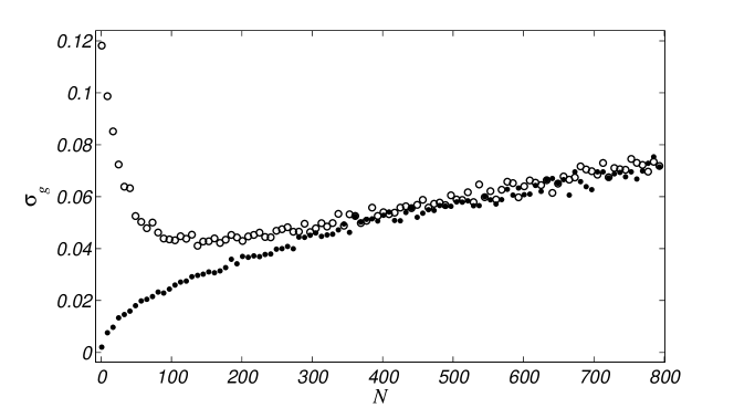
Figure 1: The plot shows the numerically estimated variance of the geometric phase angle for a particle in a monopole field. The variance is plotted as a function of the average number of noise fluctuation for a Ornstein-Uhlenbeck process modeling the noise component, with amplitude $\epsilon=0.05$. The data represented by dots refer to a trivial drift loop (purely Brownian motion), they are well fitted by a square root law $\sigma_{g}=a\sqrt{N}+b$, with $a\simeq 0.0025$ and $b=-0.00016$. The data represented by circles correspond to the drift loop in equation (13) (Brownian motion superimposed to precession).

5 Conclusion

We have computed the mean value and the variance of the Dirac phase acquired by a semiclassical particle subjected to Brownian motion. If the trajectory is purely Brownian the variance of the Dirac phase angle always increases as function of the operational time (or the average number of noise fluctuations). On the other hand, a transient behavior is observed if the Brownian motion is superimposed to a noiseless drift loop.

In the case of pure Brownian motion, we have obtained an expression for the variance which is of the second order in the amplitude of noise and increases with the operational time. In particular, if the noise is modeled by a Ornstein-Uhlenbeck process the variance grows with the square root of the operational time.

The case of the Dirac phase can be viewed as instance of geometric phase. Hence we can compare our results to others which refer to Berry phase. In [19], it was shown that in the case of an adiabatic precession of a $1/2$-spin the leading term in the variance of the Berry phase is of the first order in the amplitude of the noise. Moreover, this terms decrease linearly with the operational time. This behavior is in accordance with the transient behavior of the Dirac phase for nontrivial noiseless drift loop. Notice that the second order effects become relevant for long enough operational time.

At the best of our knowledge, the presentation of the effects of second order in the variance of the Dirac phase introduces a new element in the study of the robustness of geometric phases. We argue that second order effects are feasible to be observed in experimental settings as in [21]. Recently, the effects of non-adiabaticity in the noise component were studied in [24]. The pattern of the variance of the corresponding geometric phase as function of the operational time is qualitative analogous to the results presented here, in the sense that the squared variance grows linearly in time. Quantitatively, this effect is of the first order in the noise amplitude in [24] while in our analysis, which assumes the adiabatic approximation, the effect of the second order.

References

- [1] S. Pancharatnam, Proc. Indian Acad. Sci. A 44 247 (1956); reprinted in Collected works of S. Pancharatnam (Oxford Univ. Press, London, 1975)
- [2] M. V. Berry, Proc. R. Soc. Lond. A 392 45 (1984)
- [3] B. Simon, Phis. Rev. Lett. 51 2167 (1983)
- [4] F. Wilczek and A. Zee, Phis. Rev. Lett. 52 2111 (1984)
-
[5]
Y. Aharonov, J. Anandan,
Phis. Rev. Lett. 58 1593 (1987);
J. Anandan, Phys. Lett. A 133 171 (1988) - [6] J. Samuel and R. Bhandari, Phis. Rev. Lett. 60 2339 (1988)
- [7] A. Bohm, A. Mostafazadeh, H. Koizumi, Q. Niu and J. Zwanziger The Geometric Phase in Quantum Systems (Heidelberg: Springer-Verlag, 2003)
-
[8]
C. H. Bennett and G. Brassard,
Quantum Cryptography: Public Key Distribution and Coin
Tossing, Proceedings of IEEE International Conference on Computers
Systems and Signal Processing, Bangalore India (1984);
A. K. Ekert, Phis. Rev. Lett. 67 661 (1991);
P. W. Shor, SIAM J. Sci. Statist. Comput. 26 1484 (1997) - [9] M. A. Nielsen, I. L. Chuang, Quantum Computation and Quantum Information (Cambridge University Press, Cambridge, 2000)
- [10] P. Zanardi, M. Rasetti, Phys. Lett. A 264 94 (1999)
- [11] D. Deutsch, Proc. R. Soc. Lond. A 400 97 (1985)
- [12] G. Falci, R. Fazio, G. M. Palma, J. Siewert, and V. Vedral, Nature 407 355 (2000)
- [13] L. M. Duan, J. I. Cirac, P. Zoller, Science 292 1695 (2001)
- [14] D. Leibfried, B. De Marco, V. Meyer, D. Lucas, M. Barrett, J. Britton, W. M. Itano, B. Jelenkovic, C. Langer, T. Rosenband, and D. J. Wineland, Nature 422 412 (2003)
- [15] M. Tian, Z. W. Barber, J. A. Fischer, and W. Randall Babbitt, Phys. Rev. A 69 050301(R) (2004)
- [16] J. A. Jones, V. Vedral, A. Ekert and G. Castagnoli, Nature 403 869 (2000)
-
[17]
P. W. Shor,
Phys. Rev. A 52 2493 (1995);
A. Steane, Proc. R. Soc. Lond. A 452 2551 (1996);
A. R. Calderbank and P. W. Shor, Phys. Rev. A 54 1098 (1996) - [18] A. Y. Kitaev, Ann. Phys. 303 2 (2003)
- [19] G. De Chiara, G. M. Palma, Phys. Rev. Lett. 91 090404 (2003)
-
[20]
P. Solinas, P. Zanardi and N. Zanghì,
Phys. Rev. A 70 042316 (2004);
G. Florio, P. Facchi, R. Fazio, V. Giovannetti and S. Pascazio, Phys. Rev. A 73 022327 (2006);
C. Lupo, P. Aniello, M. Napolitano, G. Florio, Phs. Rev. A 76 012309 (2007) - [21] S. Filipp, J. Klepp, Y. Hasegawa, C. Plonka-Spehr, U. Schmidt, P. Geltenbort, H. Rauch, arXiv:0812.3757v1 (2008)
- [22] C. W. Gardiner, Handbook of Stochastic Methods (Springer, Berlin, 1983)
- [23] D. T. Gillespie, Phys. Rev. E 54 2084 (1996)
- [24] X. J. Hou, Phys. Rev. A 75 024103 (2007)