A continuous, piecewise affine surface map with
no measure of maximal entropy

Abstract.

It is known that piecewise affine surface homeomorphisms always have measures of maximal entropy. This is easily seen to fail in the discontinuous case. Here we describe a piecewise affine, globally continuous surface map with no measure of maximal entropy.

1. Introduction

1.1. Measures of Maximal Entropy

The complexity of the orbit structure of a dynamical system is reflected by its topological entropy. Entropy can also be defined at the level of invariant probability measures. These two levels are related by the variational principle, i.e., for any continuous self-map of a compact metric space:

$$h_{\operatorname{top}}(f)=\sup_{\mu}h(f,\mu).$$

This brings to the fore maximal entropy measures, i.e., those having ”full complexity” in the following sense:

$$h(f,\mu)=h_{\operatorname{top}}(f).$$

Such measures may fail to exist, e.g., for any $r<\infty$, there are $C^{r}$ smooth interval maps with non-zero topological entropy and no maximal entropy measures [2, 10]. However, building on Yomdin’s theory [11] of smooth mappings, Newhouse has shown the following

1.1 Theorem (Newhouse [8]).

If $f$ is $C^{\infty}$ self-map of a compact manifold, then $\mu\mapsto h(f,\mu)$ is upper semicontinuous as a function on the compact set of invariant probability measures endowed with the weak star topology. In particular, there exists a maximal entropy measure.

1.2. Piecewise Affine Transformations

This does not apply to the following simple class of transformations, even under the assumption of global continuity:

1.2 Definition.

A map $T:M\to M$ is said to be piecewise affine if

1. $M$ is admits an affine atlas (i.e., a set of charts whose change of coordinates are affine diffeomorphisms);

2. there exists a finite partition of $M$ whose elements $A$ satisfy: (i) $A$, resp. $TA$, are each contained in the domain of a chart $\chi$, resp. $\chi^{\prime}$, of the affine atlas; (ii) $\chi^{\prime}\circ T\circ\chi^{-1}|A$ is the restriction of an affine map to some open subset of some $\mathbb{R}^{d}$.

However, Newhouse observed [9, 4] that the above property nevertheless holds for piecewise affine surface homeomorphisms. This follows from the sub-exponential rate at which discontinuities can accumulate when one iterates the map: the multiplicity entropy introduced in [3] is zero for such maps.

Additionally, the set of maximal entropy measures of such transformations has been shown [4] to be a finite-dimensional simplex whenever $h_{\operatorname{top}}(f)\neq 0$.

It is easy to see that the finiteness property fails for piecewise affine continuous maps. Indeed, it is enough to consider the direct product of the identity on some interval with a piecewise affine, globally continuous interval map with nonzero entropy.

1.3. Main Result

In this note we show that existence also fails to hold generally for such maps:

1.3 Theorem.

There exists a piecewise affine, globally continuous map $T$ of $[0,1]^{2}$ satisfying $h_{\operatorname{top}}(T)=\sup_{\mu}h(T,\mu)=\log 2$ with no maximal entropy measure, i.e., no measure achieving this supremum.

This map will be explicitly described. Taking the direct product of the above map with the identity of a cube of the proper dimension, one immediately obtains the following:

1.4 Corollary.

For any integer $d\geq 2$, there exists a piecewise affine, globally continuous map $T$ of $[0,1]^{d}$ satisfying $h_{\operatorname{top}}(T)=\sup_{\mu}h(T,\mu)=\log 2$ with no maximal entropy measure, i.e., no measure achieving this supremum.

1.4. Comments

We can compare globally continuous, piecewise affine maps to related classes for which this problem has been studied.

On the one hand, existence is known to fail if one removes:

• either the continuity assumption. We refer to [3, 6, 7] for examples and more discussion, including failure of the variational principle.

• or the affine assumption. It is easy to construct a globally continuous, piecewise quadratic map without a measure of maximal entropy [4]. This construction is derived from examples of $C^{\infty}$ maps at which the topological entropy fails to be lower semi-continuous.

On the other hand, a classical theorem of Hofbauer [5] asserts that existence and finiteness hold for piecewise affine interval maps (in fact, piecewise monotone maps) with non zero entropy.

2. General Description of the Map

2.1. Key Properties

The map $T$ is defined on a parallelogram $Q:=ENWS$ (we write $X_{1}\dots X_{k}$ for the compact polygon with sides $[X_{1}X_{2}],\dots,[X_{k}X_{1}]$).

Define the vertical cone

$$\mathcal{C}^{s}:=\left\{\left(\begin{matrix}x\\ y\end{matrix}\right):|x|\leq 2|y|\right\}.$$

We say that $\mathcal{C}^{s}$ is stable for some map, if the differential at any point of the inverse of that map (where this differential exists) sends $\mathcal{C}^{s}$ into itself.

Let us describe the key properties of the map $T$ (see Fig. 1):

1. the poles $N$ and $S$ are fixed points;

2. all points in the top half $NWE$ (the grey triangle in Fig. 1) are attracted to $N$;

3. each one of the red triangles $ABS$ and $CDS$ is mapped to the large triangle $ADS$;

4. $T|ABS$ divides the $y$-coordinate by a factor $\leq 2$;

5. $T|CDS$ multiplies the $y$-coordinate by a factor of $2$;

6. $\mathcal{C}^{s}$ is stable for the map on $ABS\cup CDS$;

7. on $ABS\cup CDS$, the map preserves the horizontal and expands horizontal vectors by a factor $\geq 4$;

8. the middle, green-blue part $BCS$ is mapped into the blue, right side $DES$, except for a part which is mapped into $NEW$ after one or two iterations of $T$;

9. $DES$ is mapped into the purple left side $WAS$ and $NWE$;

10. all orbits starting in $WAS$ eventually converge to fixed points.

To be precise, we must state the following corrections, involving the exact partition defined below:

Properties (3)-(7) do not hold on the top parts $ABA^{t}B^{t}$ and $CDC^{c}D^{c}$ which are mapped into $NEW$. The contraction is exactly by a factor of $2$ on the lower part, $A^{c}B^{c}S$, of $ABS$.

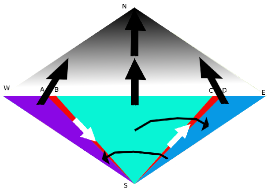
Figure 1. Main zones for the dynamics of the example $T$

2.2. Precise definition of the map

The above is realized as a piecewise affine, globally continuous map $T:Q\to Q$. The parallelogram $Q=NWES$ is partitioned into 26 triangles, on each of which the map is affine.

The $x$-coordinates of the vertices of this partition which lie on the diagonal $y=y^{1}$ are given in Table 1. The top and bottom points of $Q$ are $N(0,2)$ and $S(0,0)$. The other vertices of the partition are obtained from those on $y=y^{1}$ by homotheties centered at $S$ or $N$ yielding points on $y=y^{u},y^{t},y^{c},y^{b}$ with values in Table 2. We denote by $A^{t}$ the vertex obtained from $A$ on the line $y=y^{t}$, etc. The resulting partition and vertices are depicted in Fig. 2.

Name	W	A	B	O	C	D	E
$x$	-1.5	-1	-0.9	0	0.9	1	1.5

Table 1. $x$-coordinates of the vertices on the line $y=y^{1}$.

Name	$y^{1}$	$y^{t}$	$y^{c}$	$y^{b}$	$y^{u}$
$y$	1	0.8	0.5	0.25	1.5

Table 2. $y$-coordinates of the horizontal lines used to define $T$.

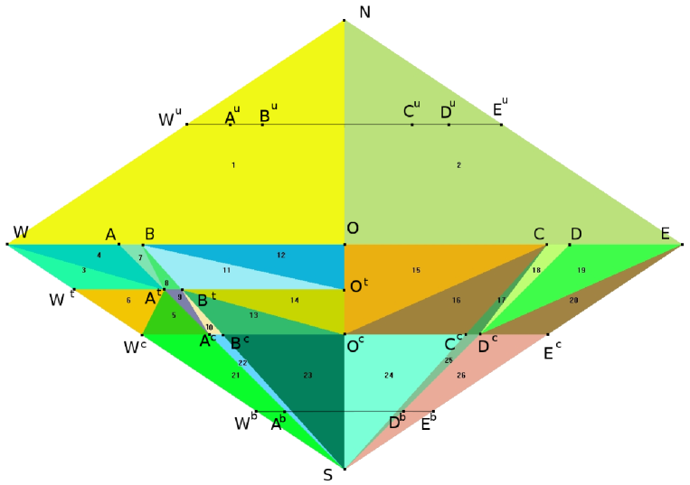
Figure 2. Partition and special points for the map $T$.

The piecewise affine map is finally defined by the images of the vertices of the partition, as given in Table 3.

On $y=y^{1}$	$W$	$A$	$B$	$O$	$C$	$D$	$E$
Image	$W^{u}$	$A^{u}$	$D^{u}$	$E^{u}$	$D^{u}$	$A^{u}$	$W^{u}$
On $y=y^{t}$	$W^{t}$	$A^{t}$	$B^{t}$	$O^{t}$	—	—	—
Image	$W$	$A$	$D$	$E$	—	—	—
On $y=y^{c}$	$W^{c}$	$A^{c}$	$B^{c}$	$O^{c}$	$C^{c}$	$D^{c}$	$E^{c}$
Image	$W^{c}$	$A^{b}$	$D^{b}$	$E^{c}$	$D$	$A$	$W$

Table 3. Mapping of the points. Note: the remaining vertices, $S$ and $N$, are fixed points.

2.3. Proof of the Key Properties

Key properties (1) and (2) are immediate from $T(S)=S$, $T(N)=N$ and the fact that $T|NWO$ and $T|NEO$ are affine map with $W,O,E$ mapped strictly above the line $(WE)$.

A direct computation shows that the preimage of $NWE$ is the union of $NWE$ with $WW^{t}OO^{t}$, $C^{c}E^{c}CE$ and some upper part of $OO^{c}CC^{c}$ —see Fig. 3. Using this, the following shows the key properties (3)-(7).

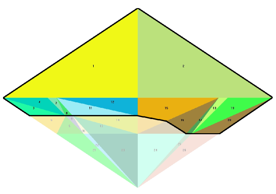
Figure 3. $T^{-1}(NEW)$ delineated by a bold line.

Key property (3) follows by inspection, see Fig. 4. Looking at Table 4 we see that $T^{\prime}|A^{t}B^{t}S$ multiplies the $y$-coordinate by $0.5$ or $2.5$, proving (4), $0.5$ on $A^{c}B^{c}S$. (5) is checked in the same way.

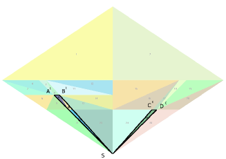
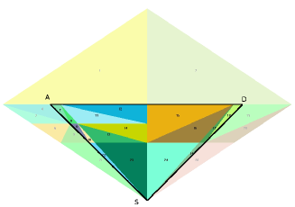
Figure 4. On the left: the triangles $A^{t}B^{t}S$ and $C^{c}D^{c}S$. On the right: their (identical) image. The bold lines on the right are the images of those on the left.

We are going to prove that $\mathcal{C}^{s}$ is stable for $T|A^{t}B^{t}S$ and $T|C^{c}D^{c}S$. We have to check this property for the $4$ affine maps involved using the following:

2.1 Lemma.

Let $A=\left(\begin{matrix}a&b\\ c&d\end{matrix}\right)$. The following is a sufficient condition for the invariance $A^{-1}(K_{C})\subset K_{C}$ where $K_{C}:=\{\left(\begin{matrix}x\\ y\end{matrix}\right):|x|\leq C|y|\}$:

$$\gamma_{1}:=C|c/a|<1\text{ and }\gamma_{2}:=\frac{|d|+|b|C^{-1}}{|a|-C|c|}\leq 1.$$

Proof.

Let $\left(\begin{matrix}\xi^{\prime}\\ \eta^{\prime}\end{matrix}\right)=A\left(\begin{matrix}\xi\\ \eta\end{matrix}\right)$ with $|\xi^{\prime}|\leq C|\eta^{\prime}|$. We have

$$\xi=a^{-1}\xi^{\prime}-a^{-1}b\eta\text{ and }\eta^{\prime}=c\xi+d\eta.$$

Hence, abreviating $|a|,|b|,\dots$ to $a,b,\dots$,

$$|\xi|\leq a^{-1}|\xi^{\prime}|+a^{-1}b|\eta|\leq Ca^{-1}(c|\xi|+d|\eta|)+a^{-1}b|\eta|.$$

Thus,

$$(1-a^{-1}cC)|\xi|\leq(a^{-1}dC+a^{-1}b)|\eta|.$$

If the first factor is positive this is equivalent to

$$|\xi|\leq\frac{a^{-1}dC+a^{-1}b}{1-a^{-1}cC}.$$

The Lemma follows. ∎

Triangle	$A^{c}B^{c}S$	$A^{t}B^{t}A^{c}$	$A^{c}B^{t}B^{c}$	$C^{c}D^{c}S$
Matrix	$10\quad 9.5$	$25\quad 22.5$	$10\quad 11.5$	$-40\quad 38$
	$\;0\quad 0.5$	$\;0\quad 2.5$	$\;0\quad 2.5$	$0\quad 2$
$\gamma_{1}$	$0$	$0$	$0$	$0$
$\gamma_{2}$	$0.525$	$0.55$	$0.825$	$0.525$

Table 4. Stability of the cone.

The matrices of the linear parts of the $4$ affine maps are listed in Table 4 together with the quantities denoted above $\gamma_{1},\gamma_{2}$ for each of those. Thus (6) holds.

Property (7) also follows immediately from the matrices in Table 4 (the left lower entry is zero and the left upper entry is bigger than $4$ in absolute value).

To prove that the ”folding zone” $BCS$ is mapped to the right of $CDS$ except for the part that ends up in $NEW$ in one or two iterations, we decompose it into its left half $BOS$ and right half $OSC$ —see Fig. 5. The images are given in Fig. 6. We see that $T(BOS)\subset DES\cup NEW$ and the image of $T(OSC)\subset DES\cup NEW\cup\Delta$ where $\Delta\subset OO^{c}CC^{c}$ is itself mapped into $NEW$ according to Fig. 3. This proves property (8).

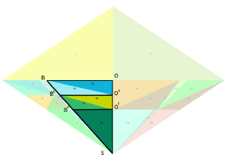
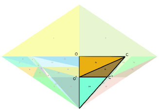
Figure 5. The two halves of the folding zone: $BOS$ on the left and $OSC$ on the right.

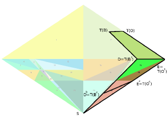
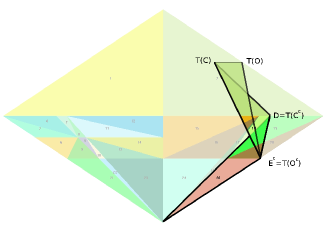
Figure 6. The images of two halves of the folding zone: $T(BOS)$ on the left and $T(OSC)$ on the right. The bold lines are the images of those in Fig. 5.

Similarly one checks that $DES$ and $WAS$ (see Fig. 7) are both mapped to subsets of $WAS\cup NEW$ (see Fig. 8). This establishes property (9) and prepares the proof of (10).

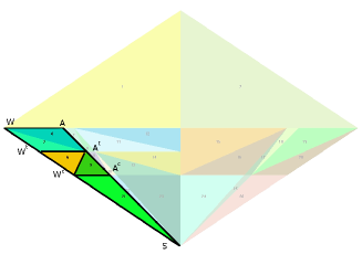
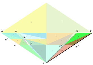
Figure 7. The two triangles $(WAS)$ on the left and $(DES)$ on the right.

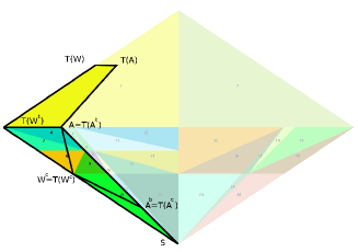
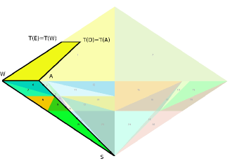
Figure 8. The images of $(WAS)$ on the left and $(DES))$ on the right. The bold lines are the image of those in Fig. 7.

2.4. Orbits not contained in $A^{t}B^{t}S\cup C^{c}D^{c}S$

By the above remarks, such orbits must eventually land in $NEW$ –in which case they converge to the fixed point $N$; or enter $WAS$ and stay there for ever.

Let us show that an orbit which is confined to $WAS$ converges to a fixed point. $WAS$ is the union of $5$ triangles on each of which the map is affine: the triangles numbered $3,4,5,6$ and $21$ on Fig. 2.

As pictured in Fig. 3, the triangles $3$ and $4$ are mapped into $NEW$ so our orbit cannot enter them. As can be seen in Fig. 8, the triangle $21$ (i.e., $W^{c}A^{c}S$) is mapped into itself. Moreover the segment $[W^{c}S]$ is made of fixed points, while the transverse direction is contracted like $[A^{c}S]$. It follows that all points in this triangle eventually converge to some fixed point in $[W^{c}S]$.

Triangle $6$, i.e., $W^{t}W^{c}A^{t}$, is mapped to $WW^{c}A$ which is contained in $W^{t}W^{c}A^{t}\cup T^{-1}NEW$. But

$$T^{\prime}(x,y)=\left(\begin{matrix}\frac{5}{4}&\frac{5}{8}\\ 0&\frac{5}{3}\end{matrix}\right)$$

with eigenvalues are $5/3$ and $5/4$: it is expanding. Thus all points in triangle 6, except the fixed point $W^{c}$ are eventually mapped into $NEW$ under positive iteration.

We consider triangle $5$, i.e., $W^{c}A^{c}A^{t}$. Using Fig. 8, observe that points that exit this triangle cannot re-enter it. Hence it is enough to analyze orbits that stay in $W^{c}A^{c}A^{t}$ forever. However, on that triangle,

$$T^{\prime}(x,y)=\left(\begin{matrix}2&-\frac{1}{2}\\ -1&\frac{3}{2}\end{matrix}\right)$$

with eigenvalues: $2.5$ and $1$, the latter with eigenvector $\left(\begin{matrix}1\\ 2\end{matrix}\right)$. As $T(W^{c})=W^{c}$, this gives a segment of fixed points for the affine map and everything else is eventually mapped outside of the triangle.

This completes the proof of property (10) and therefore of all the key properties.

3. Proof of the Theorem

In this section, we deduce the Main Theorem from the key properties (1)-(10).

First, let us note that the only aperiodic ergodic, invariant measures are carried by the compact invariant set

$$K:=\bigcap_{n\geq 0}T^{-n}(ABS\cup CDS).$$

Indeed, by key properties (2), (8), (9) and (9) and the additional remark below them, all orbits which do not stay in $ABS\cup CDS$ for ever converge to fixed points.

We set $K_{0}:=K\setminus\{S\}$ and denote the $2$-shift by $\sigma:\Sigma\to\Sigma$ with $\Sigma:=\{0,1\}^{\mathbb{N}}$. The key fact is:

3.1 Lemma.

$(T,K_{0})$ is an entropy-preserving extension of a subset of the $2$-shift according to

$$\gamma:x\in K_{0}\longmapsto(\epsilon_{n})_{n\geq 0}\in\Sigma\text{ where }\epsilon_{n}=0\iff T^{n}(x)\in ABS.$$

More precisely, $h(T,\mu)=h(\sigma,\gamma_{*}\mu)$ for any invariant probability measure $\mu$ of $(T,K_{0})$.

Proof.

$\gamma$ is clearly continuous and satisfies $\gamma\circ T=\sigma\circ\gamma$ on $K_{0}$. We claim that $\gamma^{-1}\gamma(x)$ is a $C^{1}$ curve starting from $S$, containing $x$ and whose tangent is everywhere contained in $C^{s}$ (we call such curves vertical).

Indeed, define, for any $n\geq 0$, $C_{n}(x):=\{y\in Q:\forall 0\leq k\leq n\;f^{n}y\in\gamma_{k}(x)\}$ where $\gamma_{k}(x)\in\{ABS,CDS\}$ is characterized by $T^{k}(x)\in\gamma_{k}(x)$. Note that $T(ABS),T(CDS)\supset ABS\cup CDS$. Hence $T^{n}C_{n}(x)=ABS$ or $CDS$.

According to (4)-(5), $\mathcal{C}^{s}$ is stable by $T|ABS$ and $T|CDS$ and contains the vertical boundary lines of these two triangle (with equations $x=\kappa y$ with $|\kappa|\in\{0.9,1\}$, see Table 3). Thus $C_{n}(x)$ is bounded by two vertical curves and some graph $y=\phi(x)$. Moreover $(T^{n}|C_{n}(x))^{-1}$ is strongly contracting horizontally by (7). Therefore $\bigcap_{n\geq 0}C_{n}(x)$ is a vertical curve containing $x$.

To conclude, observe that this vertical curve is $\gamma^{-1}\gamma(x)$ and that the restriction of $T^{n}$ to this set for any $n\geq 0$ is a homeomorphism. Hence $h_{\operatorname{top}}(T,\gamma^{-1}\gamma(x))=0$. It follows from a result of Bowen [1] that $\gamma$ preserves the entropy (the requirement of compactness can be fulfilled by replacing $K_{0}$ with its image under $(x,y)\mapsto(x/y,y)$, compactified by the addition of $\Sigma$). ∎

3.2 Lemma.

$T$ satisfies: $h_{\operatorname{top}}(T)=\log 2$.

Proof.

As a continuous map, $T$ satisfies: $h_{\operatorname{top}}(T)=\sup_{\mu}h(T,\mu)$. The above lemma shows that one can restrict this supremum to invariant measures carried by $K_{0}$ and that these measures have entropy at most $\log 2$, proving $h_{\operatorname{top}}(T)\leq\log 2$. For the reverse implication, we use that $T|A^{c}B^{c}S$ and $T|C^{c}D^{c}S$ are linear, multiplying the $y$-coordinate by $1/2$ and $2$ respectively. It follows that if $(x_{k},y_{k}):=T^{k}(x_{0},y_{0})$ belongs to these two small triangles near $S$ for $0\leq k<n$, then:

$$\log y_{n}=\log y_{0}+\log 2\cdot\sum_{k=0}^{n-1}\operatorname{sign}(x_{k}).$$

Let $M$ be a large integer. Let

$$\Sigma_{M}:=\biggl{\{}\alpha\in\Sigma:\forall p<q\;\bigl{|}\sum_{k=p}^{q}(\alpha_{k}-\frac{1}{2})\bigr{|}\leq M\biggr{\}}.$$

It is clearly compact and invariant, i.e., a subshift. We claim that: $\lim_{M\to\infty}h_{\operatorname{top}}(\Sigma_{M})=\log 2$.

Indeed, let $B(N):=\{A\in\{0,1\}^{2N}:\sum_{k=0}^{2N-1}A_{k}=N\}$ and

$$\Sigma^{\prime}_{M}:=\bigcup_{k=0}^{2N-1}\{A^{1}A^{2}\dots:A^{n}\in B(N)\}$$

This is a subshift of $\Sigma_{2N}$ with entropy $\log\#B(N)/2N$ which converges to $\log 2$. The claim is proven.

Let

$$X_{M}:=\{(\alpha,s)\in\Sigma_{M}\times\{-M,\dots,M\}:\forall p\in{\mathbb{N}}\;\bigl{|}\frac{s}{2}+\sum_{k=0}^{p}(\alpha_{k}-1/2)\bigr{|}\leq\frac{M}{2}\}$$

and define $F_{M}:X_{M}\to X_{M}$ by $F_{M}(\alpha,s)=(\sigma(\alpha),s+(\alpha_{0}-1/2))$. It is easy to check that this is a well-defined, finite, topological extension of $\Sigma_{M}$. Also it can be embedded into $K_{0}\cap\{2^{-M}y^{c}\leq y\leq y^{c}\}$ by the map $\iota_{M}$ defined by:

$$\iota_{M}(\alpha,s)=(y(s)x(\alpha),y(s))$$

where

$$x(\alpha):=-\frac{19}{20}\sum_{n\geq 0}\frac{\sigma_{0}\dots\sigma_{n}}{20^{n}}\text{ and }y(s):=y^{c}2^{s-M/2}$$

Embedding a measure maximizing entropy of $F_{M}$ into $T$ through $\iota_{M}$ and letting $M\to\infty$ shows that $h_{\operatorname{top}}(T)=\log 2$. ∎

3.3 Proposition.

$T$ has no invariant probability measure with entropy $\log 2$.

Proof.

We proceed by contradiction, assuming the existence of such a measure, say $\mu$. By the previous lemma, it is supported by $K_{0}$. Hence $\gamma_{*}\mu$ is an invariant probability measure of the full shift with entropy $\log 2$. It must be the $(\frac{1}{2},\frac{1}{2})$-Bernoulli measure. Thus, noting as above $(x_{k},y_{k}):=T^{k}(x_{0},y_{0})$, we have:

$$\mu-\forall(x_{0},y_{0})\qquad\sup_{n\geq 0}\sum_{k=0}^{n}\operatorname{sign}(x_{k})=\infty.$$

Now,

$$\log y_{n}=\log y_{0}+\sum_{k=0}^{n-1}\log\frac{y_{k+1}}{y_{k}}$$

and $y_{k+1}\geq 2^{\operatorname{sign}(x_{k})}y_{k}$ by key properties (4)-(5). Hence, $\sup_{n\geq 0}y_{n}=\infty$, a contradiction. ∎