Two-slit diffraction with highly charged particles: Niels Bohr’s consistency argument that the electromagnetic field must be quantized

Abstract

We analyze Niels Bohr’s proposed two-slit interference experiment with highly charged particles that argues that the consistency of elementary quantum mechanics requires that the electromagnetic field must be quantized. In the experiment a particle’s path through the slits is determined by measuring the Coulomb field that it produces at large distances; under these conditions the interference pattern must be suppressed. The key is that as the particle’s trajectory is bent in diffraction by the slits it must radiate and the radiation must carry away phase information. Thus the radiation field must be a quantized dynamical degree of freedom. On the other hand, if one similarly tries to determine the path of a massive particle through an inferometer by measuring the Newtonian gravitational potential the particle produces, the interference pattern would have to be finer than the Planck length and thus undiscernable. Unlike for the electromagnetic field, Bohr’s argument does not imply that the gravitational field must be quantized.

Niels Bohr once suggested a very simple gedanken experiment to prove that, in order to preserve the consistency of elementary quantum mechanics, the radiation field must be quantized as photons footnote1 . In the experiment one carries out conventional two-slit diffraction with electrons (or other charged particles), building up the diffraction pattern one electron at a time (as in the experiment of Ref. tonomura ). One then tries to determine which slit the electron went through by measuring far away, in the plane of the slits, the Coulomb field of the electron as it passes through the slits. See Fig. 1. If the electron passes through the upper slit it produces a stronger field than if it passes through lower slit. Thus if one can measure the field sufficiently accurately one gains “which-path” information, posing the possibility of seeing interference while at the same time knowing the path the electron takes, a fundamental violation of the principles of quantum mechanics footnote2 .

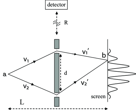
Figure 1: Two slit diffraction with single electrons, in which one measures the Coulomb field produced by the electrons at the far-away detector.

In an experiment with ordinary electrons of charge $e$ the uncertainty principle prevents measurement of the Coulomb field to the required accuracy, as we shall see below, following the prescription of Bohr and Rosenfeld for measuring electromagnetic fields BR1933 ; BR1950 . However, as Bohr pointed out, one can imagine carrying out the same experiment with (super) electrons of arbitrarily large charge, $Ze$, and indeed, for sufficiently large $Z$, one can determine which slit each electron went through. However, elementary quantum mechanics requires that once one has the capability of obtaining which-path information, even in principle, the interference pattern must be suppressed, independent of whether one actually performs the measurement.

Underlying the loss of the pattern is that the electron not only carries a Coulomb field, but also produces a radiation field as it ”turns the corner” when passing through the slits. The larger the charge the stronger is the radiation produced. This radiation must introduce a phase uncertainty in order to destroy the pattern, and so itself must carry phase information; thus the electromagnetic field must have independent quantum degrees of freedom. Were the quantum mechanical electrons to emit classical radiation, the emission would produce a well-defined phase shift of the electron amplitudes along the path, which while possibly shifting the pattern, as in the Aharonov-Bohm effect aharonov-bohm , would not destroy it. In a sense the suppression of the pattern is an extension of the Aharonov-Bohm effect to fluctuating electromagnetic potentials (discussed by Aharonov and Popescu footnote3 ).

Our object in this paper is to carry out a detailed analysis of the physics implicit in Bohr’s suggested experiment. After describing the experiment more fully, we determine the strength of charge needed to measure the Coulomb field at large distances sufficiently accurately. We then analyze how coupling of the particle to the quantized electromagnetic field in diffraction suppresses the interference pattern, with increasing charge, before Coulomb measurements can yield which-path information.

The first experiment that revealed effects of quantization of the electromagnetic field in interference is that of Grangier et al. aspect , which showed how interference of single photons differs from classical interference. The loss of particle coherence in interferometry due to photon emission was first demonstrated by Pfau et al. pfau , and due to photon scattering by Chapman et al chapman . Various works, both theoretical and experimental, have discussed determining the path of charged particles in the double-slit problem, but none, it seems, in connection with Bohr’s proposed experiment. The theoretical possibility of distinguishing paths by measurement of the photon field is discussed in Ref. scully , while Refs. furry and popescurmp discuss determining the path through detection of the electric field inside the loop of the paths. See also Stern et al. stern on decoherence due to the interaction of charged particles with the gauge field. Experimental attempts to measure which-path information using interferometers fabricated in high-mobility two-dimensional electron gases include Refs. schuster ; buks ; chang .

A natural question to ask is whether by measuring the Newtonian gravitational field produced by the mass of a particle as it diffracts, one can similarly gain which-path information; as we show, the answer is that one can, for sufficiently large mass. However, one cannot conclude in this case that the gravitational field must also be quantized, since for masses for which one can determine the path, the fringe separation in the diffraction pattern would shrink to below the Planck length, $\ell_{\rm pl}=(G\hbar/c^{3})^{1/2}$, where $G$ is Newton’s gravitational constant and $c$ is the speed of light. However, position measurements are fundamentally limited in accuracy to scales $\mathrel{\hbox to0.0pt{\raise 2.20013pt\hbox{$>$}\hss}{\lower 2.20013pt\hbox{$\sim$}}}\ell_{\rm pl}$ calmet , and thus distinguishing so a fine pattern cannot be carried out. Unlike in the electromagnetic case, where the interference pattern is suppressed due to decoherence caused by the radiated photons, the pattern in the gravitational case becomes immeasurably fine, not because the particles radiate quantized gravitons.

I Measurement of the Coulomb field

In the experiment sketched in Fig. 1 a charged particle enters the apparatus from the left side, goes through a double slit, and hits the screen ($b$). The spacing of the slits is $d$, and $L$ is the distance from the particle emitter ($a$) to the screen. The Coulomb field of the electron is measured at distance $\sim R$ in the plane of the slits, sufficiently far away from the apparatus that there can be no back-reaction from the distant measurement of the electromagnetic field. Thus $R\mathrel{\hbox to0.0pt{\raise 2.20013pt\hbox{$>$}\hss}{\lower 2.20013pt\hbox{$\sim$}}}cT$, where $T$ is the time of the flight of the particle, $\simeq L/v$, with $v$ the particle velocity. We consider only non-relativistic particles, in which case the longitudinal Coulomb field of the electron at distance $R\sim cT$ is larger than the transverse radiation field by a factor $\sim c/v$. We assume that the Coulomb field is determined by the charge in the usual manner.

To distinguish whether the particle goes through the upper or lower slit one needs to measure the electric field to at least an accuracy $Ze(1/R^{2}-1/(R+d)^{2})\sim Zed/R^{3}$ (with $d\ll R$). The quantum limit on the measurability of a weak electric field $E$ was obtained by Bohr and Rosenfeld BR1933 ; BR1950 . In an early discussion of such a quantum measurement, Landau and Peierls LP1931 noted that if one attempts to measure the field by its effect on a point charge, radiation recoil introduces uncertainties in the measurement that diverge for short measuring times, and thus concluded that “in the quantum range …the field strengths are not measurable quantities.” To avoid this problem, Bohr and Rosenfeld envisioned measuring the average of the electric field over a region of space-time, using an extended apparatus consisting of an object $A$ of mass $M$ and volume $V_{A}$ with extended charge $Q$, tethered by Coulomb forces to a similar object $B$ with background charge $-Q$. See Fig. 2. The background charge is fixed in space, but $A$ is displaced by an electric field from its equilibrium position. The apparatus measures the field by detecting the deflection of $A$ from its equilibrium position. The net equilibrium charge density of the apparatus is zero in the absence of an external field that displaces the object from the background. In their analysis they first assume quantization of the electromagnetic field, and show how vacuum fluctuations of the field in the region limit the accuracy of field measurements. They then go on to show that the accuracy of the measurement of a single field is limited by the uncertainty principle applied to the apparatus, without the need to invoke field quantization. We give a schematic derivation of this result (see also the recent discussions in Refs. compagno ; hnizdo ; saavedra .)

The relative motion of $A$ and $B$ is a harmonic oscillator whose frequency $\omega$ is readily derived from the familiar expression for the plasma frequency ($\omega_{p}^{2}=4\pi ne^{2}/m$), namely $\omega^{2}=4\pi Q^{2}/MV_{A}$. When $A$ is displaced relative to $B$ by a distance $x$, the restoring force acting between them is

$$F=-M\omega^{2}x=-4\pi Q^{2}x/V_{A}.$$ (1)

Thus, an external field $E_{x}$ acting on $A$ for time $T^{\prime}$ changes the momentum of $A$ by $p_{x}=(E_{x}Q-4\pi Q^{2}x/V_{A})T^{\prime}$, from which one would deduce an electric field,

$$E_{x}=4\pi Qx/V_{A}+p_{x}/QT^{\prime}.$$ (2)

Since $p_{x}$ and $x$ obey the uncertainty relation, $\delta x\delta p_{x}\mathrel{\hbox to0.0pt{\raise 2.20013pt\hbox{$>$}\hss}{\lower 2.20013pt\hbox{$\sim$}}}\hbar$, we see from minimizing the right side of Eq. (2) with respect to $\delta x$ that the uncertainty in the measurement of $E_{x}$ is independent of $Q$, and given by the Bohr-Rosenfeld relation, $\delta E_{x}\sim\sqrt{\hbar/V_{A}T^{\prime}}$. For simplicity we assume cubic geometry of $A$ and $B$, with $V_{A}=\xi^{3}$, The measurement time $T^{\prime}$ is at most the time of flight, $T$, since further increasing the measurement time does not help to distinguish the paths; thus we take $T^{\prime}=T$. In addition the length $\xi$ of interest is at most the Coulomb pulse width, $cT$, since a longer size does not help to distinguish the paths either. With $\xi=cT$, we obtain the limit of accuracy of the measurement of the Coulomb field:

$$\delta E_{x}\sim\sqrt{\frac{\hbar}{\xi^{3}T}}\,\,.$$ (3)

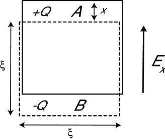
Figure 2: Bohr-Rosenfeld apparatus for measuring the electric field. The positively charged object $A$ slides on the negatively charged fixed object $B$.

To estimate the critical scale of charge of particles above which one begins to be able to distinguish the path, we take the measuring apparatus to be located from $R$ to $R+\xi$ above the upper slit. Then, when a particle with charge $Ze$ passes through the upper slit, the average Coulomb field in the apparatus is

$$\frac{1}{\xi}\int_{0}^{\xi}\frac{Ze}{(R+x)^{2}}dx=\frac{Ze}{R(R+\xi)}.$$ (4)

Similarly, the average electric field when the particle passes through the lower slit is $Ze/(R+d)(R+d+\xi)$, where $d$ is the slit interval. Hence to distinguish the paths the apparatus needs to distinguish an electric field difference

$$\Delta E=\frac{Ze(2R+\xi)}{R^{2}(R+\xi)^{2}}d,$$ (5)

a decreasing function of $\xi$. Since to measure the path, one needs $\Delta E>\delta E$ (the measurement uncertainty), or

$$Ze\mathrel{\hbox to0.0pt{\raise 2.20013pt\hbox{$>$}\hss}{\lower 2.20013pt\hbox{$\sim$}}}\frac{R^{2}(R+\xi)^{2}}{d(2R+d)}\sqrt{\frac{\hbar}{\xi^{3}T}}.$$ (6)

With $\xi\sim R\sim cT$ we find that the scale of critical charge $Z_{1}$ above which one can begin to distinguish the path is

$$Z_{1}\simeq\frac{1}{\sqrt{\alpha}}\frac{cT}{d},$$ (7)

where $\alpha=e^{2}/\hbar c$ is the fine structure constant. Note that $Z_{1}\gg 1$, so that one could never detect the path with ordinary electrons or other particles of charge $\sim|e|$. For illustration, from the parameters corresponding to the experiment of Ref. tonomura : $d\sim 1$ $\mu$m, and $cT\approx 6$ cm, we estimate $Z_{1}\simeq 7\times 10^{5}$.

One can in fact, for general $Z$, determine partial information on the paths, the amount of information increasing with $Z$. Writing $p(D_{u},l)$ as the probability of the particle having taken the lower path and the detector detecting it to have taken the upper path, $p(D_{u},u)$ as the probability of the particle having taken the upper path and the detector detecting it to have taken the upper path, etc., one can quantify the information in terms of the distinguishability $\mathcal{D}$ wooterszurek ; jaeger ; englert ; jacques

$$\mathcal{D} =\left|p(D_{u},u)-p(D_{l},u)\right|+\left|p(D_{l},l)-p(D_{u},l)\right|.$$ (8)

Since $p(D_{u},u)+p(D_{l},u)+p(D_{l},l)+p(D_{u},l)=1$, $\mathcal{D}\leq 1$.

To calculate $\mathcal{D}$ we note that the detector determines the electric field through simultaneous measurement of the position and momentum, which leads to a Gaussian uncertainty of width $\delta E$ in the measured value of the electric field from the expected value. For the particle taking the upper path, producing an expected (averaged) electric field $E_{u}$ at the detector, the probability distribution of the measured electric field is

$$P_{u}(E)=\frac{1}{\sqrt{2\pi}\delta E}e^{-(E-E_{u})^{2}/2\delta E^{2}},$$ (9)

with a similar expression for the field distribution $P_{l}(E)$ for the lower path in terms of the expected $E_{l}$. Since $E_{u}>E_{l}$, we can for simplicity regard the detector as having detected the particle taking the upper path if the measured value of the electric field is greater than $(E_{u}+E_{l})/2$, and as having taken the lower path otherwise.

With the assumption that the amplitudes for the particle taking the upper and the lower paths are equal in magnitude, which is true if the two slits are located symmetrically, then

$$p(D_{u},u)=\frac{1}{2}\int_{(E_{u}+E_{l})/2}^{\infty}P_{u}(E)dE=\frac{1}{2}-p(D_{l},u),$$ (10)

with similar equations for $p(D_{l},l)$ and $p(D_{u},l)$. With $\Delta E=E_{u}-E_{l}$, the distinguishability becomes

$$\mathcal{D}=\frac{1}{\sqrt{\pi}}\int_{-\Delta E/2\sqrt{2}\delta E}^{\Delta E/2\sqrt{2}\delta E}e^{-x^{2}}dx=\mathrm{erf}(Z/2\sqrt{2}Z_{1}),$$ (11)

where $\mathrm{erf}(x)$ is the error function. We plot $\mathcal{D}$ in Fig. 3 below for the parameters of Ref. tonomura .

II Loss of interference

We turn now to the question of how for sufficiently large charge (which should be $\mathrel{\hbox to0.0pt{\raise 2.20013pt\hbox{$<$}\hss}{\lower 2.20013pt\hbox{$\sim$}}}Z_{1}$) the interference pattern fades out. The basic physics is that the particle radiates when being accelerated by the slits, and undergoes a random change in its phase because it is coupled to a dynamical degree of freedom, the quantized radiation field. We do not take into account any quantum degrees of freedom associated with the slits, i.e., we assume that they act effectively as a potential on the electron. The pattern on the screen is proportional to $\sum_{f}\left(|\beta_{u}(b,f)+\beta_{l}(b,f)|^{2}\right)$ where $\beta_{u}(b,f)$ is the amplitude for the particle to go through the upper slit to point $b$ on the screen, with the electromagnetic field going from its initial state $|0\rangle$ (the vacuum) to final multi-photon state $|f\rangle$, and $\beta_{l}(b,f)$ is the amplitude for the particle to take the lower trajectory.

The interference pattern thus has the relative intensity,

$$I(b)=\frac{2{\rm Re}\sum_{f}\left(\beta_{l}(b,f)^{*}\beta_{u}(b,f)\right)}{\sum_{f}\left(|\beta_{u}(b,f)|^{2}+|\beta_{l}(b,f)|^{2}\right)}.$$ (12)

Although it is possible to carry out a full quantum calculation of the radiation emitted in diffraction, its essential features are brought out if we make the simplifying assumption that the charged particle follows a single straight trajectory along either the upper or lower path from the emission point $a$ to a given point $b$ on the screen (see Fig. 1). and thus the emitted radiation has only the effect of changing the phase of the electron amplitude. Then

$$\beta_{u}(b,f)\simeq\langle f|U_{u}|0\rangle\beta_{u}^{0},$$ (13)

where $\beta_{u}^{0}$ is the simple quantum amplitude in the absence of the electromagnetic field, and

$$U_{u}=\left(e^{(iZe/\hbar c)\int d{\vec{\ell}}\cdot\vec{A}(\vec{r},t)}\right)_{+},$$ (14)

where $\vec{A}(\vec{r},t)$ is the electromagnetic field operator, and the integral is time ordered (denoted by the subscript “+”) along the path. From Eq. (13),

$$\sum_{f}|\beta_{u}(b,f)|^{2}=\langle U_{u}^{\dagger}U_{u}\rangle|\beta_{u}^{0}|^{2}=|\beta_{u}^{0}|^{2},$$

$$\sum_{f}|\beta_{l}(b,f)|^{2}=|\beta_{l}^{0}|^{2},$$ (15)

and

$$\sum_{f}\beta_{l}(b,f)^{*}\beta_{u}(b,f)=\langle U_{l}^{\dagger}U_{u}\rangle{\beta^{0}_{l}(b)}^{*}\beta^{0}_{u}(b),$$ (16)

where the brackets denote the electromagnetic vacuum expectation value. Thus

$$\langle U_{l}^{\dagger}U_{u}\rangle=\big{\langle}\left(e^{(iZe/\hbar c)\int d{\vec{\ell}}\cdot\vec{A}(\vec{r},t)}\right)_{c}\big{\rangle},$$ (17)

where the subscript $c$ denotes the time ordering of the contour integral from emission to the screen along the upper path and then negatively time-ordered from the screen back to the emission point along the lower path. This expression is the expectation value of the Wilson loop around the path $u-l$ wilson . Since the free quantum electromagnetic field is Gaussianly distributed in the vacuum,

$$\langle U_{l}^{\dagger}U_{u}\rangle=e^{-(Z^{2}\alpha/2\hbar c)\Phi_{u-l}},$$ (18)

where

$$\Phi_{u-l}=\big{\langle}\left(\oint_{u-l}d\vec{\ell}\cdot\vec{A}(\vec{r},t)\right)_{c}^{2}\big{\rangle}.$$ (19)

Writing

$$\langle U_{l}^{\dagger}U_{u}\rangle={\cal V}e^{-i\zeta},$$ (20)

where the visibility ${\cal V}=|\langle U_{l}^{\dagger}U_{u}\rangle|$ is $\leq 1$, and the phase shift $\zeta$ is real, we have

$$I(b)=\frac{2{\rm Re}\left(\beta^{0}_{l}(b)^{*}\beta^{0}_{u}(b)e^{-i\zeta}\right)}{\left(|\beta^{0}_{u}(b)|^{2}+|\beta^{0}_{l}(b)|^{2}\right)}{\cal V}.$$ (21)

The coupling to the radiation field reduces the intensity of the interference pattern by ${\cal V}$, as well shifting it via $\zeta$. By symmetry, the shift vanishes at the center point on the screen (and is otherwise not relevant to the present discussion). Since the Coulomb field does not enter the states of the radiation field in ${\cal V}$, Eq. (21) gives a valid description of the interference pattern whether or not an attempt is made to distinguish paths by detecting the Coulomb field at large distances.

The real part of $\Phi_{u-l}$, entering the visibility, is given by the same integrals as in Eq. (19) without time ordering along the contour, since $\vec{j}(\vec{r},t)\cdot\vec{A}(\vec{r},t)$ is Hermitian ford1 :

$${\rm Re}\,\Phi_{u-l}=\big{\langle}\left(\oint_{u-l}d\vec{\ell}\cdot\vec{A}(\vec{r},t)\right)^{2}\big{\rangle}.$$ (22)

To estimate the visibility we write the free electromagnetic field operator in terms of photon annihilation and creation operators: $\vec{A}(r,t)\simeq\sum_{k}\sum_{\lambda_{k}}(2\pi\hbar c/k\Omega)^{1/2}(a_{k}\vec{\lambda}_{k}e^{i(\vec{k}\cdot\vec{r}-\omega t)}+h.c.)$, where the $\vec{\lambda}$ are the photon polarization vectors, $\omega=ck$, and $\Omega$ is the quantization volume. For non-relativistic motion ($v\ll c$) along a classical trajectory,

$${\rm Re}\,\Phi_{u-l}=\int\frac{\hbar cd^{3}k}{(2\pi)^{2}k}\sum_{\lambda_{k}}\left|\oint_{u-l}dte^{-i\omega t}\vec{\lambda}_{k}\cdot\vec{v}(t)\right|^{2}$$

$$\hskip 36.0pt=\frac{2\hbar c}{3\pi}\int kdk\left|\oint_{u-l}dte^{-i\omega t}\vec{v}(t)\right|^{2}.$$ (23)

With the simplifying assumption that on the upper path the velocity undergoes a sudden change at the slits, from $\vec{v}_{1}$ to $\vec{v}_{1}\,^{\prime}$ (see Fig. 1), and from $\vec{v}_{2}$ to $\vec{v}_{2}\,^{\prime}$ through the lower slit, then in the limit of large time of passage, $\omega T\gg 1$,

$$\oint_{u-l}dte^{-i\omega t}\vec{v}(t)=\frac{i}{\omega}(\vec{v}_{1}-\vec{v}_{1}\,^{\prime}-\vec{v}_{2}+\vec{v}_{2}\,^{\prime}),$$ (24)

For $\omega\mathrel{\hbox to0.0pt{\raise 2.20013pt\hbox{$<$}\hss}{\lower 2.20013pt\hbox{$\sim$}}}1/T$, the integral is proportional to $T$. Near the center of the pattern, $\vec{v}_{2}\,^{\prime}\simeq\vec{v}_{1}$ and $\vec{v}_{1}\,^{\prime}\simeq\vec{v}_{2}$, so that

$$\left|\oint_{u-l}dte^{-i\omega t}\vec{v}(t)\right|^{2}\simeq\frac{4}{\omega^{2}}(\vec{v}_{1}-\vec{v}_{2})^{2},$$ (25)

and

$$\log{\cal V}\simeq-\frac{4Z^{2}\alpha}{3\pi c^{2}}(\vec{v}_{1}-\vec{v}_{2})^{2}\int_{1/T}^{\omega_{\rm max}}d\omega\frac{1}{\omega}.$$ (26)

The integral over $\omega$, nominally logarithmically divergent at large $\omega$, is physically cut off by $\omega_{\rm max}$, the maximum frequency of emitted photons, which from energy conservation cannot exceed $mv^{2}/2\hbar=\pi v/\lambda$, where $\lambda$ is the de Broglie wavelength of the interfering particle. The lower cutoff is effectively $1/T$; hence

$$\log{\cal V}\simeq-\frac{4Z^{2}\alpha}{3\pi c^{2}}(\vec{v}_{1}-\vec{v}_{2})^{2}\log(\pi L/\lambda).$$ (27)

Equation (27) is essentially the non-relativistic limit of the result of Ref. breuerpetruccione . For $L\gg d$, $(\vec{v}_{1}-\vec{v}_{2})^{2}\simeq(2d/T)^{2}$, and finally, footnote4

$${\cal V}\simeq\exp\left\{-Z^{2}\frac{16\alpha}{3\pi}\frac{d^{2}}{(cT)^{2}}\log(\pi L/\lambda)\right\},$$ (28)

Since the path length must be many de Broglie wavelengths, the charge $Z_{2}$ above which the visibility becomes less than $1/e^{2}$ obeys,

$$Z_{2}\simeq\frac{cT}{d\sqrt{\alpha}}\frac{1}{[\log(\pi L/\lambda)]^{1/2}}<\frac{cT}{d\sqrt{\alpha}}\mathrel{\hbox to0.0pt{\raise 2.20013pt\hbox{$<$}\hss}{\lower 2.20013pt\hbox{$\sim$}}}Z_{1}.$$ (29)

The visibility and distinguishability are closely related; as $Z$ increases the interference pattern fades away on the scale $Z_{2}$, while the distinguishability of the paths by measurement of the Coulomb field grows on the scale $Z_{1}$. Quantitatively,

$$\mathcal{V}^{2}+\mathcal{D}^{2}=\exp\left(-\frac{32}{3\pi}\left(\frac{Z}{Z_{2}}\right)^{2}\right)+\mathrm{erf}\left(\frac{Z}{2\sqrt{2}Z_{1}}\right)^{2}$$

$$\equiv f(Z).$$ (30)

Since $f(0)=f(\infty)=1$, and for $Z_{2}<8Z_{1}/\sqrt{3}$ and $0<Z<\infty$, $f(Z)<1$, namely

$$\mathcal{V}^{2}+\mathcal{D}^{2}\leq 1,$$ (31)

in agreement with the inequality derived by Jaeger et al. jaeger and Englert englert . Figure 3 shows the visibility and distinguishability as functions of $Z$, as well as $\mathcal{V}^{2}+\mathcal{D}^{2}$, for the parameters of the experiment of Ref. tonomura , given above. With these parameters, $\log(\pi L/\lambda)\sim 20$.

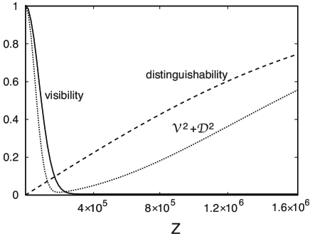
Figure 3: Visibility and distingishability vs charge for the parameters of Ref. tonomura , for which the characteristic charge $Z_{1}$ for distinguishing paths by measuring the Coulomb field is $\sim 7\times 10^{5}$, and the characteristic charge $Z_{2}$ for loss of interference is $\sim 1.5\times 10^{5}$. Also shown is $\mathcal{V}^{2}+\mathcal{D}^{2}$ (dotted line).

A simple interpretation of the decrease in visibility, in terms of the Aharonov-Bohm effect aharonov-bohm , is that the closed electron loop, $u-l$, encircles a fluctuating electromagnetic field which shifts the interference pattern randomly, thus tending to wash it out. The interpretation of the reduction of the pattern in terms of a random flux requires photon emission processes, and is equivalent to the present discussion. Indeed, for the subset of processes in which there is no photon emission, the modification of the interference pattern is given by $\langle U_{l}^{\dagger}\rangle\langle U_{u}\rangle$ [cf. (16)], where the brackets denote states with zero photons. Now

$${\rm Re}\log\langle U_{u}\rangle=-\frac{Z^{2}\alpha}{3\pi}\int kdk\left|\oint_{u}e^{-i\omega t}\vec{v}(t)\right|^{2}\simeq\frac{1}{4}\log{\cal V};$$ (32)

the reduction reflects the loss of forward-scattering amplitude owing to photon emission processes. Thus, the zero-photon emission pattern is multiplied by a factor ${\cal V}^{1/2}$; the suppression of the zero-photon pattern at charge $\sqrt{2}Z$ equals the suppression of the total visibility at charge $Z$. The phase of $\langle U_{l}^{\dagger}\rangle\langle U_{u}\rangle$ is essentially proportional to the difference of real parts of the electron self-energy corrections on the upper and lower paths, corrections that do not contribute to the diminution of the interference pattern.

III Measuring the path by gravity

Finally, we ask if it is possible to detect the path by measuring the fluctuations in the (Newtonian) gravitational potential at large distance as a particle of sufficiently large mass passes through the slits. In this scenario, the Newtonian gravitational field plays the role of the Coulomb field for charged particles. We consider detecting the change of the Newtonian gravitational field by using a modern gravity wave detector, e.g., a highly sensitive laser interferometer HRS (a measurement not equivalent to detecting possible gravitational radiation produced by the mass going through the slits). Figure 4 sketches such a detector. As before, the x-axis lies in the plane of the slits. We assume that the mirrors in the detector are tied down in the lab frame; to a first approximation, the distance between the mirrors (or equivalently the ends of a Weber bar) is a harmonic degree of freedom, with oscillator frequency, $\omega$ (which includes the gravitational attraction of the two mirrors).

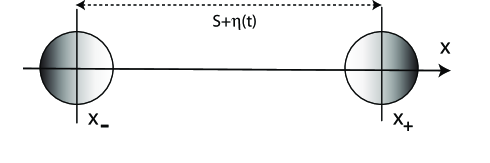
Figure 4: Gravitational field detector

We derive schematically the response of the detector to a Newtonian gravitational potential $\phi(x,t)$. In the presence of $\phi$, the positions of the mirrors, $x_{\pm}$, obey the Newtonian equations of motion,

$$\frac{\partial^{2}x_{\pm}}{\partial t^{2}} =\mp\frac{1}{2}\omega^{2}[x_{+}(t)-x_{-}(t)-S]-\phi^{\prime}(x_{\pm}),$$ (33)

with $S$ the equilibrium distance between the mirrors, and the prime denoting differentiation with respect to $x$. We write $x_{\pm}=x_{0}\pm(S+\eta)/2$, where $x_{0}$ is the midpoint between the mirrors in equilibrium, and $\eta$ is the relative displacement of the mirrors caused by the gravitational pulse. Then linearizing in $\eta$ and $\phi^{\prime\prime}$ we have

$$\frac{\partial^{2}\eta(t)}{\partial t^{2}}=-\omega\eta(t)-\phi^{\prime\prime}(x_{0})S.$$ (34)

For simplicity we assume that $\phi$ is zero before the gravitational pulse reaches the detector, and is constant in time during the detection. With initial conditions $\eta(0)=\eta^{\prime}(0)=0$, we obtain

$$\eta(t)=-\phi^{\prime\prime}(x_{0})S\frac{1-\cos\omega t}{\omega^{2}}.$$ (35)

The accuracy required for the measurement of $\phi^{\prime\prime}(x_{0})$ is

$$\Delta\phi^{\prime\prime}(x_{0})=2Gm\left(\frac{1}{R^{3}}-\frac{1}{(R+d)^{3}}\right)\sim\frac{Gmd}{R^{4}},$$ (36)

where $m$ is the mass of the particle, and the measuring apparatus, as before, is at a distance $R$ from the slits. Thus, since $1-\cos\omega t\leq(\omega t)^{2}/2$, one needs to measure $\eta$ to an accuracy,

$$\Delta\eta\mathrel{\hbox to0.0pt{\raise 2.20013pt\hbox{$<$}\hss}{\lower 2.20013pt\hbox{$\sim$}}}\frac{GmdST^{2}}{R^{4}}<\frac{Gmd}{Rc^{2}},$$ (37)

which implies that the mass scale for which one can begin to distinguish the path obeys,

$$\frac{Gm^{2}}{\hbar c}\mathrel{\hbox to0.0pt{\raise 2.20013pt\hbox{$>$}\hss}{\lower 2.20013pt\hbox{$\sim$}}}\left(\frac{\Delta\eta}{\ell_{\rm pl}}\right)^{2}\left(\frac{R}{d}\right)^{2}.$$ (38)

Physically the uncertainty $\Delta\eta$ must exceed the Planck length footnote5 , and thus

$$\frac{Gm^{2}}{\hbar c}\mathrel{\hbox to0.0pt{\raise 2.20013pt\hbox{$>$}\hss}{\lower 2.20013pt\hbox{$\sim$}}}\left(\frac{R}{d}\right)^{2};$$ (39)

the mass scale must be a factor $R/d$ larger than the Planck mass, $\sqrt{\hbar c/G}\sim 2\times 10^{-5}$ g. For $R/d\sim 6\times 10^{4}$ tonomura , the scale would have to be of order 1 g.

The interference pattern caused by a particle whose mass obeys the condition (39) has a fringe separation,

$$\delta_{f}\sim\frac{L}{d}\frac{\hbar}{mv}\mathrel{\hbox to0.0pt{\raise 2.20013pt\hbox{$<$}\hss}{\lower 2.20013pt\hbox{$\sim$}}}\ell_{\rm pl}\frac{cT}{R}\mathrel{\hbox to0.0pt{\raise 2.20013pt\hbox{$<$}\hss}{\lower 2.20013pt\hbox{$\sim$}}}\ell_{\rm pl},$$ (40)

which implies that when the mass is large enough to allow which-path detection via gravity, the pattern becomes immeasurably fine, of order the Planck length or shorter. This result assures the consistency of quantum mechanics; however, unlike in the electromagnetic case, consistency does not require that the gravitational field be quantized footnote6 . (Although a decrease of the visibility of the pattern would arise were gravity quantized, as in the electromagnetic situation, detailed calculations of the diminution would depend on the detailed theory of quantized gravity assumed, an issue we do not address here.)

In summary, when one can distinguish the path of a particle by measuring the electromagnetic or gravitational field at large distance, interference disappears. For large enough charge on the interfering particle, emission of quantized electromagnetic radiation destroys the interference, while for large enough mass, the pattern becomes too fine to be discerned.

- (1) Aage Petersen, private communication to G. Baym, Copenhagen ca. 1961. Petersen was Niels Bohr’s scientific secretary (amanuensis) from 1952 until Bohr’s death in 1962.
- (2) Tonomura A, Endo J, Matsuda T, Kawasaki T, and Ezawa H (1989) Demonstration of single-electron buildup of an interference pattern. Am. J. Phys. 57, 117-120.
- (3) To the authors knowledge, this experiment is not mentioned in Bohr’s published papers, unpublished manuscripts, or letters. Aage Bohr, when queried about the experiment, wrote that, “Many ways of observing effects distinguishing between the “paths” of the electron were certainly discussed … I do not remember any specific scheme exploiting the Coulomb field far away from the electron.” (Letter to G. Baym, 6 June 2001.) References to N. Bohr’s ideas in this paper follow Petersen’s description of the experiment. We are grateful to Felicity Pors of the Niels Bohr Archives of the Niels Bohr Institute in Copenhagen for her generous archival assistance.
- (4) Bohr N and Rosenfeld L (1933) Zur Frage der Messbarkeit der elektromagnetischen Feldgrössern. Mat.-fys. Medd. Dansk Vid. Selsk. 12, No. 8. [Engl. transl. (1996) in Niels Bohr Collected Works, v. 7, ed Kalckar J (North-Holland Publ. Co., Amsterdam) p123].
- (5) Bohr N and Rosenfeld L (1950) Field and charge measurements in quantum electrodynamics. Phys. Rev. 78, 794-798.
- (6) Aharonov Y and Bohm D (1959) Significance of electromagnetic potentials in the quantum theory. Phys. Rev. 115, 485-491.
- (7) Aharonov Y and Popescu S, unpublished; P. Kwiat, private communication.
- (8) Grangier P, Roger G, and Aspect A (1986) Experimental evidence for a photon anticorrelation effect on a beam splitter: a new light on single-photon interferences. Europhys. Lett. 1 173-179.
- (9) Pfau T, Spälter S, Kurtsiefer Ch, Ekstrom CR, and Mlynek J (1994) Loss of spatial coherence by a single spontaneous emission. Phys. Rev. Lett. 73, 1223-1226.
- (10) Chapman MS et al. (1995) Photon scattering from atoms in an atom interferometer: coherence lost and regained, Phys. Rev. Lett. 75, 3783-3787.
- (11) Scully MO, Englert B-G, and Walther H (1991) Quantum optical tests of complementarity. Nature 351, 111-116.
- (12) Furry WH and Ramsey NF (1960) Significance of Potentials in Quantum Theory. Phys. Rev. 118, 623-626.
- (13) Olariu S and Iovitzu Popescu I (1985) The quantum effects of electromagnetic fluxes. Rev. Mod. Phys. 57, 339-436.
- (14) Stern A, Aharonov Y, and Imry Y (1990) Phase uncertainty and loss of interference: A general picture. Phys. Rev. A 41, 3436-3448.
- (15) Schuster R et al. (1997) Phase measurement in a quantum dot via a double-slit interference experiment. Nature 385, 417-420.
- (16) Buks E, Schuster R, Heiblum M, Mahalu D, and Umansky V (1998) Dephasing in electron interference by a ’which-path’ detector. Nature 391, 871-874.
- (17) Chang D-I et al. (2008) Quantum mechanical complementarity probed in a closed-loop Aharonov-Bohm interferometer. Nature Physics 4, 205-209.
- (18) Calmet X, Graesser M, and Hsu SDH (2004) Minimum length from quantum mechanics and classical general relativity. Phys. Rev. Lett. 93, 211101.
- (19) Landau L and Peierls RE (1931) Erweiterung des Unbestimmtheitsprinzips für die relavistische Quantentheorie. Z. f. Phys. 69, 56-69.
- (20) Compagno G and Persico F (1998) Limits of the measurability of the local quantum electromagnetic-field amplitude. Phys. Rev. A 57, 1595-1603.
- (21) Hnizdo V (1999) Comment on limits of the measurability of the local quantum electromagnetic-field amplitude. Phys. Rev. A 60, 4191-4195.
- (22) Saavedra LGP (2004) Quantum control, entanglement and noise in the seminal Bohr and Rosenfeld paper on electromagnetic field measurements. AIP Conf. Proc. 734, 75-78.
- (23) Wootters WK and Zurek WH (1978) Complementarity in the double-slit experiment: Quantum nonseparability and a quantitative statement of Bohr’s principle. Phys. Rev. D 19, 473-484.
- (24) Jaeger G, Shimony A, and Vaidman L (1994) Two interferometric complementarities. Phys. Rev. A 51, 54-67.
- (25) Englert B-G (1996) Fringe visibility and which-way information: an inequality. Phys. Rev. Lett. 77, 2154-2157.
- (26) Jacques V et al. (2008) Delayed-choice test of quantum complementarity with interfering single photons. Phys. Rev. Lett. 100, 220402.
- (27) Wilson KG (1974) Confinement of quarks. Phys. Rev. D 10, 2445-2459.
- (28) Ford LH (1992) Electromagnetic vacuum fluctuations and electron coherence. Phys. Rev. D 47, 5571-5580.
- (29) Breuer H and Petruccione F (2001) Destruction of quantum coherence through emission of bremsstrahlung. Phys. Rev. A 63, 032102.
- (30) Note that emission of photons with wavelengths larger than the slit width contributes to the decrease in visibility, even though such photons give little or no information about the path. The reason is that photon emission leads to fragmentation of the total amplitude, , among photon states with various numbers of photons, . Here . Only states and with the same photon state can interfere; the total weight of the interfering terms must be .
- (31) Hough J, Rowan S, and Sathyaprakash BS (2005) The search for gravitational waves. J. Phys. B: At. Mol. Opt. Phys. 38 S497-S519.
- (32) When the displacement is measured by the difference of measured relative positions of the mirrors at times and , a first estimate of the accuracy of the measurement of is the standard quantum limit , where is the mass of each mirror, The mirrors cannot be arbitrarily massive, since the apparatus cannot form a black hole peresrosen , so that , and consequently the standard quantum limit implies, . Various ways to improve on this simple limit using techniques such as contractive state measurements yuen ; ozawa , or quantum nondemolition measurements qndrevmodphys ; braginsky have been proposed. However, our result is independent of these details.
- (33) Peres A and Rosen N (1960) Quantum limitations on the measurement of gravitational fields. Phys. Rev. 118, 335-336.
- (34) Yuen HP (1983) Contractive States and the Standard Quantum Limit for Monitoring Free-Mass Positions. Phys. Rev. Lett. 51, 719-722.
- (35) Ozawa M (1988) Measurement breaking the standard quantum limit for free-mass position. Phys. Rev. Lett. 60, 385-388.
- (36) Caves CM, Thorne KS, Drever RWP, Sandberg VD, and Zimmermann M (1980) On the measurement of a weak classical force coupled to a quantum-mechanical oscillator. I. Issues of principle. Rev. Mod. Phys. 52, 341-392.
- (37) Braginsky VB et al. (2003) Noise in gravitational-wave detectors and other classical-force measurements is not influenced by test-mass quantization. Phys. Rev. D 67, 082001.
- (38) As in the electromagnetic case, one expects a crossover with increasing mass from indistinguishable to distinguishable paths. However, a better understanding of the nature of space-time on the Planck scale is required to determine a quantitivative visibility.