Cooling and squeezing the fluctuations of a nanomechanical beam by indirect quantum feedback control

Abstract

We study cooling and squeezing the fluctuations of a nanomechanical beam using quantum feedback control. In our model, the nanomechanical beam is coupled to a transmission line resonator via a superconducting quantum interference device (SQUID). The leakage of the electromagnetic field from the transmission line resonator is measured using homodyne detection. This measured signal is then used to design a quantum-feedback-control signal to drive the electromagnetic field in the transmission line resonator. Although the control is imposed on the transmission line resonator, this quantum-feedback-control signal indirectly affects the thermal motion of the nanomechanical beam via the inductive beam-resonator coupling, making it possible to cool and squeeze the fluctuations of the beam, allowing it to approach the standard quantum limit.

I Introduction

Nanomechanical oscillators have recently attracted considerable attention for their possible applications in quantum information and quantum measurement (see, e.g., Refs. Schwab ; Blencowe ; Ekinci ; Cleland ; Buks1 ; Sergey1 ; Mancini ; Mahboob ; Wei ; Marshall ; Huang ; Gaidarzhy ; Metzger ; Naik ; Gigan ; Arcizet ; Schliesser ; Kippenberg ; Corbitt ; Bhattacharya ; Kleckner ; Cohadon ; Poggio ; Schliesser2 ; Rae ; Marquardt ; Genes ; YDWang ; MGrajcar ; LTian ; Naik2 ; Hopkins ; Rae2 ). A nanomechanical oscillator is also a promising device for studying macroscopic quantum effects in mechanical systems (see, e.g., Refs. Schwab ; Blencowe ; Ekinci ; Cleland ; Buks1 ; Sergey1 ; Mancini ; Mahboob ; Wei ; Marshall ). Using current experimental techniques (see, e.g., Refs. Ekinci ; Huang ; Gaidarzhy ), high-frequency nanomechanical oscillators ($\omega/2\pi\sim 1$ GHz) with quality factors $Q$ in the range of $10^{3}$–$10^{5}$ can be realized at low temperatures $T$ on the order of mK. When the vibrational energy $\hbar\omega$ of the nanomechanical oscillator becomes smaller than the thermal energy $k_{B}T$, the oscillator can be said to work in the quantum regime.

To observe quantum behavior in nanomechanical oscillators, e.g., quantum fluctuations or squeezing effects, the oscillator must be cooled to extremely low temperatures to approach the standard quantum limit. There have been numerous studies, both theoretical and experimental (see, e.g., Refs. Metzger ; Naik ; Gigan ; Arcizet ; Schliesser ; Kippenberg ; Corbitt ; Bhattacharya ; Kleckner ; Cohadon ; Poggio ; Schliesser2 ; Rae ; Marquardt ; Genes ; YDWang ; MGrajcar ; LTian ; Naik2 ; Hopkins ; Rae2 ; Ouyang ; Martin ; PZhang ; You ; Hauss ; Vinante ; Xue ; Teufel ), investigating the cooling of the fluctuations of nanomechanical oscillators. Many of these studies focus on optomechanical systems (see, e.g., Refs. Metzger ; Naik ; Gigan ; Arcizet ; Schliesser ; Kippenberg ; Corbitt ; Bhattacharya ; Kleckner ; Cohadon ; Poggio ), where an oscillating cantilever or an oscillating micro-mirror is modelled as a harmonic oscillator. There are two approaches in optomechanical cooling: passive cooling Metzger ; Naik ; Gigan ; Arcizet ; Schliesser ; Kippenberg ; Corbitt ; Bhattacharya and active cooling Kleckner ; Cohadon ; Poggio . In passive cooling techniques, the mechanical oscillator is self-cooled by the dynamical back-action, e.g., the radiation-pressure-induced back-action Naik ; Gigan ; Arcizet ; Schliesser ; Kippenberg ; Corbitt ; Bhattacharya coming from the mirror surface of the optical cavity. In fact, for a high-finesse cavity, the photons reflected from the mirror of the cavity transfer momentum and induce additional damping to the mechanical oscillator. In active cooling techniques, the reflected signal coming from the mechanical oscillator is sent to an electronic circuit, e.g., a derivative circuit, to provide a modulating signal, which is then used to control the back-action force imposed on the mechanical oscillator. Since the cooling effect can be actively controlled by tuning the feedback gain obtained in the control circuit, this is called an active cooling strategy.

Although it has recently been reported that ground-state cooling Schliesser2 ; Rae ; Marquardt ; Genes could be realized in optomechanical systems, it is difficult to observe the macroscopic quantum effects of the mechanical oscillators in these optomechanical systems using current experimental conditions. The main difficulty comes from the fact that the characteristic oscillating frequency of the mechanical oscillator in these systems is not high enough (typically on the order of kHz or MHz), and the corresponding effective temperature to observe the quantum effects is extremely low (typically on the order of nK or $\mu$K), which is difficult to realize in present-day experiments.

Besides optomechanical cooling, a nanomechanical oscillator can also be embedded in an electronic circuit and cooled by coupling it to an electronic system YDWang ; MGrajcar ; LTian . Possible strategies include nanomechanical oscillators coupled to superconducting single-electron transistors Naik2 ; Hopkins , quantum dots Rae2 ; Ouyang , Josephson-junction superconducting circuits Martin ; PZhang ; You ; Hauss ; Vinante , or transmission line resonators Xue ; Teufel . Compared with mechanical oscillators in optical systems, a high-frequency oscillator can be realized more easily in electronic systems. Indeed, it has been reported that nanomechanical beams Huang ; Gaidarzhy with frequencies in the regime of GHz have been realized, and these beams seem to be suitable for integration in an electronic circuit. Since the effective temperature of such a mechanical oscillator can be in the mK regime, it should be possible to observe quantum behavior in this case.

Like optomechanical systems, active feedback controls can be introduced to cool the motions of the nanomechanical oscillators in electronic systems. In the theoretical proposal in Ref. Hopkins , a nanomechanical resonator is capacitively coupled to a single-electron transistor to measure the position of the resonator. The information obtained by the quantum measurement is fed into a feedback circuit to obtain an output control signal, which is then imposed on a feedback electrode to control the motion of the resonator. In this strategy, the quantum measurement and the designed feedback control introduce additional damping effects on the resonator, which are helpful for cooling the motion of the resonator.

In a recent experiment Etaki , a nanomechanical beam acted as one side of a superconducting quantum interference device (SQUID), and the voltage across the SQUID was measured which can be used to detect the motion of the beam. Motivated by this experiment, here we study the coupling between such a system Etaki and a transmission line resonator. A single-mode quantized electromagnetic field provided by this resonator You2 could be detected by a homodyne measurement Blais . The quantization of this coupled beam–SQUID–resonator system has been addressed in the literature (see, e.g., Ref. Buks2 ; Buks3 ; Buks4 ), and theoretical analysis shows that such a device can be used to detect the motion of the beam Buks4 . Here, we would like to concentrate on a different problem: how to design a quantum feedback control from the output signal of the homodyne detection to drive the motion of the beam? Different from previous work, such as the one in Ref. Hopkins , the quantum feedback control proposed here is imposed on the transmission line resonator, not on the beam, and indirectly controls the motion of the nanomechanical beam via the coupling between the transmission line resonator and the beam. By adiabatically eliminating the degrees of freedom of the SQUID and the transmission line resonator, the designed feedback control could introduce anharmonic terms in the effective Hamiltonian and additional damping terms for the nanomechanical beam, leading to both cooling and squeezing of the fluctuations of the beam.

This paper is organized as follows: in Sec. II, we present a coupled system composed of: (i) a transmission line resonator, (ii) an rf-SQUID, and (iii) a nanomechanical beam. The open quantum system model and the quantum weak measurement approach used to design the feedback control are investigated in Sec. III. The quantum feedback control design is presented in Sec. IV, and our main results about squeezing and cooling the fluctuations of the beam are discussed in Sec. V. The conclusion and discussion of possible future work are presented in Sec. VI.

II System model and Hamiltonian

We mainly focus on a physical model in which a doubly-clamped nanomechanical beam, a rf-SQUID, and a transmission line resonator are inductively coupled (see, e.g., Ref. Buks2 ; Buks3 ; Buks4 ). The quantum electromechanical circuit and the corresponding equivalent schematic diagram are shown in Fig. 1. In this circuit, the mechanical oscillator, i.e., the clamped nanomechanical beam, is integrated into the rf-SQUID with a Josephson junction having a critical current $I_{c}$ and a capacitance $C$. Here, the displacement of the beam in the plane of the loop with a small amplitude $x$ around its equilibrium position changes the area of the loop, and thus influences the total magnetic flux $\Phi$ threading the loop. There is an applied external flux $\Phi_{e}$ threading the loop. The rf-SQUID interacts with a nearby transmission line resonator (TLR), via their mutual inductance. The additional magnetic flux provided by the quantized current in the transmission line resonator is

$$\Phi_{\rm add}=\Phi_{T}(-ia+ia^{\dagger}),$$

where $\Phi_{T}$ is a constant; $a$ and $a^{\dagger}$ are the annihilation and creation operators of the quantized electromagnetic field in the transmission line resonator. Here, we ignore the small change of $\Phi_{T}$ caused by the oscillation of the beam. For this superconducting circuit, the total magnetic flux $\Phi$ threading the loop of the rf-SQUID is given by:

$$\Phi=\Phi_{e}+Blx+\Phi_{T}(-ia+ia^{\dagger})+LI,$$

where $L$ and $I$ are, respectively, the self-inductance and the current in the loop; $l$ is the effective length of the beam; and $B$ is the magnetic field threading the loop of the rf-SQUID at the location of the nanomechanical beam, and is assumed to be constant in the region where the beam oscillates.

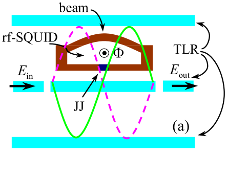
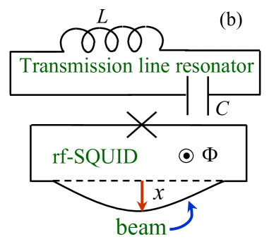
Figure 1: (color online) (a) Schematic diagram of a transmission line resonator (TLR), in blue, and a SQUID-nanomechanical beam system, in beige and dark blue. Here, “JJ” represents a Josephson junction, and $E_{\rm in}$, $E_{\rm out}$ are, respectively, the input and output electromagnetic fields of the transmission line resonator. (b) Diagram of the quantum circuit.

The total Hamiltonian of this coupled electromechanical system can be written as Buks3 :

$$H=H_{0}+H_{1},$$ (1)

with the Hamiltonians:

$$H_{0} = \frac{p^{2}}{2m}+\frac{m\omega_{M}^{2}x^{2}}{2}+\hbar\,\omega_{T}a^{\dagger}a+\hbar\,u(t)(a^{\dagger}+a),$$ (2)

$$H_{1} = U_{0}\left[\phi-\phi_{e}-\kappa(-ia+ia^{\dagger})-\frac{2\pi Bl}{\Phi_{0}}x\right]^{2}$$ (3)

$$+2U_{0}\beta_{L}\cos\phi+\frac{q^{2}}{2C},$$

where $\Phi_{0}$ is the flux quantum; $\omega_{M}$ is the oscillating frequency of the doubly-clamped beam; $\phi$ and $\phi_{e}$ are related to the normalized total flux and external flux:

$$\phi=2\pi\left(\frac{\Phi}{\Phi_{0}}-\frac{1}{2}\right),\quad\phi_{e}=2\pi\left(\frac{\Phi_{e}}{\Phi_{0}}-\frac{1}{2}\right).$$

The normalized system parameters $U_{0}$, $\beta_{L}$ and $\kappa$ in Eq. (1) are given by:

$$U_{0} = \frac{\Phi_{0}^{2}}{8\pi L},\quad\beta_{L}=\frac{2\pi LI_{c}}{\Phi_{0}},\quad\kappa=\frac{2\pi\Phi_{T}}{\Phi_{0}}.$$

The observables $p$ and $q$ in Eqs. (2) and (3) are, respectively, the conjugate observables of $x$ and $\Phi$ representing the momentum of the beam and the charge on the Josephson junction. The term $\hbar u(t)(a^{\dagger}+a)$ in Eq. (2) is an interaction Hamiltonian between the transmission line resonator and the external control field, where the time-dependent function $u(t)$ can be designed according to the desired goal.

When $\beta_{L}>1$ and

$$\left|\phi_{e}+\frac{2\pi Blx}{\Phi_{0}}+\kappa(-ia+ia^{\dagger})\right|=|\phi_{e}^{\prime}|\ll 1,$$ (4)

the Hamiltonian $H_{1}$ represents a double-well potential near $\phi=0$, and the two lowest eigenstates, $|L\rangle$ and $|R\rangle$, correspond to two current states with opposite circulating currents in the loop of the rf-SQUID, which are far separated from higher-energy eigenstates. At sufficiently low temperatures, only the two lowest eigenstates $|L\rangle$, $|R\rangle$ contribute. Thus, the rf-SQUID can be modelled as a two-level system, and the Hamiltonian $H_{1}$ of the rf-SQUID can be re-expressed as Buks3 :

$$H_{1}=\frac{\hbar\,\epsilon}{2}\left(\phi_{e}+\frac{2\pi Bl}{\Phi_{0}}x+\kappa(-ia+ia^{\dagger})\right)\tilde{\sigma}_{z}-\frac{\hbar\,\Delta}{2}\tilde{\sigma}_{x},$$

where $\tilde{\sigma}_{x}$ and $\tilde{\sigma}_{z}$ are the $x$-axis and $z$-axis Pauli operators in the basis of $|L\rangle$ and $|R\rangle$; $\epsilon$, $\Delta$ are real parameters that determine the energy difference between the two minima of the double-well potential and the tunnelling amplitude between the wells, respectively. Under the condition that

$$0<\left(\beta_{L}-1\right)\ll 1,$$

then $\epsilon$ and $\Delta$ can be approximately given by RMigliore :

$$\epsilon=\frac{I_{c}\Phi_{0}}{\hbar\pi}\sqrt{6(\beta_{L}-1)},\quad\Delta=3U_{0}\left(1-\frac{1}{\beta_{L}}\right)^{2}.$$ (5)

Letting the external flux $\phi_{e}=0$, we can rewrite the Hamiltonian $H_{1}$ in the qubit basis as:

$$H_{1}=\frac{\hbar\,\omega_{S}}{2}\sigma_{z}+\frac{\hbar\,\pi\epsilon Bl}{\Phi_{0}}x\sigma_{x}+\frac{\hbar\,\kappa\epsilon}{2}(-ia+ia^{\dagger})\sigma_{x},$$ (6)

where $\omega_{S}=\Delta$, and $\sigma_{x}$, $\sigma_{z}$ are the corresponding $x$-axis and $z$-axis Pauli operators in the qubit basis:

$$|+\rangle = \frac{\sqrt{2}}{2}|L\rangle+\frac{\sqrt{2}}{2}|R\rangle,$$

$$|-\rangle = \frac{\sqrt{2}}{2}|L\rangle-\frac{\sqrt{2}}{2}|R\rangle.$$

Here, we assume that the oscillation frequency of the beam is high enough such that $\omega_{M}$, $\omega_{S}$, and $\omega_{T}$ are comparable. Then, under the rotating-wave approximation, and with Eq. (6), the total Hamiltonian in Eq. (1) becomes:

$$H = \frac{\hbar\,\omega_{S}}{2}\sigma_{z}+\hbar\,\omega_{M}b^{\dagger}b+\hbar\,\omega_{T}a^{\dagger}a$$ (7)

$$+\hbar\,u(t)(a^{\dagger}+a)+\hbar\,g_{MS}(b\sigma_{+}+\sigma_{-}b^{\dagger})$$

$$+\hbar\,g_{ST}(-ia\sigma_{+}+i\sigma_{-}a^{\dagger}),$$

where the coupling strength $g_{MS}$ between the mechanical oscillator and the rf-SQUID is:

$$g_{MS}=g_{\rm Mech-SQUID}=\frac{\pi\epsilon Bl}{\Phi_{0}\sqrt{2\hbar\,m\omega_{M}}},$$

and the coupling strength $g_{ST}$ between the rf-SQUID and the transmission line resonator is given by:

$$g_{ST}=g_{\rm SQUID-TLR}=\frac{\kappa\epsilon}{2\hbar}.$$

The annihilation and creation operators $b$ and $b^{\dagger}$ of the fundamental oscillating mode of the nanomechanical beam are defined by:

$$b = \sqrt{\frac{m\omega_{M}}{2\hbar}}x+i\frac{1}{\sqrt{2\hbar\,m\omega_{M}}}p,$$

$$b^{\dagger} = \sqrt{\frac{m\omega_{M}}{2\hbar}}x-i\frac{1}{\sqrt{2\hbar\,m\omega_{M}}}p.$$

Furthermore, let us assume that the frequencies of the rf-SQUID, the beam, and the transmission line resonator satisfy the conditions:

$$g_{MS}\ll\Delta_{MS}=\omega_{S}-\omega_{M},\quad g_{ST}\ll\Delta_{ST}=\omega_{S}-\omega_{T}.$$ (8)

Then, in this large-detuning regime CPSun , the following transformation can be introduced to diagonalize the Hamiltonian $H$ in Eq. (7):

$$U=\exp\left[\frac{g_{MS}}{\Delta_{MS}}(b\sigma_{+}-b^{\dagger}\sigma_{-})-\frac{g_{ST}}{\Delta_{ST}}(ia\sigma_{+}+ia^{\dagger}\sigma_{-})\right].$$

In fact, under the condition given in Eq. (8), we can obtain an effective Hamiltonian:

$$H_{\rm eff} = UHU^{\dagger}$$

$$\approx \hbar\,\omega_{M}b^{\dagger}b+\hbar\,\omega_{T}a^{\dagger}a+\hbar\,u(t)(a^{\dagger}+a)$$

$$+\frac{\hbar\omega_{S}}{2}\sigma_{z}+\hbar\left(\frac{g_{MS}^{2}}{\Delta_{MS}}b^{\dagger}b+\frac{g_{ST}^{2}}{\Delta_{ST}}a^{\dagger}a\right)\sigma_{z}$$

$$+\hbar\left(\frac{g_{MS}g_{ST}}{\Delta_{MS}}+\frac{g_{MS}g_{ST}}{\Delta_{ST}}\right)(-iba^{\dagger}+ib^{\dagger}a)\sigma_{z},$$

by expanding $UHU^{\dagger}$ to first order in $g_{MS}/\Delta_{MS}$ and $g_{ST}/\Delta_{ST}$.

III Interaction between the system and its environment

A real physical system inevitably interacts with the external degrees of freedom in the environment. Such interactions introduce noise to the system. There are three kinds of noise that should be considered here: the thermal noises on the nanomechanical beam and the transmission line resonator, as well as the electromagnetic fluctuations on the rf-SQUID caused by the nearby electromagnetic elements.

The interaction Hamiltonians between the transmission line resonator, the beam, the rf-SQUID and their environments can be described as:

$$H_{\rm int}^{(1)} = (a+a^{\dagger})X_{\rm bath}^{(1)},$$

$$H_{\rm int}^{(2)} = (b+b^{\dagger})X_{\rm bath}^{(2)},$$

$$H_{\rm int}^{(3)} = (M_{\phi}\sigma_{z}+M_{r}\sigma_{x})X_{\rm bath}^{(3)},$$

where $X_{\rm bath}^{(1)}$, $X_{\rm bath}^{(2)}$ and $X_{\rm bath}^{(3)}$ are, respectively, the environmental operators interacting with the transmission-line resonator, the beam and the rf-SQUID; $M_{\phi}$ and $M_{r}$ are two constants which determine the dephasing and relaxation rates of the rf-SQUID. Furthermore, let us consider a bosonic model of the environment, and assume that the interactions between the system degrees of freedom and the environmental degrees of freedom are linear interactions. Then, under the rotating-wave approximation and the Markovian approximation, we can obtain the following quantum stochastic differential equation for a system observable $X$ (see Appendix A for the derivation):

$$dX = -\frac{i}{\hbar}[X,H_{\rm eff}]dt+\frac{\gamma_{S}}{2}M_{\phi}^{2}[\sigma_{z},[X,\sigma_{z}]]$$ (9)

$$+\frac{\gamma_{S}}{2}M_{r}^{2}\left(\sigma_{+}[X,\sigma_{-}]+[\sigma_{+},X]\sigma_{-}\right)$$

$$+\frac{\gamma_{M}}{2}(\bar{n}_{M}+1)\left(b^{\dagger}[X,b]+[b^{\dagger},X]b\right)$$

$$+\frac{\gamma_{M}}{2}\bar{n}_{M}\left(b[X,b^{\dagger}]+[b,X]b^{\dagger}\right)$$

$$+\frac{\gamma_{T}}{2}\left(a^{\dagger}[X,a]+[a^{\dagger},X]a\right)$$

$$+\sqrt{\eta\gamma_{T}}dA_{\rm in}^{\dagger}[X,a]+\sqrt{\eta\gamma_{T}}[a^{\dagger},X]dA_{\rm in},$$

where $\gamma_{M}$, $\gamma_{S}$, $\gamma_{T}$ are the damping rates of the mechanical beam, the rf-SQUID and the transmission line resonator under the Markovian approximation;

$$\bar{n}_{M}=\frac{1}{e^{\hbar\omega_{M}/k_{B}T}-1}$$ (10)

is the average photon number of the beam in thermal equilibrium with the environment at temperature $T$. To simplify our discussions, when Eq. (9) was derived, we neglected environment-induced thermal excitations on the transmission line resonator and the rf-SQUID (these excitations could indeed be neglected with the parameters given in Eqs. (V.1) and (V.1) in Sec. V). The leakage of the transmission line resonator could be detected using a homodyne detection with detection efficiency $\eta$, where $dA_{\rm in}$ represents a quantum Wiener noise Gardiner satisfying:

$$dA_{\rm in}^{\dagger}dA_{\rm in}=dA_{\rm in}dA_{\rm in}=dA_{\rm in}^{\dagger}dA_{\rm in}^{\dagger}=0,$$

$$dA_{\rm in}dA_{\rm in}^{\dagger}=dt.$$

Here, we only keep the fluctuation terms caused by the measurement and average over the other fluctuations, because the evolution of the coupled beam-SQUID-resonator system is conditioned on the measurement output, which depends on the measurement-induced fluctuations. The corresponding measurement output of the homodyne detection can be expressed as Buks4 :

$$dY_{t}=\sqrt{\eta\gamma_{T}}(a^{\dagger}+a)+\left(dA_{\rm in}+dA_{\rm in}^{\dagger}\right).$$ (11)

Note that this measurement output depends on the input noise and the electromagnetic field of the transmission line resonator.

IV Quantum filtering and quantum feedback control

There are two possible ways to design a quantum feedback control protocol Mabuchi ; Jacobs1 based on the measurement output. One approach is to directly feed back the output signal to design the quantum feedback control signal, which leads to the Markovian quantum feedback control Wiseman1 . Another approach, which is called quantum Bayesian feedback control Doherty1 , can be divided into two steps: the first step is to find a so-called quantum filtering equation Belavkin ; Bouten ; NYamamoto1 to give an estimate of the state of the system from the measurement output; the second step is to design a feedback control signal based on the estimated state. The possibility for a “control problem” to be divided into these two steps, i.e., a separate filtering step and a control step, is called the separation principle in control theory, which has recently been developed for quantum control systems Bouten . Compared with the Markovian quantum feedback control, the quantum Bayesian feedback control can be applied to more general systems. In our proposal, we will design the control using Bayesian feedback control.

Based on quantum filtering theory, which has been well developed in the literatures Belavkin ; Bouten , we can obtain the following stochastic master equation for the estimated state $\tilde{\rho}$:

$$d\tilde{\rho} = -\frac{i}{\hbar}[H_{\rm eff},\tilde{\rho}]dt+\gamma_{M}\bar{n}_{M}\mathcal{D}\left[b^{\dagger}\right]\tilde{\rho}dt$$ (12)

$$+\gamma_{M}\left(\bar{n}_{M}+1\right)\mathcal{D}[b]\tilde{\rho}dt+\gamma_{S}M_{\phi}^{2}\mathcal{D}[\sigma_{z}]\tilde{\rho}dt$$

$$+\gamma_{S}M_{r}^{2}\mathcal{D}[\sigma_{-}]\tilde{\rho}dt+\gamma_{T}\mathcal{D}[a]\tilde{\rho}dt$$

$$+\sqrt{\eta\gamma_{T}}\mathcal{H}[a]\tilde{\rho}\left(dY_{t}-\sqrt{\eta\gamma_{T}}\langle\left(a^{\dagger}+a\right)\rangle dt\right),$$

where

$$\tilde{\rho}=E(\rho|\mathcal{Y}_{t})$$ (13)

is defined as the conditional expectation of the density operator $\rho$ for the coupled beam-SQUID-resonator system under the von Neumann algebra Bouten :

$$\mathcal{Y}_{t}={vN}\left\{Y_{s}|t_{0}\leq s\leq t\right\},$$ (14)

spanned by the measurement outputs; $\langle A\rangle={\rm tr}(A\tilde{\rho})$ is the average of $A$ under $\tilde{\rho}$; and the superoperators $\mathcal{D}[c]\tilde{\rho}$ and $\mathcal{H}[c]\tilde{\rho}$ are defined by:

$$\mathcal{D}[c]\tilde{\rho} = c\tilde{\rho}c^{\dagger}-\frac{1}{2}c^{\dagger}c\tilde{\rho}-\frac{1}{2}\tilde{\rho}c^{\dagger}c,$$

$$\mathcal{H}[c]\tilde{\rho} = c\tilde{\rho}+\tilde{\rho}c^{\dagger}-\langle\left(c+c^{\dagger}\right)\rangle\tilde{\rho}.$$

The increment

$$dW=dY_{t}-\sqrt{\eta\gamma_{T}}\langle\left(a^{\dagger}+a\right)\rangle dt$$ (15)

in Eq. (12) is the innovation updated by the quantum measurement, which has been proved to be a classical Wiener increment satisfying:

$$E(dW)=0,\quad(dW)^{2}=dt.$$

for homodyne detection (see, e.g., Ref. Bouten ).

The von Neumann algebra $\mathcal{Y}_{t}$ defined in Eq. (14) represents the information obtained by the quantum measurement up to time $t$; thus the conditional expectation $\tilde{\rho}$ defined in Eq. (13) is the best estimate of the system’s state obtained from the measurement output.

Generally, the stochastic master equation, i.e., the filter equation, is difficult to solve. However, for the system we discuss here, the stochastic master equation (12) is equivalent to a set of closed equations under the semiclassical approximation (see Eqs. (B) and (B) in Appendix B). This set of equations can be integrated by a Data Acquisition Processor (DAP) (see, e.g., Ref. Mabuchi ), which is composed of a Digital Signal Processor (DSP) and analog/digital and digital/analog signal converters. Such a Data Acquisition Processor works as an integral estimator of the dynamics of the system state and gives the output signals $\langle x_{T}\rangle$ and $\langle p_{T}\rangle$. The output signals of the estimator are fed into a feedback controller (a linear amplification element) to obtain the following feedback control signal:

$$u(t)=\sqrt{\frac{2}{\hbar}}\left(-\upsilon_{x}\langle x_{T}\rangle+\upsilon_{p}\langle p_{T}\rangle\right),$$ (16)

where $\upsilon_{x}$ and $\upsilon_{p}$ are the feedback control gains that can be chosen according to the desired goal, and $x_{T}$, $p_{T}$ are the normalized position and momentum operators of the transmission line resonator defined by:

$$x_{T}=\sqrt{\frac{\hbar}{2}}\left(a^{\dagger}+a\right),\quad p_{T}=\sqrt{\frac{\hbar}{2}}\left(-ia+ia^{\dagger}\right).$$ (17)

We replace $u(t)$ in Eq. (9) and Eq. (12) by Eq. (16) to obtain new dynamical equations. In this case, we indeed control, simultaneously, the evolutions of the transmission line resonator and the estimator. The schematic diagram of the feedback control circuit is shown in Fig. 2. From the definition (13) of $\tilde{\rho}$, it can be shown that the control of the coupled system given by Eq. (9) is equivalent to the control of the estimator given by Eq. (12). Thus, in the following discussion, we will focus on how to control the quantum filtering equation (12).

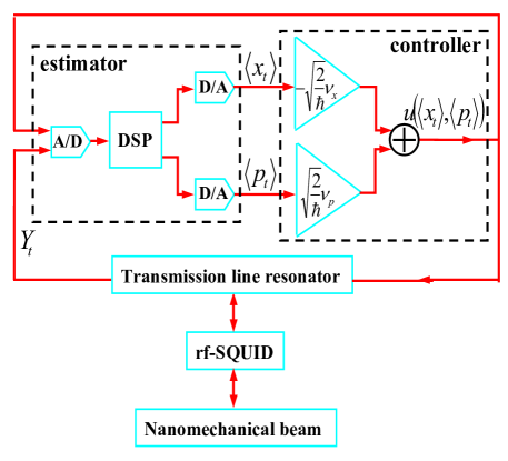
Figure 2: (color online) Schematic diagram of the feedback control circuit. The “DSP” denotes a Digital Signal Processor (DSP) which works as the integral estimator of the system state by solving Eqs. (B) and (B). The “A/D” and “D/A” represent the analog/digital and digital/analog signal converters. The output of the estimator is fed into a linear amplifier circuit to obtain a control signal which is further used to drive the input electromagnetic field of the transmission line resonator and the input of the estimator.

If the damping rates $\gamma_{S}$ and $\gamma_{T}$ of the rf-SQUID and the transmission line resonator are large enough such that

$$\gamma_{S},\,\gamma_{T}\gg\gamma_{M}\bar{n}_{M},$$ (18)

we can adiabatically eliminate Walls ; Steck the degrees of freedom of the rf-SQUID and the transmission line resonator to obtain the following reduced stochastic master equation and the measurement output for the nanomechanical beam (see Appendix B for the derivation):

$$d\tilde{\rho}_{M} = -\frac{i}{\hbar}[H^{(M)}_{\rm eff},\tilde{\rho}_{M}]dt+\gamma_{M}\bar{n}_{M}\mathcal{D}[b^{\dagger}]\tilde{\rho}_{M}dt$$

$$+\gamma_{M}(\bar{n}_{M}+1)\mathcal{D}[b]\tilde{\rho}_{M}dt$$

$$+\gamma_{T}\mathcal{D}[C_{1}b+C_{2}b^{\dagger}]\tilde{\rho}_{M}dt$$

$$+\sqrt{\eta\gamma_{T}}\mathcal{H}[C_{1}b+C_{2}b^{\dagger}]\tilde{\rho}_{M}dW,$$

$$dY_{t} = \sqrt{\eta\gamma_{T}}\langle\left(\alpha_{x}b+\alpha_{x}^{*}b^{\dagger}\right)\rangle dt+dW,$$ (19)

where the reduced Hamiltonian $H^{(M)}_{\rm eff}$ is given by:

$$H^{(M)}_{\rm eff} = \hbar\,\omega_{M}b^{\dagger}b+\hbar\,\xi_{M}b^{2}+\hbar\,\xi_{M}^{*}b^{\dagger\,2}$$ (20)

$$+\hbar\,\tilde{u}(t)(\alpha_{x}b+\alpha_{x}^{*}b^{\dagger}),$$

and the reduced effective control on the beam is:

$$\tilde{u}(t) = -\upsilon_{x}\langle\left(\alpha_{x}b+\alpha_{x}^{*}b^{\dagger}\right)\rangle+\upsilon_{p}\langle\left(\alpha_{p}b+\alpha_{p}^{*}b^{\dagger}\right)\rangle.$$

The parameters $\alpha_{x}$, $\alpha_{p}$, $\xi_{M}$ can be expressed as:

$$\alpha_{x} = C_{1}+C_{2}^{*},$$

$$\alpha_{p} = -iC_{1}+iC_{2}^{*},$$

$$\xi_{M} = \omega_{T}C_{2}^{*}C_{1}-ig_{MT}C_{2}^{*},$$

where $g_{MT}$ is given by Eq. (39) and $C_{1}$, $C_{2}$ are given by:

$$C_{1}\left(v_{x},v_{p}\right) = \frac{g_{MT}}{\chi}\left[\left(\upsilon_{p}+\frac{\gamma_{T}}{2}\right)-i(-\upsilon_{x}+\omega_{T})\right],$$

$$C_{2}\left(v_{x},v_{p}\right) = \frac{g_{MT}}{\chi}(\upsilon_{p}-i\upsilon_{x}),$$

$$\chi\left(v_{x},v_{p}\right) = \frac{\gamma_{T}}{4}(\gamma_{T}+4\upsilon_{p})+\omega_{T}(\omega_{T}-2\upsilon_{x}).$$ (21)

As shown in Eq. (20), there is a two-photon term $\hbar\xi_{M}b^{2}+\hbar\xi_{M}^{*}b^{\dagger\,2}$ in the effective Hamiltonian $H_{\rm eff}^{(M)}$, which leads to squeezing in the fluctuations of the beam. Without the quantum feedback control, i.e., $\upsilon_{x}=\upsilon_{p}=0$, $\xi_{M}$ would be zero and the two-photon term vanishes.

Equation (IV) shows that the quantum measurement and feedback control introduce extra damping and fluctuation terms for the beam (the third and fourth lines in Eq. (IV)). These damping terms are important for squeezing and cooling the fluctuations of the beam.

V Squeezing and cooling the fluctuations of the nanomechanical beam

In order to study the squeezing and cooling effects on the nanomechanical beam induced by the quantum feedback control, let us first define the normalized position and momentum operators of the nanomechanical beam:

$$x_{M}=\sqrt{\frac{\hbar}{2}}(b+b^{\dagger}),\quad p_{M}=\sqrt{\frac{\hbar}{2}}(-ib+ib^{\dagger}).$$

Then, from the reduced stochastic master equation (IV), we can study the evolutions and the corresponding stationary values of the variances

$$V_{x_{M}}=\langle x_{M}^{2}\rangle-\langle x_{M}\rangle^{2},\quad V_{p_{M}}=\langle p_{M}^{2}\rangle-\langle p_{M}\rangle^{2}$$ (22)

of $x_{M}$ and $p_{M}$.

V.1 Squeezing

The nanomechanical beam can be described by the conjugate variables $x_{M}$ and $p_{M}$, and is in a squeezed state if the corresponding variances of these variables defined in Eq. (22) satisfy $V_{x_{M}}<\hbar/2$ or $V_{p_{M}}<\hbar/2$, i.e., the variance of one of the two conjugate variables is below the standard quantum limit (see, e.g., Refs. Hu ; Hu2 ; Zagoskin ). Owing to the uncertainty principle which requires that $V_{x_{M}}V_{p_{M}}\geq\hbar^{2}/4$, squeezing the fluctuations of one of the two conjugate variables would lead to the dispersion of the fluctuations of the other conjugate variable.

If we choose the feedback control gains $\upsilon_{x}$ and $\upsilon_{p}$ to satisfy the conditions

$$0 < \frac{\gamma_{T}}{\gamma_{T}+4\upsilon_{p}}\ll 1,$$

$$0 < \frac{\omega_{T}-2\upsilon_{x}}{\omega_{T}}\ll 1,$$

$$0 < \frac{\gamma_{T}g_{MT}^{2}\omega_{T}^{2}}{\omega_{M}}\ll\chi^{2},$$ (23)

then the stationary variances $V^{c}_{x_{M}}$ and $V^{c}_{p_{M}}$ can be estimated as:

$$V_{x_{M}}^{c}\approx\frac{\hbar}{2}\sqrt{\frac{\xi}{\eta}},\quad V_{p_{M}}^{c}\approx\frac{\hbar}{2}\frac{1}{\sqrt{\xi\eta}},$$ (24)

where

$$\xi=\frac{\omega_{M}-2{\rm Re}\,\xi_{M}}{\omega_{M}+2{\rm Re}\,\xi_{M}},\quad{\rm Re}\,\xi_{M}\approx\frac{\omega_{T}g^{2}_{MT}}{\chi^{2}}(\upsilon_{p}^{2}-\upsilon_{x}^{2}).$$ (25)

It is shown in Eq. (24) that the parameter $\xi$ determines the tradeoff of the squeezing effects between $V_{x_{M}}$ and $V_{p_{M}}$. When $\xi>1$, the fluctuation of the momentum $p_{M}$ of the nanomechanical beam is squeezed. However, when $\xi<1$, the fluctuation of the position $x_{M}$ of the nanomechanical beam is squeezed. The parameter $\eta$, i.e., the measurement efficiency of the homodyne detection, determines the minimum uncertainty that can be reached. For a quantum weak measurement with a high efficiency $\eta$ such that

$$\frac{1}{(2\bar{n}_{M}+1)^{2}}<\eta<1,$$

where $\bar{n}_{M}$ is the thermal excitation number of the beam given in Eq. (10), it can be verified that

$$\frac{\hbar^{2}}{4} < V_{x_{M}}^{c}V_{p_{M}}^{c}\approx\frac{\hbar^{2}}{4\eta}$$

$$< V_{x_{M}}^{uc}V_{p_{M}}^{uc}=\hbar^{2}\left(\bar{n}_{M}+\frac{1}{2}\right)^{2},$$

where $V^{uc}_{x_{M}}$ and $V^{uc}_{p_{M}}$ are the “uncontrolled” stationary variances that are obtained from Eq. (IV) by letting $\upsilon_{x}=\upsilon_{p}=0$. It should be pointed out that the product of the uncertainties of $x_{M}$ and $p_{M}$ given by Eq. (24), i.e.,

$$V_{x_{M}}^{c}V_{p_{M}}^{c}\approx\frac{\hbar^{2}}{4\eta},$$

corresponds to the Heisenberg uncertainty limit of a quantum system under imperfect quantum weak measurements (see, e.g., Ref. NYamamoto2 ). When the measurement efficiency $\eta$ tends to unity, the traditional Heisenberg uncertainty limit $\hbar^{2}/4$ is recovered.

To show the validity of our strategy, let us show some numerical examples. The system parameters are chosen as Buks3 :

$$L=3.38\times 10^{-11}\,\,{\rm H},\quad C=7.4\times 10^{17}\,\,{\rm F},$$

$$I_{c}=10\,\,{\rm\mu A},\quad m=10^{-16}\,\,{\rm kg},\quad\eta=0.6,$$

$$\omega_{M}/2\pi=1\,\,{\rm GHz},\quad Bl=1\,\,{\rm T}\times{\rm\mu m},$$

$$Q=10^{4},\quad T=100\,\,{\rm mK},\quad\phi_{e}=0,$$

$$\gamma_{S}/2\pi=100\,\,{\rm MHz},\quad\gamma_{T}/2\pi=20\,\,{\rm MHz},$$

$$g_{ST}/2\pi=20\,\,{\rm MHz},\quad\omega_{T}/2\pi=4.3\,\,{\rm GHz}.$$ (26)

From the above parameters, it can be calculated that

$$\gamma_{M}/2\pi\approx 0.1\,\,{\rm MHz},\quad\omega_{S}/2\pi\approx 6.3\,\,{\rm GHz}$$

$$g_{MS}/2\pi\approx 73\,\,{\rm MHz},\quad g_{MT}/2\pi\approx 4.9\,\,{\rm MHz}.$$ (27)

In our numerical results, the stationary variances are calculated from the dynamic equation (IV), and the feedback control parameters $\upsilon_{x}$ and $\upsilon_{p}$ are chosen to satisfy Eq. (V.1). In fact, in Fig. 3, we choose $\upsilon_{x}$ and $\upsilon_{p}$ such that

$$\upsilon_{x}=0.5\,\omega_{T},\quad 0.5\leq\frac{\upsilon_{p}}{\omega_{T}}\leq 1.$$ (28)

In this case, we have $\upsilon_{p}^{2}\geq\upsilon_{x}^{2}$. Then, from Eqs. (24) and (25), it can be verified that $V_{x_{M}}^{c}\leq V_{p_{M}}^{c}$, which coincides with the numerical results in Fig. 3(a) (the blue dashed line for $V_{x_{M}}^{c}/\hbar$ is below the green triangular line for $V_{p_{M}}^{c}/\hbar$). It means that the fluctuation of the position of the beam is squeezed. Meanwhile, the numerical results in Fig. 3(b) show that the variances $V_{x_{M}}^{c}$ and $V_{p_{M}}^{c}$ under control are much smaller than the variances $V_{x_{M}}^{uc}$ and $V_{p_{M}}^{uc}$ without control, which means that the designed feedback control reduces the variances of the position and momentum of the beam. The product of the variances under control $V_{x_{M}}^{c}V_{p_{M}}^{c}$ could even be reduced to be close to the Heisenberg uncertainty limit $\hbar^{2}/4$.

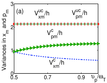
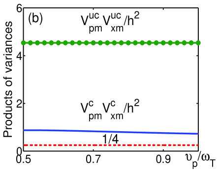
Figure 3: (color online) Squeezing the position-fluctuations of the beam with the parameters given in Eqs. (V.1), (V.1), and (28). (a) Variances of the position and momentum of the beam (in units of $\hbar$) versus the normalized control parameter $\tilde{\upsilon}_{p}=\upsilon_{p}/\omega_{T}$. Recall that $\upsilon_{p}$ is the linear feedback gain (see, Eq. (16)). The green line with triangles and the blue dashed line represent, respectively, the controlled variances of the position $V_{x_{M}}^{c}/\hbar$ and momentum $V_{p_{M}}^{c}/\hbar$ of the beam. The red line with asterisks and the blue solid line represent the uncontrolled variances $V_{x_{M}}^{uc}/\hbar$ and $V_{p_{M}}^{uc}/\hbar$ of the beam, which coincide because the beam without control is in a coherent thermal state with equal variances of position and momentum. (b) Products of the variances (in units of $\hbar^{2}$) versus the normalized control parameter $\tilde{\upsilon}_{p}=\upsilon_{p}/\omega_{T}$. The green line with asterisks and the blue solid line denote the uncontrolled trajectory $V_{x_{M}}^{uc}V_{p_{M}}^{uc}/\hbar^{2}$ and the controlled trajectory $V_{x_{M}}^{c}V_{p_{M}}^{c}/\hbar^{2}$, respectively. The red dashed line at $1/4$ represents the Heisenberg uncertainty limit $\hbar^{2}/4$.

In Fig. 4, we choose $\upsilon_{x}$ and $\upsilon_{p}$ such that

$$\upsilon_{x}=0.5\,\omega_{T},\quad 0.3\leq\frac{\upsilon_{p}}{\omega_{T}}\leq 0.5.$$ (29)

In this case, we can calculate from Eqs. (24) and (25) that $V_{x_{M}}^{c}\geq V_{p_{M}}^{c}$, which coincides with the numerical results in Fig. 4(a) (the green triangular line for $V_{p_{M}}^{c}/\hbar$ is below the blue dashed line for $V_{x_{M}}^{c}/\hbar$). It means that the fluctuations of the momentum of the beam are squeezed. More interestingly, the numerical results in Fig. 4(a) show that the variance of $p_{M}$ is squeezed to be less than the standard quantum limit, i.e., $V_{p_{M}}^{c}<\hbar/2$. Numerical results in Fig. 4(b) show that the product $V_{x_{M}}^{c}V_{p_{M}}^{c}$ of the controlled variances is much smaller than the product $V_{x_{M}}^{uc}V_{p_{M}}^{uc}$ of the uncontrolled variances, which means that the variances of the position and momentum of the beam could be reduced under the designed feedback control. Indeed, as shown in Fig. 4(b), the product of the variances could be reduced to be close to the Heisenberg uncertainty limit $\hbar^{2}/4$.

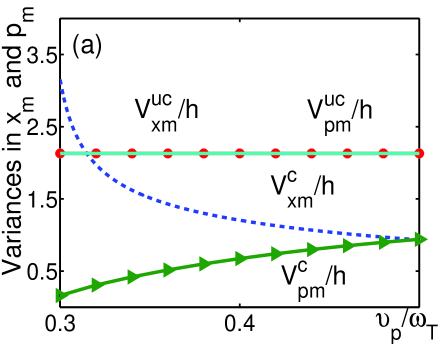
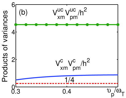
Figure 4: (color online) Squeezing the momentum-fluctuations of the beam with the parameters given in Eqs. (V.1), (V.1), and (29). (a) Variances of the position and momentum of the beam (in units of $\hbar$) versus the normalized control parameter $\tilde{\upsilon}_{p}=\upsilon_{p}/\omega_{T}$. The green line with triangles and the blue dashed line represent, respectively, the controlled variances of the position $V_{x_{M}}^{c}/\hbar$ and momentum $V_{p_{M}}^{c}/\hbar$ of the beam. The red line with asterisks and the blue solid line represent the uncontrolled variances $V_{x_{M}}^{uc}/\hbar$ and $V_{p_{M}}^{uc}/\hbar$ of the beam, which coincide because the beam without control is in a coherent thermal state with equal variances of position and momentum. (b) Products of the variances (in units of $\hbar^{2}$) versus the normalized control parameter $\tilde{\upsilon}_{p}=\upsilon_{p}/\omega_{T}$. The green line with asterisks and the blue solid line denote the uncontrolled trajectory $V_{x_{M}}^{uc}V_{p_{M}}^{uc}/\hbar^{2}$ and the controlled trajectory $V_{x_{M}}^{c}V_{p_{M}}^{c}/\hbar^{2}$, respectively. The red dashed line at $1/4$ represents the Heisenberg uncertainty limit $\hbar^{2}/4$.

V.2 Cooling

Further, let us investigate the cooling of the fluctuations of the nanomechanical beam. The cooling effect can be estimated by the average photon number of the nanomechanical beam

$$\bar{n} = E_{dW}(\langle b^{\dagger}b\rangle)$$ (30)

$$= \frac{1}{2\hbar}(V_{x_{M}}+V_{p_{M}})-\frac{1}{2}+\frac{1}{2\hbar}(V_{\langle x_{M}\rangle}+V_{\langle p_{M}\rangle})$$

$$+\frac{1}{2\hbar}(\bar{x}_{M}^{2}+\bar{p}_{M}^{2}),$$

with

$$\bar{x}_{M}=E_{dW}(\langle x_{M}\rangle),\quad\bar{p}_{M}=E_{dW}(\langle p_{M}\rangle),$$

$$V_{\langle x_{M}\rangle}=E_{dW}(\langle x_{M}\rangle^{2})-\bar{x}_{M}^{2},$$

$$V_{\langle p_{M}\rangle}=E_{dW}(\langle p_{M}\rangle^{2})-\bar{p}_{M}^{2}.$$

Here, $E_{dW}$ means that the expectations and variances of $\langle x_{M}\rangle$ and $\langle p_{M}\rangle$ are about the Wiener noise $dW$.

From the system parameters given in Eqs. (V.1) and (V.1), it can be verified that the controlled stationary expectations $\bar{x}_{M}^{c}$, $\bar{p}_{M}^{c}$ and the classical fluctuations $V^{c}_{\langle x_{M}\rangle}$, $V^{c}_{\langle p_{M}\rangle}$ satisfy

$$\bar{x}_{M}^{c}=\bar{p}_{M}^{c}=0,\quad V_{\langle x_{M}\rangle}^{c}\ll V_{x_{M}}^{c},\quad V_{\langle p_{M}\rangle}^{c}\ll V_{p_{M}}^{c}.$$

Thus, from Eqs. (24) and (30), the controlled stationary average photon number can be estimated as:

$$\bar{n}^{c} \approx \frac{1}{2\hbar}(V_{x_{M}}^{c}+V_{p_{M}}^{c})-\frac{1}{2}$$ (31)

$$\approx \frac{1}{4}\left(\sqrt{\frac{\xi}{\eta}}+\frac{1}{\sqrt{\xi\eta}}\right)-\frac{1}{2},$$

which, under the parameters given in Eqs. (V.1), (V.1), (28), and (29), is smaller than the uncontrolled stationary average photon number

$$\bar{n}^{uc}\approx\frac{1}{2\hbar}(V_{x_{M}}^{uc}+V_{p_{M}}^{uc})-\frac{1}{2}\approx\bar{n}_{M},$$

where $\bar{n}_{M}$ is given in Eq. (10).

Alternatively, we can use an effective temperature $T_{\rm eff}$ to quantify the cooling effect which is defined by:

$$\bar{n}=\frac{1}{e^{\hbar\omega_{M}/k_{B}T_{\rm eff}}-1},$$

or, equivalently,

$$T_{\rm eff}=\frac{\hbar\omega_{M}}{k_{B}\ln\left(\frac{\bar{n}+1}{\bar{n}}\right)}.$$ (32)

The controlled stationary effective temperature $T_{\rm eff}^{c}$ can be estimated as follows:

$$T_{\rm eff}^{c}\approx\frac{\hbar\omega_{M}}{k_{B}\ln\left(\frac{\sqrt{\xi/\eta}+\sqrt{1/\xi\eta}+2}{\sqrt{\xi/\eta}+\sqrt{1/\xi\eta}-2}\right)}.$$ (33)

We now give some physical interpretations of our cooling strategy. There are two competing processes that determine the stationary effective temperature of the nanomechanical beam. The cooling process is provided by the leakage of the transmission line resonator, whose energy gap is larger than $k_{B}T$ such that the thermal excitation from the environment could be negligible. Energy flows from the beam to the transmission line resonator via the coupling between them, and then it is dissipated via the leakage of the transmission line resonator. An opposing heating process is provided by the thermal excitation of the beam from the environment. Without applying quantum feedback control on the transmission line resonator, the cooling process of the beam is weak compared with the heating process, which leads to the failure of cooling. When we apply quantum feedback control and adjust the control parameters to be in the region given by Eq. (V.1), the decay of the beam caused by the leakage from the transmission line resonator is enhanced to overwhelm the heating process. Thus, the nanomechanical beam is effectively cooled.

To show the validity of our proposal, let us show some numerical examples. The system parameters are chosen as in Eqs. (V.1) and (V.1), and the feedback control parameters $\upsilon_{x}$ and $\upsilon_{p}$ are chosen such that

$$\upsilon_{x}=0.5\,\omega_{T},\quad 0.3\leq\frac{\upsilon_{p}}{\omega_{T}}\leq 1.$$ (34)

The numerical results in Fig. 5 show that the average photon number and the effective temperature of the beam under control are reduced compared with the uncontrolled case. It means that our strategy can indeed effectively cool the motion of the beam. With the parameters given in Eqs. (V.1), (V.1), and (34), the minimum average photon number that can be reached is about $0.43$ (corresponding to an effective temperature $T_{\rm eff}^{c}\approx 6.3$ mK). Further calculations show that, if we increase $\upsilon_{p}/\omega_{T}$ further, the minimum average photon number that can be reached by our strategy is about $0.35$ (corresponding to an effective temperature $T_{\rm eff}^{c}\approx 5.6$ mK).

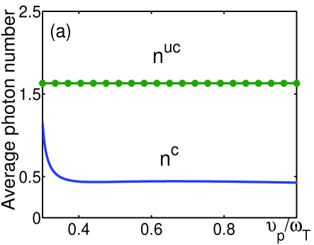
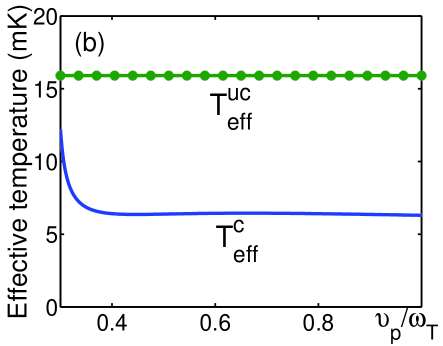
Figure 5: (color online) Cooling the nanomechanical beam for (a) the average photon number $\bar{n}$, and (b) the effective temperature $T_{\rm eff}$ versus the normalized control parameter $\tilde{\upsilon}_{p}=\upsilon_{p}/\omega_{T}$. The blue solid lines representing the average photon number $n^{c}$ and effective temperature $T_{\rm eff}^{c}$ under control are below the green lines with asterisks representing the corresponding average photon number $n^{uc}$ and effective temperature $T_{\rm eff}^{uc}$ without control, which means that the designed feedback control could effectively cool the fluctuations of the beam induced by thermal noises.

VI Conclusions

In summary, we have investigated the possibility of using quantum feedback control to squeeze and cool down the fluctuations of a nanomechanical beam embedded in a coupled transmission line resonator–SQUID–mechanical beam quantum circuit. The leakage of the electromagnetic field from the transmission line resonator is detected using homodyne measurement, and the measurement output is then used to design a quantum-feedback-control signal to drive the electromagnetic field in the transmission line resonator. The designed quantum-feedback-control protocol indirectly affects the motion of the beam by the inductive coupling between the transmission line resonator and the beam via the rf- SQUID. After adiabatically eliminating the degrees of freedom of the rf-SQUID and the transmission line resonator, the quantum feedback control results in a two-photon term in the effective Hamiltonian and additional damping terms for the beam, which lead to squeezing and cooling for the beam. By varying the feedback control parameters, the variance of either the position or momentum of the beam could be squeezed, and the variance of the momentum of the beam could even be squeezed to be less than the standard quantum limit $\hbar/2$. Meanwhile, the average photon number (or, equivalently, the effective temperature) of the beam could be reduced effectively by applying control, compared with the uncontrolled case.

Although the thermal motion of the beam could be effectively suppressed by the proposed quantum feedback control protocol, our calculations show that the beam has not achieved the ground state. Further work will focus on extending our results to explore ways to further lower the achievable effective temperature or even attain the ground state of the beam. Another possible direction is to consider nonlinear effects Jacobs2 of the nanomechanical oscillator, which may affect the achievable cooling temperature and the squeezing effects induced by the quantum feedback control.

ACKNOWLEDGMENTS

We thank Dr. S. Ashhab for his great help on this work. J. Zhang would like to thank Dr. N. Yamamoto for helpful discussions. FN acknowledges partial support from the National Security Agency (NSA), Laboratory Physical Science (LPS), Army Research Office (ARO), National Science Foundation (NSF) grant No. EIA-0130383, JSPS-RFBR 06-02-91200. J. Zhang was supported by the National Natural Science Foundation of China under Grant Nos. 60704017, 60635040, 60674039 and the China Postdoctoral Science Foundation.

Appendix A Derivation of the quantum stochastic differential equation (9)

Consider a bosonic model of the environmental degrees of freedom, and assume that the interactions between the degrees of freedom of the system and the environmental ones have linear interactions. Then, under the rotating-wave approximation, the Hamiltonian of the total system, composed of the degrees of freedom of the system and the environment, can be expressed as:

$$H_{\rm tot} = H_{\rm eff}+\int\hbar\omega c_{pT}^{\dagger}c_{pT}d\omega+\int\hbar\omega c_{eT}^{\dagger}c_{eT}d\omega$$

$$+\int\hbar\omega c_{eM}^{\dagger}c_{eM}d\omega+\int\hbar\omega c_{eS}^{\dagger}c_{eS}d\omega$$

$$+\hbar\int d\omega\left[g_{pT}^{*}(\omega)c^{\dagger}_{pT}a+g_{pT}(\omega)a^{\dagger}c_{pT}\right]$$

$$+\hbar\int d\omega\left[g_{eT}^{*}(\omega)c^{\dagger}_{eT}a+g_{eT}(\omega)a^{\dagger}c_{eT}\right]$$

$$+\hbar\int d\omega\left[g_{eM}^{*}(\omega)c^{\dagger}_{eM}b+g_{eM}(\omega)b^{\dagger}c_{eM}\right]$$

$$+\hbar M_{\phi}\int d\omega\left[g_{eS}^{*}(\omega)c^{\dagger}_{eS}\sigma_{z}+g_{eS}(\omega)\sigma_{z}c_{eS}\right]$$

$$+\hbar M_{r}\int d\omega\left[g_{eS}^{*}(\omega)c^{\dagger}_{eS}\sigma_{-}+g_{eS}(\omega)\sigma_{+}c_{eS}\right],$$

where $c_{pT}$ ($c_{pT}^{\dagger}$), $c_{eT}$ ($c_{eT}^{\dagger}$), $c_{eM}$ ($c_{eM}^{\dagger}$), $c_{eS}$ ($c_{eS}^{\dagger}$) are, respectively, the annihilation (creation) operators of different environmental degrees of freedom, which satisfy

$$[c_{i}(\omega),c_{j}^{\dagger}(\omega^{\prime})]=\delta_{ij}\delta(\omega-\omega^{\prime}).$$

The subscripts “pT” and “eT” represent the environmental degrees of freedom interacting with the transmission line resonator being “probed” (pT) and not being probed (eT). The subscripts “eM” and “eS” denote the environmental (thus the “e”) degrees of freedom interacting with the mechanical beam and the SQUID, respectively.

Let $X$ be a system operator, then the Heisenberg equation for $X$ can be written as:

$$dX = -\frac{i}{\hbar}[X,H_{\rm tot}dt]-\frac{1}{2\hbar^{2}}[[X,H_{\rm tot}dt],H_{\rm tot}dt]$$

$$= -\frac{i}{\hbar}[X,H_{\rm eff}]dt+d\,L_{pT}(X)+dL_{eT}(X)$$

$$+dL_{eM}(X)+dL_{eS,\,\varphi}(X)+dL_{eS,\,r}(X),$$

where

$$dL_{\alpha}(X)=-\frac{i}{\hbar}[X,H_{\alpha}dt]-\frac{1}{2\hbar^{2}}[[X,H_{\alpha}dt],H_{\alpha}dt],$$

and

$$H_{pT} = \hbar\int d\omega\left[g_{pT}^{*}(\omega)c_{pT}^{\dagger}a+g_{pT}(\omega)a^{\dagger}c_{pT}\right],$$

$$H_{eT} = \hbar\int d\omega\left[g_{eT}^{*}(\omega)c_{eT}^{\dagger}a+g_{eT}(\omega)a^{\dagger}c_{eT}\right],$$

$$H_{eM} = \hbar\int d\omega\left[g_{eM}^{*}(\omega)c_{eM}^{\dagger}b+g_{eM}(\omega)b^{\dagger}c_{eM}\right],$$

$$H_{eS,\varphi} = \hbar M_{\phi}\int d\omega\left[g_{eS}^{*}(\omega)c_{eS}^{\dagger}\sigma_{z}+g_{eS}(\omega)\sigma_{z}c_{eS}\right],$$

$$H_{eS,r} = \hbar M_{r}\int d\omega\left[g_{eS}^{*}(\omega)c_{eS}^{\dagger}\sigma_{-}+g_{eS}(\omega)\sigma_{+}c_{eS}\right].$$

Here, we expand $dX$ to second-order differential terms, because we may meet quantum Wiener increments and the second-order terms cannot be omitted.

In order to eliminate the environmental degrees of freedom corresponding to $c_{pT}(\omega)$, we first solve the equation for $c_{pT}(\omega)$:

$$\dot{c}_{pT}(\omega)=-\frac{i}{\hbar}[c_{pT}(\omega),H_{\rm tot}]=-i\omega\,c_{pT}(\omega)-ig_{pT}^{*}(\omega)a$$

to obtain

$$c_{pT}(\omega,t) = \int_{t_{0}}^{t}dt^{\prime}e^{-i\omega(t-t^{\prime})}(-ig^{*}_{pT}(\omega))a(t^{\prime})$$ (36)

$$+e^{-i\omega(t-t_{0})}c_{pT}(\omega,t_{0}).$$

Further, let us introduce the so-called first Markovian approximation to omit the frequency dependence of the coupling strength Buks2 :

$$g_{pT}(\omega)=\sqrt{\frac{\gamma_{pT}}{2\pi}}e^{i\phi_{pT}},$$ (37)

where $\gamma_{pT}$ and $\phi_{pT}$ are independent of $\omega$.

By substituting Eqs. (36) and (37) into $dL_{pT}(X)$, we have

$$-\frac{i}{\hbar}[X,H_{pT}dt] = \left\{\int d\omega|g_{pT}(\omega)|^{2}\int_{t_{0}}^{t}dt^{\prime}e^{-i\omega(t-t^{\prime})}\right.$$

$$\left.(a^{\dagger}(t^{\prime})[X,a]+a(t^{\prime})[a^{\dagger},X])\right\}dt$$

$$-ig^{*}_{pT}\int d\omega e^{i\omega(t-t_{0})}c^{\dagger}_{pT}(\omega,t_{0})[X,a]dt$$

$$+ig_{pT}[a^{\dagger},X]\int d\omega e^{-i\omega(t-t_{0})}c_{pT}(\omega,t_{0})dt$$

$$= \frac{\gamma_{pT}}{2}\left(a^{\dagger}[X,a]-a[X,a^{\dagger}]\right)dt$$

$$+\left(-i\sqrt{\gamma_{pT}}e^{-i\phi_{pT}}d\tilde{A}_{\rm in}^{\dagger}\right)[X,a]$$

$$+[a^{\dagger},X]\left(i\sqrt{\gamma_{pT}}e^{i\phi_{pT}}d\tilde{A}_{\rm in}\right),$$

where

$$d\tilde{A}_{\rm in}=\left(\frac{1}{\sqrt{2\pi}}\int d\omega e^{-i\omega(t-t_{0})}c_{pT}(\omega,t_{0})\right)dt$$

is the input quantum noise such that

$$d\tilde{A}_{\rm in}d\tilde{A}_{\rm in}^{\dagger}=(\bar{n}(\omega_{T})+1)dt,$$

$$d\tilde{A}_{\rm in}^{\dagger}d\tilde{A}_{\rm in}=\bar{n}(\omega_{T})dt,$$

$$d\tilde{A}_{\rm in}d\tilde{A}_{\rm in}=d\tilde{A}_{\rm in}^{\dagger}d\tilde{A}_{\rm in}^{\dagger}=0,$$

and

$$\bar{n}(\omega)=\frac{1}{e^{\hbar\omega/k_{B}T}-1}.$$

Further, we have

$$-\frac{1}{2\hbar^{2}}[[X,H_{pT}dt],H_{pT}dt] = -\frac{\gamma_{pT}}{2}\bar{n}(\omega_{T})[[X,a],a^{\dagger}]dt$$

$$-\frac{\gamma_{pT}}{2}(\bar{n}(\omega_{T})+1)[[X,a^{\dagger}],a]dt.$$

From the above analysis, it can be calculated that

$$d\,L_{pT}(X) = -\frac{i}{\hbar}[X,H_{pT}dt]-\frac{1}{2\hbar^{2}}[[X,H_{pT}],H_{pT}dt]$$

$$= \frac{\gamma_{pT}}{2}(\bar{n}(\omega_{T})+1)\left(a^{\dagger}[X,a]+[a^{\dagger},X]a\right)$$

$$+\frac{\gamma_{pT}}{2}\bar{n}(\omega_{T})\left(a[X,a^{\dagger}]+[a,X]a^{\dagger}\right)$$

$$+\sqrt{\gamma_{pT}}dA_{\rm in}^{\dagger}[X,a]+\sqrt{\gamma_{pT}}[a^{\dagger},X]dA_{\rm in},$$

where $dA_{\rm in}=ie^{i\phi_{pT}}d\tilde{A}_{\rm in}$.

With the same analysis, we can calculate $dL_{eT}(X)$, $dL_{eM}(X)$, $dL_{eS,\varphi}(X)$, and $dL_{eS,r}(X)$. Furthermore, under the condition that $\hbar\omega_{S},\hbar\omega_{T}\gg k_{B}T$, we have $\bar{n}(\omega_{S}),\,\bar{n}(\omega_{T})\approx 0$. Thus, by substituting the above results into Eq. (A), averaging over the fluctuations caused by the thermal noises, and assuming that

$$\gamma_{T}=\gamma_{pT}+\gamma_{eT},\quad\eta=\frac{\gamma_{pT}}{\gamma_{pT}+\gamma_{eT}},$$

we can obtain the quantum stochastic differential equation (9).

In order to calculate the measurement output of the homodyne detection, let us recall that the input and output detection noises should be

$$d\tilde{A}_{\rm in} = \left(\frac{1}{\sqrt{2\pi}}\int d\omega e^{-i\omega(t-t_{0})}c_{pT}(\omega,t_{0})\right)dt,$$

$$d\tilde{A}_{\rm out} = \left(\frac{1}{\sqrt{2\pi}}\int d\omega e^{-i\omega(t-t_{0})}c_{pT}(\omega,t_{1})\right)dt,$$

where the time $t_{0}$ is an instant before the measurement commences, and the time $t_{1}$ is another instant after the measurement has finished. The measurement output is related to $d\tilde{A}_{\rm out}$ by:

$$dY_{t}=e^{-i\phi_{LO}}d\tilde{A}_{\rm out}^{\dagger}+e^{i\phi_{LO}}d\tilde{A}_{\rm out},$$

where $\phi_{LO}$ is an adjustable phase introduced by the local oscillator of the homodyne detection. From Eq. (36), we have

$$c_{pT}(\omega,t) = -i\sqrt{\gamma_{pT}}e^{-i\phi_{pT}}\frac{1}{\sqrt{2\pi}}\int_{t_{0}}^{t}dt^{\prime}e^{-i\omega(t-t^{\prime})}a(t^{\prime})$$

$$+e^{-i\omega(t-t_{0})}c_{pT}(\omega,t_{0})$$

$$= -i\sqrt{\gamma_{pT}}e^{-i\phi_{pT}}\frac{1}{\sqrt{2\pi}}\int_{t_{1}}^{t}dt^{\prime}e^{-i\omega(t-t^{\prime})}a(t^{\prime})$$

$$+e^{-i\omega(t-t_{1})}c_{pT}(\omega,t_{1}).$$

Thus, it can be calculated that

$$d\tilde{A}_{\rm out}-d\tilde{A}_{\rm in}=-i\sqrt{\gamma_{pT}}e^{-i\phi_{pT}}a(t)dt,$$

from which it can be shown that

$$dY_{t} = i\sqrt{\gamma_{pT}}a^{\dagger}e^{i(\phi_{pT}-\phi_{LO})}-i\sqrt{\gamma_{pT}}ae^{-i(\phi_{pT}-\phi_{LO})}$$

$$+e^{-i\phi_{LO}}d\tilde{A}_{\rm in}^{\dagger}+e^{i\phi_{LO}}d\tilde{A}_{\rm in}.$$

By setting $\phi_{LO}=\phi_{pT}+\pi/2$, we have

$$dY_{t} = \sqrt{\gamma_{pT}}(a^{\dagger}+a)+\left(ie^{i\phi_{pT}}d\tilde{A}_{\rm in}-ie^{-i\phi_{pT}}d\tilde{A}_{\rm in}^{\dagger}\right)$$

$$= \sqrt{\eta\gamma_{T}}(a^{\dagger}+a)+(dA_{\rm in}+dA_{\rm in}^{\dagger}).$$

Appendix B Derivation of the reduced stochastic master equation (IV)

Under the semiclassical approximation, we can obtain Maxwell-Bloch-type equations from the stochastic master equation (12) for the coupled beam-SQUID-resonator system (see, e.g., Ref. Mabuchi2 ). Further, in the large-detuning regime (see Eq. (8)), we have

$$\frac{g_{MS}^{2}}{\Delta_{MS}},\,\frac{g_{ST}^{2}}{\Delta_{ST}},\,g_{MT}\ll\omega_{M},\,\omega_{T},\,\omega_{S},$$ (38)

where

$$g_{MT}=g_{MS}g_{ST}\left(\frac{1}{\Delta_{MS}}+\frac{1}{\Delta_{ST}}\right).$$ (39)

Then, we can omit the frequency shifts of the beam, the rf-SQUID, and the transmission line resonator induced by the coupling between them. Under this condition, the Maxwell-Bloch-type equations for the coupled system obtained from the stochastic master equation (12) can be expressed as:

$$\dot{\langle\sigma_{x}\rangle} = -\omega_{S}\langle\sigma_{y}\rangle-2\gamma_{S}\left(M_{\phi}^{2}+\frac{1}{4}M_{r}^{2}\right)\langle\sigma_{x}\rangle,$$

$$\dot{\langle\sigma_{y}\rangle} = \omega_{S}\langle\sigma_{x}\rangle-2\gamma_{S}\left(M_{\phi}^{2}+\frac{1}{4}M_{r}^{2}\right)\langle\sigma_{y}\rangle,$$

$$\dot{\langle\sigma_{z}\rangle} = -\gamma_{S}M_{r}^{2}\langle\sigma_{z}\rangle-\gamma_{S}M_{r}^{2},$$

$$\dot{\langle b\rangle} = -i\omega_{M}\langle b\rangle+g_{MT}\langle\sigma_{z}\rangle\langle a\rangle-\frac{\gamma_{M}}{2}\langle b\rangle,$$

$$d\langle a\rangle = -i\omega_{T}\langle a\rangle dt-g_{MT}\langle\sigma_{z}\rangle\langle b\rangle dt-\frac{\gamma_{T}}{2}\langle a\rangle dt-iu(t)dt$$ (40)

$$+\sqrt{\frac{\eta\gamma_{T}}{\hbar}}\left(V_{x_{T}}+iC_{x_{T}p_{T}}-\frac{\hbar}{2}\right)dW,$$

where $dW$ has been given in Eq. (15);

$$V_{x_{T}}=\langle x_{T}^{2}\rangle-\langle x_{T}\rangle^{2},\quad V_{p_{T}}=\langle p_{T}^{2}\rangle-\langle p_{T}\rangle^{2}$$

are the variances of the normalized position and momentum operators of the transmission line resonator given by Eq. (17); and

$$C_{x_{T}p_{T}}=\left\langle\frac{x_{T}p_{T}+p_{T}x_{T}}{2}\right\rangle-\langle x_{T}\rangle\langle p_{T}\rangle$$

is the corresponding symmetric covariance. Under the semiclassical approximation and the condition (38), $V_{x_{T}}$, $V_{p_{T}}$ and $C_{x_{T}p_{T}}$ can be given by the following equations:

$$\dot{V}_{x_{T}} = -\gamma_{T}V_{x_{T}}+2\omega_{T}C_{x_{T}p_{T}}+\frac{\hbar\gamma_{T}}{2}$$

$$-2\eta\gamma_{T}\left(V_{x_{T}}-\frac{\hbar}{2}\right)^{2},$$

$$\dot{V}_{p_{T}} = -\gamma_{T}V_{p_{T}}-2\omega_{T}C_{x_{T}p_{T}}+\frac{\hbar\gamma_{T}}{2}$$

$$-2\eta\gamma_{T}C_{x_{T}p_{T}}^{2},$$

$$\dot{C}_{x_{T}p_{T}} = -\gamma_{T}C_{x_{T}p_{T}}+\omega_{T}V_{p_{T}}-\omega_{T}V_{x_{T}}$$ (41)

$$-2\eta\gamma_{T}\left(V_{x_{T}}-\frac{\hbar}{2}\right)C_{x_{T}p_{T}}.$$

By substituting the feedback control (16) into Eq. (B), we can replace the last equation in (B) by the following equation:

$$d\langle a\rangle = -i\omega_{T}\langle a\rangle dt-g_{MT}\langle\sigma_{z}\rangle\langle b\rangle dt-\frac{\gamma_{T}}{2}\langle a\rangle dt$$ (42)

$$+i\upsilon_{x}\langle a+a^{\dagger}\rangle dt-i\upsilon_{p}\langle-ia+ia^{\dagger}\rangle dt$$

$$+\sqrt{\frac{\eta\gamma_{T}}{\hbar}}\left(V_{x_{T}}+iC_{x_{T}p_{T}}-\frac{\hbar}{2}\right)dW.$$

If the damping rates $\gamma_{S}$ and $\gamma_{T}$ of the rf-SQUID and the transmission line resonator are large enough such that

$$\gamma_{S},\,\gamma_{T}\gg\gamma_{M}\bar{n}_{M},$$ (43)

we can adiabatically eliminate Walls ; Steck the degrees of freedom of the rf-SQUID and the transmission line resonator to obtain the reduced equation of the beam. In fact, in this case, we can obtain the following stationary variances from Eq. (B):

$$V_{x_{T}}=V_{p_{T}}=\frac{\hbar}{2},\,\,\,C_{x_{T}p_{T}}=0,$$

from which it can be verified that the fluctuation in Eq. (42) will tend to zero. Then, in the Heisenberg picture, one finds from the stationary solution of Eqs. (B) and (42) that

$$\sigma_{z}\sim-1,\quad a\sim C_{1}b+C_{2}b^{\dagger},$$ (44)

where $C_{1}$, $C_{2}$ are given by Eq. (IV). Substituting Eq. (44) into Eq. (12), we can obtain the reduced stochastic master equation (IV) for the nanomechanical beam.

References

- (1) K. C. Schwab and M. L. Roukes, Phys. Today 58 (7), 36 (2006).
- (2) M. Blencowe, Phys. Rep. 395, 159 (2004).
- (3) K. L. Ekinci and M. L. Roukes, Rev. Sci. Instrum. 76, 061101 (2005).
- (4) A. N. Cleland, Foundations of Nanomechanics: From Solid-State Theory to Device Applications (Springer-Verlag, Berlin, 2002).
- (5) E. Buks and B. Yurke, Phys. Rev. E 74, 046619 (2006).
- (6) S. Savel’ev, X. Hu and F. Nori, New J. Phys. 8, 105 (2006); S. Savel’ev, A. L. Rakhamanov, X. Hu, A. Kasumov, and F. Nori, Phys. Rev. B 75, 165417 (2007); S. Savel’ev and F. Nori, Phys. Rev. B 70, 214415 (2004).
- (7) S. Mancini, D. Vitali, and P. Tombesi, Phys. Rev. Lett. 90, 137901 (2003); D. Vitali, S. Gigan, A. Ferreira, H. R. Böhm, P. Tombesi, A. Guerreiro, V. Vedral, A. Zeilinger, and M. Aspelmeyer, Phys. Rev. Lett. 98, 030405 (2007).
- (8) I. Mahboob and H. Yamaguchi, Nature Nanotech. 3, 275-279 (2008).
- (9) L. F. Wei, Y. X. Liu, C. P. Sun, and F. Nori, Phys. Rev. Lett. 97, 237201 (2006).
- (10) W. Marshall, C. Simon, R. Penrose, and D. Bouwmeester, Phys. Rev. Lett. 91, 130401 (2003).
- (11) X. M. H. Huang, C. A. Zorman, M. Mehregany, and M. L. Roukes, Nature 421, 496 (2003).
- (12) A. Gaidarzhy, G. Zolfagharkhani, R. L. Badzey, and P. Mohanty, Phys. Rev. Lett. 94, 030402 (2005); 95, 248902 (2005); K. C. Schwab, M. P. Blencowe, M. L. Roukes, A. N. Cleland, S. M. Girvin, G. J. Milburn, and K. L. Ekinci, Phys. Rev. Lett. 95, 248901 (2005).
- (13) C. H. Metzger and K. Karrai, Nature 432, 1002 (2004).
- (14) A. Naik, O. Buu, M. D. LaHaye, A. D. Armour, A. A. Clerk, M. P. Blencowe, and K. C. Schwab, Nature 443, 193 (2006).
- (15) S. Gigan, H. R. Böhm, M. Paternostro, F. Blaser, G. Langer, J. B. Hertzberg, K. C. Schwab, D. Bäuerle, M. Aspelmeyer, and A. Zeilinger, Nature 444, 67 (2006).
- (16) O. Arcizet, P.-F. Cohadon, T. Briant, M. Pinard, and A. Heidmann, Nature 444, 71 (2006).
- (17) A. Schliesser, P. Del’Haye, N. Nooshi, K. J. Vahala, and T. J. Kippenberg, Phys. Rev. Lett. 97, 243905 (2006).
- (18) T. J. Kippenberg, H. Rokhsari, T. Carmon, A. Scherer, and K. J. Vahala, Phys. Rev. Lett. 95, 033901 (2005).
- (19) T. Corbitt, C. Wipf, T. Bodiya, D. Ottaway, D. Sigg, N. Smith, S. Whitcomb, and N. Mavalvala, Phys. Rev. Lett. 99, 160801 (2007).
- (20) M. Bhattacharya and P. Meystre, Phys. Rev. Lett. 99, 073601 (2007).
- (21) D. Kleckner and D. Bouwmeester, Nature 444, 75 (2006).
- (22) P. F. Cohadon, A. Heidmann, and M. Pinard, Phys. Rev. Lett. 83, 3174 (1999).
- (23) M. Poggio, C. L. Degen, H. J. Mamin, and D. Rugar, Phys. Rev. Lett. 99, 017201 (2007).
- (24) A. Schliesser, R. Riviére, G. Anetsberger, O. Arcizet, and T. J. Kippenberg, Nature Phys. 4, 415 (2007).
- (25) I. Wilson-Rae, N. Nooshi, W. Zwerger, and T. J. Kippenberg, Phys. Rev. Lett. 99, 093901 (2007).
- (26) F. Marquardt, J. P. Chen, A. A. Clerk, and S. M. Girvin, Phys. Rev. Lett. 99, 093902 (2007).
- (27) C. Genes, D. Vitali, P. Tombesi, S. Gigan, and M. Aspelmeyer, Phys. Rev. A 77, 033804 (2008).
- (28) Y. D. Wang, K. Semba, and H. Yamaguchi, New J. Phys. 10, 043015 (2008); Y. D. Wang, Y. Li, F. Xue, C. Bruder, and K. Semba, arXiv: cond-mat/0812.0261v1; Y. Li, Y. D. Wang, F. Xue, and C. Bruder, Phys. Rev. B 78, 134301 (2008).
- (29) M. Grajcar, S. Ashhab, J. R. Johansson, and F. Nori, Phys. Rev. B 78, 035406 (2008)
- (30) L. Tian, arXiv: quant-ph/0809.4459v2; K. Jaehne, K. Hammerer, and M. Wallquist, arXiv: quant-ph/0804.0603v2;
- (31) A. Naik, O. Buu, M. D. LaHaye, A. D. Armour, A. A. Clerk, M. P. Blencowe, and K. C. Schwab, Nature 443, 193 (2006).
- (32) A. Hopkins, K. Jacobs, S. Habib, and K. C. Schwab, Phys. Rev. B 68, 235328 (2003).
- (33) I. Wilson-Rae, P. Zoller, and A. Imamoglu, Phys. Rev. Lett. 92, 075507 (2004).
- (34) N. Lambert and F. Nori, Phys. Rev. B 78, 214302 (2008); S. H. Ouyang, J. Q. You, and F. Nori, arXiv: cond-mat/0807.4833v1, accepted by Phys. Rev. B.
- (35) I. Martin, A. Shnirman, L. Tian, and P. Zoller, Phys. Rev. B 69, 125339 (2004).
- (36) P. Zhang, Y. D. Wang, and C. P. Sun, Phys. Rev. Lett. 95, 097204 (2005).
- (37) J. Q. You, Y. X. Liu, and F. Nori, Phys. Rev. Lett. 100, 047001 (2008).
- (38) J. Q. You, Y. X. Liu, C. P. Sun, and F. Nori, Phys. Rev. B 75, 104516 (2007); J. Hauss, A. Fedorov, C. Hutter, A. Shnirman, and G. Schön, Phys. Rev. Lett. 100, 037003 (2008).
- (39) A. Vinante, M. Bignotto, M. Bonaldi, M. Cerdonio, L. Conti, P. Falferi, N. Liguori, S. Longo, R. Mezzena, A. Ortolan, G. A. Prodi, F. Salemi, L. Taffarello, G. Vedovato, S. Vitale, and J.-P. Zendri, Phys. Rev. Lett. 101, 033601 (2008).
- (40) F. Xue, Y. D. Wang, Y. X. Liu, and F. Nori, Phys. Rev. B 76, 205302 (2007).
- (41) J. D. Teufel, J. W. Harlow, C. A. Regal, and K. W. Lehnert, arXiv: quant-ph/0807.3585v2.
- (42) S. Etaki, M. Poot, I. Mahboob, K. Onomitsu, H. Yamaguchi, and H.S.J. van der Zant, Nature Phys. 4, 785 (2008).
- (43) J. Q. You and F. Nori, Phys. Rev. B 68, 064509 (2003); J. Q. You, J. S. Tsai, and F. Nori, Phys. Rev. B 68, 024510 (2003).
- (44) A. Blais, R. S. Huang, A. Wallraff, S. M. Girvin, and R. J. Schoelkopf, Phys. Rev. A 69, 062320 (2004); J. Gambetta, A. Blais, M. Boissonneault, A. A. Houck, D. I. Schuster, and S. M. Girvin, Phys. Rev. A 77, 012112 (2008).
- (45) M. P. Blencowe and E. Buks, Phys. Rev. B 76, 014511 (2007).
- (46) E. Buks and M. P. Blencowe, Phys. Rev. B 74, 174504 (2006).
- (47) E. Buks, S. Zaitsev, E. Segev, B. Abdo, and M. P. Blencowe, Phys. Rev. E 76, 026217 (2007).
- (48) R. Migliore and A. Messina, Phys. Rev. B 72, 214508 (2005).
- (49) C. P. Sun, L. F. Wei, Y. X. Liu, and F. Nori, Phys. Rev. A 73, 022318 (2006); M. Mariantoni, F. Deppe, A. Marx, R. Gross, F. K. Wilhelm, and E. Solano, Phys. Rev. A 78, 104508 (2008).
- (50) C. W. Gardiner and P. Zoller, Quantum Noise (Springer-Verlag, Berlin, 2004) (3rd edition).
- (51) J. M. Geremia, J. K. Stockton, and H. Mabuchi, Science 304, 270 (2004); R. van Handel, J. K. Stockton, and H. Mabuchi, IEEE Trans. Automat. Contr. 50, 768 (2005); J. M. Geremia, J. K. Stockton, A. C. Doherty, and H. Mabuchi, Phys. Rev. Lett. 91, 250801 (2003).
- (52) K. Jacobs and A. P. Lund, Phys. Rev. Lett. 99, 020501 (2007); J. Combes and K. Jacobs, Phys. Rev. Lett. 96, 010504 (2006); D. A. Steck, K. Jacobs, H. Mabuchi, T. Bhattacharya, and S. Habib, Phys. Rev. Lett. 92, 223004 (2004).
- (53) H. M. Wiseman and G. J. Milburn, Phys. Rev. Lett. 70, 548 (1993); H. M. Wiseman and G. J. Milburn, Phys. Rev. A 47, 1652 (1993); H. M. Wiseman and G. J. Milburn, Phys. Rev. A 49, 1350 (1994).
- (54) A. C. Doherty and K. Jacobs, Phys. Rev. A 60, 2700 (1999); A. C. Doherty, S. Habib, K. Jacobs, H. Mabuchi, and S. M. Tan, Phys. Rev. A 62, 012105 (2000).
- (55) V. P. Belavkin, J. Multivariate Anal. 42, 171 (1992); V. P. Belavkin, Commun. Math. Phys. 146, 611 (1992); V. P. Belavkin, Theor. Probab. Appl. 38, 573 (1993).
- (56) L. Bouten, R. van Handel, M. R. James, SIAM J. Control Optim. 46, 2199 (2007); L. Bouten, M. Guta, H. Maassen, J. Phys. A: Math. Gen. 37, 3189 (2004); L. Bouten and R. van Handel, arXiv: math-ph/0511021v2, in Quantum Stochastics and Information: Statistics, Filtering and Control (V. P. Belavkin and M. I. Guta, eds.), World Scientific, 2008.
- (57) N. Yamamoto, Phys. Rev. A 74, 032107 (2006).
- (58) D. F. Walls and G. J. Milburn, Quantum Optics (Springer-Verlag, Berlin, 1994).
- (59) D. A. Steck, K. Jacobs, H. Mabuchi, S. Habib, and T. Bhattacharya, Phys. Rev. A 74, 012322 (2006).
- (60) X. Hu, F. Nori, Phys. Rev. Lett. 76, 2294 (1996); 79, 4605 (1997); Phys. Rev. B 53, 2419 (1996); Physica B 263, 16 (1999).
- (61) X. Hu and F. Nori, Squeezed Quantum States in Josephson Junctions, UM preprint (1996); X. Hu, Univ. of Michigan (UM) Thesis (1996); see also http://www-personal.umich.edu/nori/squeezed.html.
- (62) A. M. Zagoskin, E. Il’ichev, M. W. McCutcheon, J. F. Young, and F. Nori, Phys. Rev. Lett. 101, 253602 (2008).
- (63) N. Yamamoto and S. Hara, Phys. Rev. A 76, 034102 (2007).
- (64) K. Jacobs, Phys. Rev. Lett. 99, 117203 (2007).
- (65) H. Mabuchi, Phys. Rev. A 78, 015801 (2008).