Using the large scale quasar clustering to constrain flat quintessential universes

Abstract

Context.

Aims. We search for the most suitable set of cosmological parameters that describes the observable universe. The search includes the possibility of quintessential flat universes, i.e., the analysis is restricted to the determination of the dimensionless matter density and the quintessential parameters, $\Omega_{\rm M}$ and $w_{\rm Q}$, respectively.

Methods. Our study is focused on comparing the position of features at large scales in the density fluctuation field at different redshifts by analysing the evolution of the quasar two-point correlation function. We trace the density field fluctuations at large scales using a large and homogeneous sample of quasars ($\sim$ 38000 objects with 0.3 $\lesssim$ z $\leq$ 2.4 and a median $z=1.45$) drawn from the Sloan Digital Sky Survey Data Release Six. The analysis relies on the assumption that, in the linear regime, the length scale of a particular feature should remain fixed at different times of the universe for the proper cosmological model. Our study does not assume any particular comoving length scale at which a feature should be found, but intends to perform a comparison for a wide range of scales instead. This is done by quantifying the amount of overlap among the quasar correlation functions at different times using a cross-correlation technique.

Results. The most likely cosmological model is $\Omega_{\rm M}=0.21\pm 0.02$ and $w_{\rm Q}=-0.93\pm 0.04$, in agreement with previous studies. These constraints are the result of a good overall agreement of the correlation function at different redshifts over scales $\sim 100-300h^{-1}{\rm{Mpc}}$.

Conclusions. Under the assumption of a flat cosmological model, our results indicate that we are living in a low density universe with a quintessential parameter greater than the one corresponding to a cosmological constant. This work also demonstrates that a large homogeneous quasar sample can be used to tighten the constraints upon cosmological parameters.

1 Introduction

Observations of the cosmic microwave background (CMB, e.g. Spergel et al. 2007) and type Ia supernovae (e.g. Riess et al. 1998; Perlmutter et al. 1999; Astier et al. 2006) support the idea that the missing energy in the universe should possess negative pressure $p$ and an equation of state $p=w\rho$. One possible candidate for the missing energy is the vacuum energy density or cosmological constant $\Lambda$ for which $w=-1$ (Peebles 1984). The resulting cosmological model, $\Lambda$CDM, consists of a mixture of vacuum energy and cold dark matter. Another possibility is the QCDM cosmology based on a mixture of quintessence and cold dark matter (Ratra & Peebles 1988). The quintessence, which is defined as a fifth element different from baryons, neutrinos, dark matter and radiation, is a slowly-varying spatially inhomogeneous component (Caldwell et al. 1998) whose $w$ value is less than 0. Many studies restrict the range of $w$ to the interval ($-1\leq w\leq 0$) since this range best fits current cosmological observations.

The distinction between $\Lambda$CDM and QCDM models is of key importance in cosmology. Even when both models match the CMB observations well, the QCDM models seem to be more suitable to describe the universe at high redshifts (Eisenstein et al. 2005). According to deep redshift surveys, theories should predict a strong large scale clustering structure and quasar formation at this stage. For this to happen, the cessation of growth of the structures should occur at earlier times. Unlike $\Lambda$CDM, QCDM universes satisfy this requirement since the larger the values of $w$, the earlier the growth ceases. Nevertheless, it is necessary to know how big the differences among both cosmologies are in order to restrict the possible initial conditions in the observed universe. To do so, a tuning process of the cosmological parameters is needed, combining the best current observations with the most suitable statistical tools.

Several attempts have been made to tighten the constraints on cosmological parameters. Among the tests suggested in the literature we can mention measurements of the Hubble parameter (e.g., Wei & Zhang 2008; Szydłowski et al. 2008), gravitational lensing (e.g., Zhang et al. 2007; Zhu & Sereno 2008; Doré et al. 2007; La Vacca & Colombo 2008), angular sizes of distant objects (e.g., Daly et al. 2007; Santos & Lima 2008), gas mass fraction in galaxy clusters (e.g., Chen & Ratra 2004; Sen 2008) and baryon acoustic oscillation peaks at large scales (e.g., Lima et al. 2007; Sapone & Amendola 2007; Sánchez et al. 2008).

In this work, we rely on the fact that if a particular spatial scale can be measured at different stages of the evolution of the universe, that scale can then be used to determine the values of the cosmological parameters. At large enough scales ($r>100h^{-1}{\rm{Mpc}}$), density perturbations are in the linear regime and above the present-day turnaround scale. Thus, structures at large scales, for instance features in the two-point correlation function, should be fixed in comoving length scales at different times in the evolution of the universe. Since quasars can be observed at very large distances, studying the evolution of quasar clustering, i.e., identifying similar features in the density field at different redshifts, could restrict the possible universes that match the observations. This approach has been adopted by Roukema et al. (2002), hereafter $R02$, using a relatively small sample of quasars and finding a wide range of possibilities for the quintessential parameter ($-1.0\leq w<-0.5$).

We use a large sample of quasars drawn from the Sixth Data Release (DR6; Adelman-McCarthy et al. 2008) of the Sloan Digital Sky Survey (SDSS; York et al. 2000) to infer cosmological parameters. Our study relies on the analysis of features at large scales in the quasar correlation function. Since there is a large amount of evidence in the literature that we are living in a flat universe (e.g. Sánchez et al. 2006), we are interested in constraining perfectly flat quintessential universes, i.e., in our analysis there are only two parameters to be determined: the dimensionless matter density parameter $\Omega_{\rm M}$, and $w_{\rm Q}$ ($w$ denoted with the subscript ${\rm Q}$ to specify QCDM cosmologies). It is important to note that QCDM cosmologies allow a wide spectrum of possibilities for the equation of state $w_{\rm Q}$, which could be constant, uniformly evolving or oscillatory. In this work, we restrict our analysis to QCDM universes where $w_{Q}$ is constant since there is evidence that this parameter does not evolve in time (e.g., Wang & Mukherjee 2007; Gong et al. 2008). We follow the line of thought of $R02$ in which they did not assume the scale at which these features should occur, but only required consistency of the scale between different times.

This paper is organised as follows: in Sect. 2 we describe the sample of DR6 quasars; in Sect. 3 we constrain the values of the cosmological parameters $\Omega_{\rm M}$ and $w_{\rm Q}$, analysing features in the quasar correlation function at different redshifts; we discuss our results in Sect. 4. Throughout this paper we assume a Hubble constant $H_{0}=100\leavevmode\nobreak\ h\leavevmode\nobreak\ \rm{km\leavevmode\nobreak\ s^{-1}}\leavevmode\nobreak\ {\rm Mpc}^{-1}$ and all magnitudes are in the AB system. As stated previously, we also assume that the universe is perfectly flat, i.e, $\Omega_{\rm M}+\Omega_{\rm Q}=1$.

Figure 1: Quasar redshift distribution shown as thin line histograms in both panels. The upper panel shows in dotted lines the five Gaussian functions whose sum (thick line) fits the redshift distribution of DR6 quasars. The lower panel shows in thick line the redshift distribution of our random quasar sample obtained by using the fit shown in the upper panel. The vertical dashed line shows the 50th percentile (median value) corresponding to our two redshift bin analysis, while vertical dotted lines show the 25th (first quartile) and 75th (third quartile) percentiles used in the four redshift bins case.

2 The quasar sample

The SDSS DR6 provides the largest homogeneous sample of quasars currently available. The identification of quasars is achieved with high efficiency and completeness thanks to the wide-field five band photometric system (Gunn et al. 1998). The high homogeneity of the SDSS spectroscopic sample is accomplished by selecting the spectroscopic targets consistently on the basis of their photometric data (Richards et al. 2002; Blanton et al. 2003).

To ensure further homogeneity in our quasar sample, we select quasars that match the following criteria (Schneider et al. 2005; Yahata et al. 2005):

• The quasar primTarget flag is either ”QSO_CAP” or ”QSO_SKIRT” or ”QSO_FIRST_CAP” or ”QSO_FIRST_SKIRT”;

• $i-$band PSF magnitude corrected for Galactic reddening (using the maps by Schlegel et al. 1998) satisfies $15.0\leq i\leq 19.1$ which are the limits of the quasar target selection algorithm;

• The redshift is $z\leq 2.4$, since the incompleteness becomes important for higher redshifts;

• The absolute magnitude is brighter than $M_{i}=-22.775-5\log(h)$, computed assuming $\Omega_{\rm M}=0.3$, $w_{\rm Q}=-1.0$ and a $K-$correction corresponding to a power-law quasar spectrum with $\alpha=-0.5$;

• We also exclude the southern Galactic region of SDSS due to differences in the selection compared to the main survey.

Our final quasar sample comprises 38060 quasars with a median redshift $z_{\rm med}=1.45$. The redshift distribution of these objects can be seen as a solid line histogram in Fig. 1.

Figure 2: $S/N$ analysis for the two redshift bin case. Upper panel: The percentage of $\xi(r)$ at large scales with $S/N\geq$ 1, averaged over two redshift bins, i.e., the percentage of scales in $\xi(r)$ we use to derive cosmological parameters. Lower panel: Averaged $S/N$ map for the $\xi(r)$ in two redshift bins including only those scales where $S/N\geq$ 1. Both panels corresponds to scales $100\ h^{-1}{\rm{Mpc}}\leq r\leq 300\ h^{-1}{\rm{Mpc}}$ and show higher values with lighter colours.

3 Determining the parameters $\Omega_{\rm M}$ and $w_{\rm Q}$

The key point of our work is to search for features in the redshift-space two-point correlation function of quasars that remain fixed in comoving scales as the universe evolves. We do not attempt to model theoretical quasar correlation functions to compare with observations since this would require taking into account several not-well-known factors such as redshift space distortions, quasar bias, survey selection function, initial power spectrum, etc.. This might be a hard enterprise since it requires complex modelling and exhaustive checks with numerical simulations as shown by Sánchez et al. (2008), all of them far beyond the scope of this paper. Nor do we intend to relate the measured features with scales that resemble particular events in the history of the universe, such as the sound horizon at recombination as some authors have already done (e.g. Guzik et al. 2007), since this can be misleading as pointed out by Sánchez et al. (2008).

Our analysis consists of comparing the positions of features (i.e. peaks and valleys) in the linear regime of the quasar two-point correlation function, $\xi(r)$, at different redshifts. We are interested in a comparison among $\xi(r)$s at different times over a wide range of scales, and not just finding an agreement on a particular comoving scale as has been done in previous works (e.g. $R02$). Regarding the number of redshift bins in which the quasar sample will be split, our approach is twofold: first, we divide the sample into two equal number redshift bins; second, we study the possible effects of evolution in our results by dividing them into four redshift bins. The first choice aims to construct samples of quasars as large as possible to allow for a fair detection of features in the $\xi(r)$ with signal-to-noise ($S/N$) ratios as high as possible for a wide range of comoving scales. Nevertheless, it should be noticed that the size of the redshift bins could allow for evolution of the quasar population within a single bin and thus bias the results. Therefore, we intend to understand possible evolution biases on the results that we found in the two redshift bin case by means of a four redshift bin analysis, even though this case will be affected by larger errors bars in the $\xi(r)$.

3.1 Computing the quasar correlation function

In order to keep the noise as low as possible, we calculate the comoving separations directly in three-dimensional, flat, comoving space, assuming a perfectly homogeneous metric. That is, we do not attempt the commonly used procedure that consists of deriving the spatial two-point correlation function from the projected correlation function since that would require us to split pairs into a two-dimensional array, which would increase shot noise.

The cosmology is implicitly involved in the spatial two-point correlation function through the computation of the comoving distances. The comoving distance-redshift relation in a quintessence flat universe is given by:

$$r(z)=\frac{c}{H_{0}}\int^{z}_{0}\frac{dz}{\sqrt{\Omega_{\rm M}(1+z)^{3}+\Omega_{\rm Q}(1+z)^{3(1+w_{\rm Q})}}},$$ (1)

where $\Omega_{\rm Q}=1-\Omega_{\rm M}$ and $w_{\rm Q}$ is constant. We explore different cosmologies, varying the parameters $0.1<\Omega_{\rm M}\leq 0.55$ and $-1.1\leq w_{\rm Q}\leq-0.1$ in steps of $\Delta\Omega_{\rm M}=0.025$ and $\Delta w_{\rm Q}=0.05$. We are not interested in higher $\Omega_{\rm M}$ values since there is compelling evidence that we are living in a low matter density universe (e.g. Sánchez et al. 2006; Spergel et al. 2007).

Figure 3: ($\Omega_{\rm M}-w_{\rm Q}$) maps for the ”cross-correlation” ($CC^{(2z)}$) of the $\xi(r)$ in two redshift bins. The upper left panel shows $CC^{(2z)}_{[1,2]}$ taking into account peaks and valleys in the $\xi(r)$, while the lower panels show the $CC^{(2z)}_{[1,2]}$ only for peaks (left) and valleys (right). The cross-correlation in these panels were computed only for $S/N\geq$ 1, except for the upper right panel, where $CC^{(2z)}_{[1,2]}$ is shown taking into account peaks and valleys without any $S/N$ restriction. Higher values of the cross-correlation correspond to lighter colours. Labels in contour levels show the percentage of the map outside the contours.

For each pair of parameters, $\Omega_{\rm M}$ and $w_{\rm Q}$, we assign comoving positions of quasars by using their redshifts in Eq. 1 and compute the correlation functions according to Landy & Szalay (1993):

$$\xi(r)=\frac{DD(r)-2DR(r)+RR(r)}{RR(r)},$$ (2)

where $DD(r)$, $DR(r)$ and $RR(r)$ are the normalised number of quasar-quasar, quasar-random and random-random pairs with comoving separations within $r\pm\Delta r/2$. For the purposes of this work we use linear bins in comoving distances with $\Delta r=5h^{-1}{\rm{Mpc}}$.

The random sample was constructed to have the same angular coverage of the survey and a smooth redshift distribution that matches that of the quasars. The angular mask was constructed using routines included in the HEALPix package to pixelize the sky coverage of the SDSS DR6. As regards the redshift distribution of the random points, we have found that a remarkably good fit to the redshift distribution of quasars is the sum of five Gaussian functions as shown in the upper panel of Fig. 1. By fitting this function we have a smooth redshift distribution that closely follows that of the quasars. We then draw the redshifts of the individual random points from this distribution and obtain the distribution shown in the lower panel of Fig. 1. The random sample is 20 times denser than the sample of quasars in order to reduce shot noise.

For the comoving scales that we are dealing with ($r\ >\ 100\ h^{-1}{\rm{Mpc}}$), we compute $\xi(r)$ error bars using the bootstrap technique. This method becomes an unbiased estimate of the ensemble error when the number of pair counts is large compared to the numbers of objects in the sample (Mo et al. 1992; Shanks & Boyle 1994). Hence, for each correlation function, we also have 20 bootstrap estimates.

In order to avoid spurious features, we smooth the correlation function and each bootstrap estimation using a Gaussian filter with $\sigma_{\rm smooth}=5h^{-1}{\rm{Mpc}}$. It is worth mentioning that smoothing the pair counts instead of the correlation function produces comparable results. We use these smoothed correlation functions to extract cosmological information and the smoothed bootstrap estimates to compute error bars.

Figure 4: ($\Omega_{\rm M}-w_{\rm Q}$) map shifted to lower values of $w_{\rm Q}$. The map shows $CC^{(2z)}$ of the $\xi(r)$ for two redshift bins. The minimum comoving distance of the map is $r_{min}=$110 $h^{-1}{\rm{Mpc}}$. Each model is computed only for $S/N\geq$ 1. Labels in contour levels show the percentage of the map outside the contours.

Figure 5: The two point correlation functions for the preferred (left panels) and standard (right panels) cosmological models. Upper and lower panels display the $\xi(r)$s for the highest and lowest redshift bins respectively. Error bars were computed using the bootstrap re-sampling technique and are shown as a grey region. Up and down arrows point out features with $S/N\geq 1$ that remain fixed in comoving scales for both redshift bins.

3.2 Estimating $\Omega_{\rm M}$ and $w_{\rm Q}$

As it has been stated in previous works (e.g. Roukema 2001, $R02$), features at large comoving scales should remain unchanged over time for the proper cosmology. Our purpose is to extract as much information as possible from the features measured in the $\xi(r)$s at different redshifts. To achieve this, we do a full scale comparison among $\xi(r)$s. This approach should introduce tighter constraints on the cosmological models.

3.2.1 The statistical tool

To quantify the goodness of each cosmological model pair ($\Omega_{\rm M}$,  $w_{\rm Q}$), we use a function that allows us to check for similarities among $\xi(r)$s at different redshifts. This function is the cross correlation and it is an integral that expresses the amount of overlap between two functions. Formally, the cross correlation of two real functions $f$ and $g$ is defined as

$$(f\star g)(\tau)=\int_{-\infty}^{\infty}f(t)\ g(\tau+t)\ dt$$ (3)

where $\tau$ is a lag applied to $g$. Particularly, we are interested in the case of a lag $\tau=0$. Hence, the discrete formula for the cross correlation in our study is

$$CC_{[i,j]}=(\xi_{i}\star\xi_{j})=\sum_{r=r_{min}}^{r_{max}}\xi_{i}(r)\ \xi_{j}(r)$$ (4)

where $\xi$ is the two-point correlation function and the subscripts $i$ and $j$ denote particular redshift bins. It should be taken into account that we have restricted the sum over a finite range of comoving distances ($r_{min}$, $r_{max}$) at which we perform our analysis of the $\xi(r)$s. Particularly, we choose as a maximum distance $r_{max}=300\ h^{-1}{\rm{Mpc}}$ since larger scales have very low $S/N$, while $r_{min}$ is used as a variable taking values $\geq 100\ h^{-1}{\rm{Mpc}}$.

Since we are interested in considering only the features that show a true signal, from now on (unless specified otherwise) we only use those points in $\xi(r)$ whose $S/N$ ratio is greater than unity. Points that do not exceed this threshold are set to zero in the computation of the quantity $CC$.

3.2.2 The two redshift bin case

Our first approach is to split the quasar redshift distribution into two equal number subsamples. These subsamples are called the low redshift subsample, $0<z\leq 1.45$, and the high redshift one, $1.45<z\leq 2.4$ with median redshifts of 1.07 and 1.78 respectively. The purpose of this choice is to produce large samples of quasars that allow the measurement of many statistically significant features.

Figure 6: $S/N$ analysis for the four redshift bin case. Left panels: The percentage of the $\xi(r)$ at large scales with $S/N\geq$ 1, averaged over the redshift bins 1-3 (upper panel) and 2-4 (lower panel). Right panels: Averaged $S/N$ map for the $\xi(r)$ for redshift bins 1 and 3 (upper panel) and 2 and 4 (lower panel) including only those scales where $S/N\geq$ 1. All panels correspond to scales $100\ h^{-1}{\rm{Mpc}}\leq r\leq 300\ h^{-1}{\rm{Mpc}}$ and show higher values with lighter colours.

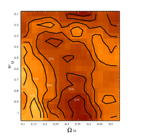
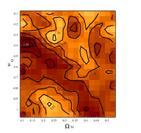
Which cosmologies are the most likely to produce significant features in $\xi(r)$ ? In order to answer this question we construct two significance maps which are shown in Fig. 2. The first map (upper panel) shows the percentage of scales in the $\xi(r)$ that shows $S/N\geq 1$ (significant features) averaged over the two redshift bins, while the second one (lower panel) shows the averaged $S/N$ for the $\xi(r)$ for two redshift bins, also using significant features only. The $\xi(r)$s are restricted to the range $100h^{-1}{\rm{Mpc}}\leq r\leq 300h^{-1}{\rm{Mpc}}$. In both panels of Fig. 2 lighter colours indicate higher values. From the first map we observe that our restriction on $S/N$ implies that the useful range of scales on the $\xi(r)$, on average, runs from 23% to 33%. On the other hand, the second map shows that the averaged $S/N$ lies in the range 1.39 to 1.51. From the contour levels and colours in this Fig. we can observe that there are many regions in both maps that are prone to a significant range of scales that are useful and a relatively high average $S/N$. Beyond that, an important issue that should be noticed is that all cosmological pairs on the map have useful scales in the $\xi(r)$ and therefore all models are plausible in showing coincident features at different times.

To quantify the level of agreement among $\xi(r)$s, we use the cross correlation denoted by $CC_{[1,2]}^{(2z)}$, where we have added an upper-script, $(2z)$, denoting the current case. This statistic has the capability of enhancing features that occur at similar scales while erasing those that do not appear at the same distance. Moreover, since there is a sum over a wide range of comoving scales, several coincident signals for a particular cosmological pair produce higher values of $CC$ implying a better match between the $\xi(r)$s at different redshifts.

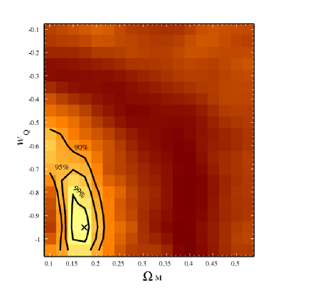
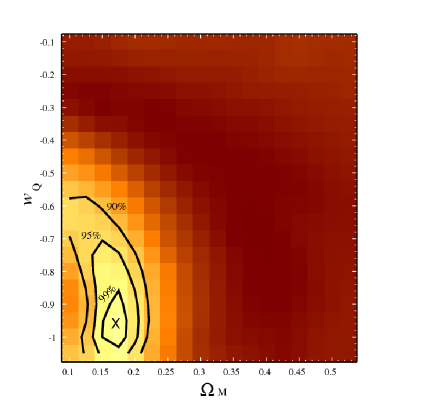
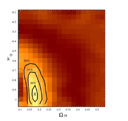
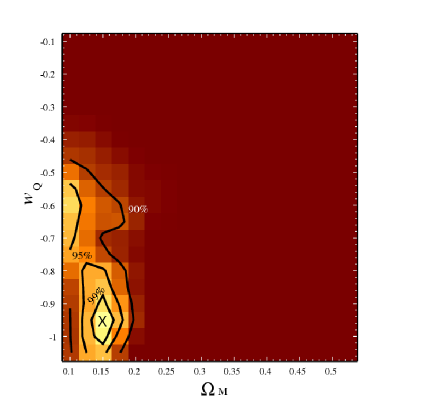
The $CC_{[1,2]}^{(2z)}$ maps with $r_{min}=110\ h^{-1}{\rm{Mpc}}$ are shown in Fig. 3. All panels show contour levels around the $CC_{[1,2]}^{(2z)}$ maxima that indicate the percentage of the map outside their boundaries. The upper left panel shows the $CC_{[1,2]}^{(2z)}$ computed taking into account all features (peaks and valleys) in the $\xi(r)$s. From this panel, we can see that the most likely cosmological models are in a small region in the lower left corner of the map. The black cross shows the maximum $CC_{[1,2]}^{(2z)}$ value that corresponds to $\Omega_{\rm M}=0.175$ and $w_{\rm Q}=-0.95$.

Since this result is achieved by using all features in the $\xi(r)$s, an interesting question is whether a particular feature (peaks or valleys) contributes to a particular region in the map. This issue can be answered by computing the cross correlation statistics using eq. 4, but taking into account positive (peaks) or negative (valleys) significant ($S/N\geq\ 1$) values of the $\xi(r)$ only. The resulting maps can be seen on the lower left (peaks only) and lower right (valleys only) panels in Fig. 3.

From the left panel, we can see that peaks restrict the area displayed by the contour levels compared with the ones obtained with all features. The contours are reduced, ruling out some cosmological pairs with $w_{\rm Q}\geq-0.6$ and are very slightly shifted to the right (higher values of $\Omega_{\rm M}$). Even so, the preferred cosmological pair remains unchanged. On the other hand, valleys alone give lower $\Omega_{\rm M}$ values ($\sim 0.150$) and produce an elongation of contour levels towards higher values of $w_{\rm Q}$. Nevertheless, their contribution to the combined feature analysis is not strong enough to prevail over the signal preferred by peaks.

Finally, it is interesting to know what would be the effect of relaxing the restriction imposed on the $S/N$ of the features. In the upper right panel of Fig. 3 we construct the $CC_{[1,2]}^{(2z)}$ map without imposing any value on the $S/N$ of the $\xi(r)$s. From the colour intensity of the map it is clear that the main effect (compared to the upper left panel) is the widening of the area of preferred cosmologies. Even when this map enhances the importance of some cosmological models that are not statistically significant, the resulting preferred cosmology turns out to be very similar to the one obtained from significant features only.

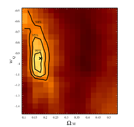
Since our result on $w_{\rm Q}$ is close to the limit of the $w_{\rm Q}$ range used so far, it would be interesting to test whether the exclusion of $w_{\rm Q}<-1.1$ is biasing our results. Therefore, we repeated the cross correlation analysis over a shifted range, $-1.45\leq w_{\rm Q}\leq-0.50$. As can be seen from Fig. 4 our results are stable, hence no bias arises from our original choice for the $w_{\rm Q}$ range.

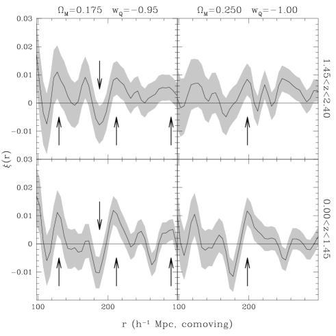
To illustrate the ability of our method to compare $\xi(r)$s at different times, in Fig. 5 we show a comparison between the best cosmological pair obtained using the $CC_{[1,2]}^{(2z)}$ map ($\Omega_{\rm M}=0.175$ and $w_{\rm Q}=-0.95$, left panels) and the standard model ($\Lambda CDM$, $\Omega_{\rm M}=0.250$ and $w_{\rm Q}=-1.00$, right panels). The grey region in each panel shows the $1\sigma$ bootstrap errors bars. The best model is clearly better than the standard one given the number of coincident significant features at different scales. The arrows in this Fig. show features observed at the same comoving scale that satisfy $S/N\geq\ 1$. While the preferred cosmological model obtained from our maps has four coincident features, we can only observe one matching feature for the standard cosmological model.

We have also checked whether the resulting best model depends on the choice of $r_{min}$ by computing $CC_{[1,2]}^{(2z)}$ maps varying $r_{min}$ from 120 to 190 $h^{-1}{\rm{Mpc}}$. In all cases we found that the preferred pair of cosmological parameters is the same obtained for $r_{min}=110\ h^{-1}{\rm{Mpc}}$, indicating the stability of our results.

3.2.3 The four redshift bin case

Given the size of the redshift bins used in the previous case, the evolution of the quasar population within each bin might be biasing the results. In this subsection, we use four redshift bins to avoid too much evolution within a single bin. This analysis tests the stability of the results obtained with two redshift bins even when narrower redshift bins imply larger errors in the $\xi(r)$. We divide the sample into four equal number redshift bins:

1. $0.00<z\leq 1.07$

2. $1.07<z\leq 1.45$

3. $1.45<z\leq 1.78$

4. $1.78<z\leq 2.40$.

With these subsamples we choose to calculate two estimates of the cosmological parameters using the cross correlations between redshift bins 1-3 and 2-4. This choice will give us two estimates statistically independent of each other, and, at the same time, by interleaving redshift bins, minimise evolutionary effects. This approach will also allow us to estimate random errors in the resulting cosmological parameters by computing the standard error in the mean between the two estimates. The resulting standard error can also be used as a fair estimate of random errors in the two redshift bin case.

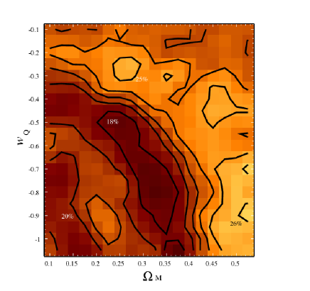
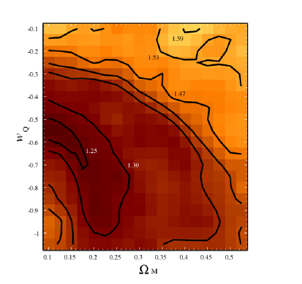
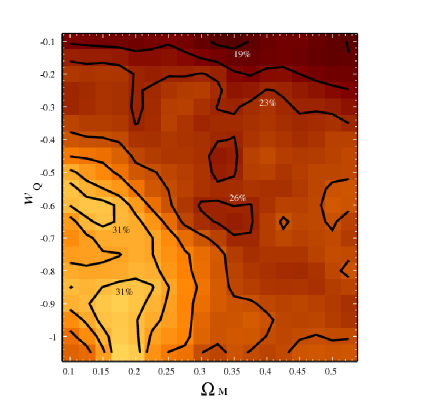
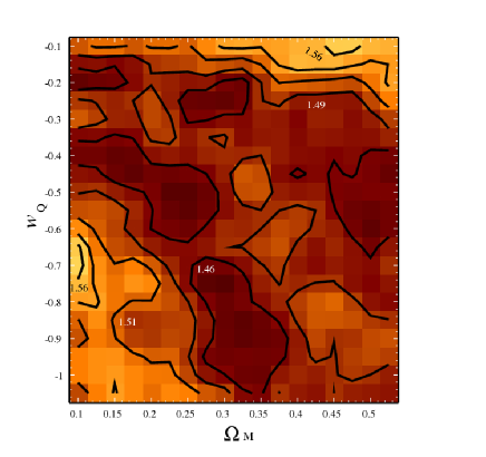
After computing the functions $\xi(r)$, we show in Fig. 6 the significance maps for the redshift bins 1-3 (upper panels) and 2-4 (lower panels). The percentage maps (left column) are shown for significant features averaged over two redshift bins. When combining redshift bins 1-3 (upper panel) we observe that 18%-26% is the range of scales for the $\xi(r)$’s that are useful for our study while 19%-31% is the range of scales obtained for redshift bins 2-4 (lower panel). On the other hand, when analysing the averaged $S/N$ maps (right column) for significant features only, the redshift bins 1-3 (upper panel) show a variation from 1.25 to 1.59 while the average over redshifts 2-4 (lower panel) lies in the range 1.46 to 1.56. It is clear that all cosmological pairs have some portion of the $\xi(r)$ useful for our study.

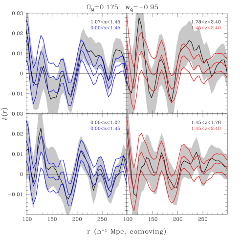
These $S/N$ maps span similar value ranges to those corresponding to the two redshift bin case (see Fig. 2). Even when computing the $\xi(r)$s within narrower redshift bins produces larger error bars, on average, the $S/N$ show no degradation compared to the previous case since some peaks and valleys in $\xi(r)$ are larger now. This could be a consequence of less evolution within a single redshift bin. Under this assumption, some features in the $\xi(r)$ in the two redshift bin case could have been eroded away by evolution. In Fig. 7 we observe a comparison between the $\xi(r)$s obtained in the two (blue and red curves) and four (grey areas) redshift bins cases for the preferred cosmological model found in the previous subsection. Examples of our statement are the regions with $200\ h^{-1}{\rm{Mpc}}\leq r\leq 250\ h^{-1}{\rm{Mpc}}$ in the two upper panels, and the peak at $\sim 130\ h^{-1}{\rm{Mpc}}$ in the lower left panel of this Fig.

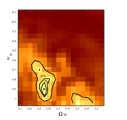
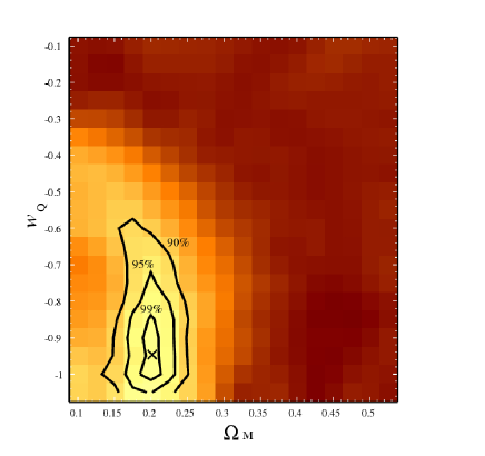
Figure 8 shows the cross correlation maps corresponding to the calculation of equation 4 for redshift bins 1-3 ($CC_{[1,3]}^{(4z)}$, left panel) and 2-4 ($CC_{[2,4]}^{(4z)}$, right panel). Each map is computed using $r_{min}=$ 110 $h^{-1}{\rm{Mpc}}$. The preferred model in the $CC_{[1,3]}^{(4z)}$ map is $\Omega_{\rm M}=0.225$ and $w_{\rm Q}=-0.90$. On the other hand, the $CC_{[2,4]}^{(4z)}$ map better fits with $\Omega_{\rm M}=0.200$ and $w_{\rm Q}=-0.95$. We have checked that these results do not change when varying $r_{min}$ from 120 to 190 $h^{-1}{\rm{Mpc}}$. From these results the mean cosmological values and their corresponding standard errors are $\Omega_{\rm M}=0.21\pm 0.02$ and $w_{\rm Q}=-0.93\pm 0.04$. We observe that this result is consistent within a $1\ \sigma$ interval with the one obtained for the two redshift bin case.

In the light of our results, we consider as the most likely cosmological model to be the one obtained for the four redshift bin case since it is less affected by evolution effects while having similar $S/N$ values to those obtained when using larger redshift bins.

Figure 7: Comparison of the $\xi(r)$s between the two (blue and red curves) and four (grey areas) redshift bin cases for the preferred model obtained in the two redshift bin case. Error bars were computed using the bootstrap re-sampling technique. Each panel quotes the corresponding redshift ranges.

Figure 8: ($\Omega_{\rm M}-w_{\rm Q}$) maps for the $CC^{(4z)}$ of the $\xi(r)$ for four redshift bins. The left panel show the $CC^{(4z)}_{[1,3]}$, while the right panels show $CC^{(4z)}_{[2,4]}$. The minimum comoving distance for each map is $r_{min}=$110 $h^{-1}{\rm{Mpc}}$. Each model is computed only for $S/N\geq$ 1. Higher values of the cross-correlation correspond to lighter colours. Labels in contour level show the percentage of the map outside the contours.

4 Summary and discussion

In this work we have studied the evolution of the quasar two-point correlation function, $\xi(r)$, to constrain cosmological parameters for flat quintessential universes, namely the matter adimensional density parameter $\Omega_{\rm M}$ and the quintessence equation of state, $w_{\rm Q}$. For this purpose, we have drawn a large homogeneous quasar sample from the SDSS DR6, the largest quasar catalogue available at present. The size and homogeneity of the sample allow for highly reliable statistical studies of quasars. As in previous studies of this aspect (e.g. Vallinotto et al. 2007; Sánchez et al. 2008; Crocce & Scoccimarro 2008), we have focused on analysing the position of features in $\xi(r)$, at large comoving scales ($r>100h^{-1}{\rm{Mpc}}$) well into the linear regime of structure formation. The key point of the analysis lies in the assumption that, for the proper cosmological model, the comoving length scale of such features in $\xi(r)$ should remain fixed at different stages in the evolution of the universe. In this work, we do not assume any particular scale at which the features (peaks and valleys) should be found, but we only require consistency among different redshifts ranges, imposing purely geometric constraints on the cosmological parameters.

The study is focused on two different complementary approaches: splitting the quasar redshift distribution into two and four redshifts bins. The first analysis is performed in order to have reliable estimations of $\xi(r)$ at large scales (where the signal is expected to be low) while the second one is performed aiming to rule out a possible bias in the previous results due to an evolution of the quasar population within a particular redshift bin. The comparison among $\xi(r)$s of different redshift bins is carried out by means of the cross-correlation function ($CC$). This particular statistic has the advantage of quantifying the amount of overlap between two functions. In our case, the $CC$s are computed for modified $\xi(r)$s, i.e, we have imposed a significance criterion which keeps the $\xi(r)$s values when they satisfy the constraint $|\xi(r)/\sigma(r)|\ \geq\ 1$, otherwise are set to zero.

With regard to the two redshift bin case, the most likely model is $\Omega_{\rm M}=0.18\pm 0.02$ and $w_{\rm Q}=-0.95\pm 0.04$. The coincidence among the results for the different reference scales ($r_{min}$) analysed is remarkable, implying that $\xi(r)$s for both redshift bins agree over a wide range of comoving scales, from $\sim 100$ to $\sim 300h^{-1}{\rm{Mpc}}$. From the four redshift bin case we obtain that the preferred cosmological model is $\Omega_{\rm M}=0.21\pm 0.02$ and $w_{\rm Q}=-0.93\pm 0.04$. When analysing the four redshift bin case, it becomes clear that the two redshift bin analysis is affected by evolution. The main observable effect of evolution is that, on average, the amplitude of some features in the $\xi(r)$ has been diminished, and as a consequence, the best model has been slightly shifted towards lower values of $\Omega_{\rm M}$.

The closest reference in the literature of an analysis similar to that performed in this work is the study of $R02$. Some of the similarities with this work are: we both only use a sample of quasars to constrain cosmological parameters, and neither of us search for a particular comoving scale. Beyond quasar sample sizes, the methodology differences can be enumerated as follows:

• We extract information from the position of peaks and valleys in the $\xi(r)$s while $R02$ used peak information only.

• We restrict the $\xi(r)$s with a significance criterion in order to avoid spurious detections while $R02$ used all the information without any restriction on $S/N$ ratio.

• The statistical tool proposed in this work intends to perform a full scale comparison among $\xi(r)$s, i.e, to take into account more than one feature agreement among different redshift bins. On the other hand, $R02$ developed a method based on searching for the largest probability that the first local maximum in $\xi(r)$ above a given reference scale occurs at the same comoving distance for consecutive redshift bins.

• By construction, our method gives larger weights to stronger features while the probability method of $R02$ only considers the comoving length scale at which a peak is present.

• We performed an analysis involving two and four redshift bins and found that evolution cannot be neglected. $R02$ performed their analysis using three redshift bins, extracting information from consecutive redshift bins. Their approach can still be affected by evolution effects.

In their work, $R02$ found a matter density parameter in good agreement with our findings (see Table 1). Nevertheless, they cannot impose strong constraints on the quintessence parameter, finding only an upper limit ($w_{\rm Q}\leq-0.50$). Therefore, our results show that using the full large scale shape of the $\xi(r)$s provides tighter constraints on cosmological parameters rather than basing the analysis on the coincidence of a single particular scale only.

Table 1: Constraints on cosmological parameters $\Omega_{\rm M}$ and $w_{\rm Q}$ found in the literature under the assumption of perfectly flat universes. The last column quotes the data sets used in each work.

Author	$\Omega_{\rm M}$	$w_{\rm Q}$	Data
Roukema et al. (2002)	$0.25\pm 0.10$	$[-1.0,-0.5]$	10K 2dFQSO1
Tegmark et al. (2004)	$0.329\pm 0.074$	$-0.92\pm 0.30$	WMAP2 + SDSS MGS3
Eisenstein et al. (2005)	$0.326\pm 0.037$	$-0.80\pm 0.18$	WMAP + SDSS MGS + LRG4
Wang & Mukherjee (2006)	…	$-0.885^{+0.109\leavevmode\nobreak\ +0.206}_{-0.111\leavevmode\nobreak\ -0.227}$	R045 WMAP36 + SNIa + LRG
Wang & Mukherjee (2006)	…	$-0.999^{+0.082\leavevmode\nobreak\ +0.159}_{-0.083\leavevmode\nobreak\ -0.168}$	A067 WMAP3 + SNIa + LRG
Sánchez et al. (2006)	$0.241\pm 0.024$	$-0.85^{+0.18}_{-0.17}$	WMAP + 2dFGRS8
Spergel et al. (2007)	$0.238\pm 0.015$	$-0.967\pm 0.073$	WMAP3 + SNLS9
This work	$0.21\pm 0.02$	$-0.93\pm 0.04$	DR6 SDSS QSO

1: Quasars from the 10K release of the 2 degree Field Quasar Redshift Survey, Croom et al. (2001).
2: First year Wilkinson Microwave Anisotropy Probe, Spergel et al. (2003).
3: Main Galaxy Sample, Strauss et al. (2002).
4: Luminous Red Galaxies, Eisenstein et al. (2001).
5: Riess et al. (2004).
6: Third year Wilkinson Microwave Anisotropy Probe, Spergel et al. (2007).
7: Astier et al. (2006).
8: 2 degree Field Galaxy Redshift Survey, Colless et al. (2001).
9: Supernovae Legacy Survey, Astier et al. (2006).

From the comparison with results from a variety of data and techniques (see Table 1), we observe that our estimation of $\Omega_{\rm M}$ is in good agreement with $R02$, Sánchez et al. (2006) and Spergel et al. (2007). In addition, our result for $w_{\rm Q}$ agrees with all sources quoted in Table 1, and has one of the smallest uncertainty intervals.

What are the possible implications of our results in terms of structure formation compared to the initial conditions established by the $\Lambda CDM$ concordance model? We observe a small discrepancy in the mean values obtained for the $\Omega_{\rm M}$ and $w_{\rm Q}$ compared with a standard universe with cosmological constant ($\Omega_{\rm M}=0.25$ and $w_{\rm Q}=-1.0$). Our results are prone to prefer cosmologies with slightly lower values of $\Omega_{\rm M}$ and higher values of $w_{\rm Q}$ than those of the concordance model. Both tendencies observed in the parameters have similar consequences for structure formation. If all cosmological models were normalised to predict the observed amplitude of density fluctuations at present, lower values of density would predict higher levels of density fluctuations in the past (e.g. Spergel 1998). Under the same assumptions of density perturbation normalisation, earlier cloud formation and higher core densities are observed if the dynamics of the dark energy is enhanced, i.e. for models represented by an equation of state parameter $w_{\rm Q}>-1$ (Bartelmann et al. 2002; Dolag et al. 2004; Maio et al. 2006). Hence, at a given mass and redshift our results would predict higher abundance of more concentrated halos than in the model with the cosmological constant.

Our results rely on the analysis of quasar clustering alone, demonstrating that it is plausible to put strong constraints on cosmological parameters with only one suitable data set and a proper statistical treatment. Since our results are independent of the cosmic microwave background, type Ia supernovae and galaxy data, then large quasar samples in combination with all these data sets should imply a better determination of $\Omega_{\rm M}$ and $w_{\rm Q}$.

References

- Adelman-McCarthy et al. (2008) Adelman-McCarthy, J. K., et al. 2008, ApJS, 175, 297
- Astier et al. (2006) Astier, P., et al. 2006, A&A, 447, 31
- Bartelmann et al. (2002) Bartelmann, M., Perrotta, F., & Baccigalupi, C. 2002, A&A, 396, 21
- Blanton et al. (2003) Blanton, M. R., Lin, H., Lupton, R. H., Maley, F. M., Young, N., Zehavi, I., & Loveday, J. 2003, AJ, 125, 2276
- Caldwell et al. (1998) Caldwell, R. R., Dave, R., & Steinhardt, P. J. 1998, Physical Review Letters, 80, 1582
- Chen & Ratra (2004) Chen, G., & Ratra, B. 2004, ApJ, 612, L1
- Colless et al. (2001) Colless, M., et al. 2001, MNRAS, 328, 1039
- Crocce & Scoccimarro (2008) Crocce, M., & Scoccimarro, R. 2008, Phys. Rev. D, 77, 023533
- Croom et al. (2001) Croom, S. M., Smith, R. J., Boyle, B. J., Shanks, T., Loaring, N. S., Miller, L., & Lewis, I. J. 2001, MNRAS, 322, L29
- Daly et al. (2007) Daly, R. A., Mory, M. P., O’Dea, C. P., Kharb, P., Baum, S., Guerra, E. J., & Djorgovski, S. G. 2007, ArXiv e-prints, 710, arXiv:0710.5112
- Dolag et al. (2004) Dolag, K., Bartelmann, M., Perrotta, F., Baccigalupi, C., Moscardini, L., Meneghetti, M., & Tormen, G. 2004, A&A, 416, 853
- Doré et al. (2007) Doré, O., et al. 2007, ArXiv e-prints, 712, arXiv:0712.1599
- Eisenstein et al. (2001) Eisenstein, D. J., et al. 2001, AJ, 122, 2267
- Eisenstein et al. (2005) Eisenstein, D. J., et al. 2005, ApJ, 633, 560
- Gong et al. (2008) Gong, Y., Wu, Q., & Wang, A. 2008, ApJ, 681, 27.
- Górski et al. (2005) Górski, K. M., Hivon, E., Banday, A. J., Wandelt, B. D., Hansen, F. K., Reinecke, M., & Bartelmann, M. 2005, ApJ, 622, 759
- Gunn et al. (1998) Gunn, J. E., et al. 1998, AJ, 116, 3040
- Guzik et al. (2007) Guzik, J., Bernstein, G., & Smith, R. E. 2007, MNRAS, 375, 1329
- Landy & Szalay (1993) Landy, S. D., & Szalay, A. S. 1993, ApJ, 412, 64
- La Vacca & Colombo (2008) La Vacca, G., & Colombo, L. P. L. 2008, Journal of Cosmology and Astro-Particle Physics, 4, 7
- Lima et al. (2007) Lima, J. A. S., Jesus, J. F., & Cunha, J. V. 2007, ArXiv e-prints, 709, arXiv:0709.2195
- Maio et al. (2006) Maio, U., Dolag, K., Meneghetti, M., Moscardini, L., Yoshida, N., Baccigalupi, C., Bartelmann, M., & Perrotta, F. 2006, MNRAS, 373, 869
- Mo et al. (1992) Mo, H. J., Jing, Y. P., & Borner, G. 1992, ApJ, 392, 452.
- Peebles (1984) Peebles, P. J. E. 1984, ApJ, 284, 439
- Perlmutter et al. (1999) Perlmutter, S., et al. 1999, ApJ, 517, 565
- Ratra & Peebles (1988) Ratra, B., & Peebles, P. J. E. 1988, Phys. Rev. D, 37, 3406
- Richards et al. (2002) Richards, G. T., et al. 2002, AJ, 123, 2945
- Riess et al. (1998) Riess, A. G., et al. 1998, AJ, 116, 1009
- Riess et al. (2004) Riess, A. G., et al. 2004, ApJ, 607, 665
- Roukema (2001) Roukema, B. F. 2001, A&A, 369, 729
- Roukema et al. (2002) Roukema, B. F., Mamon, G. A., & Bajtlik, S. 2002, A&A, 382, 397
- Sánchez et al. (2006) Sánchez, A. G., Baugh, C. M., Percival, W. J., Peacock, J. A., Padilla, N. D., Cole, S., Frenk, C. S., & Norberg, P. 2006, MNRAS, 366, 189
- Sánchez et al. (2008) Sánchez, A. G., Baugh, C. M., & Angulo, R. 2008, ArXiv e-prints, 804, arXiv:0804.0233
- Sapone & Amendola (2007) Sapone, D., & Amendola, L. 2007, ArXiv e-prints, 709, arXiv:0709.2792
- Santos & Lima (2008) Santos, R. C., & Lima, J. A. S. 2008, Phys. Rev. D, 77, 083505
- Schlegel et al. (1998) Schlegel, D. J., Finkbeiner, D. P., & Davis, M. 1998, ApJ, 500, 525
- Schneider et al. (2005) Schneider, D. P., et al. 2005, AJ, 130, 367
- Sen (2008) Sen, A. A. 2008, Phys. Rev. D, 77, 043508
- Shanks & Boyle (1994) Shanks, T., & Boyle, B. J. 1994, MNRAS, 271, 753.
- Spergel (1998) Spergel, D. N. 1998, Classical and Quantum Gravity, 15, 2589
- Spergel et al. (2003) Spergel, D. N., et al. 2003, ApJS, 148, 175
- Spergel et al. (2007) Spergel, D. N., et al. 2007, ApJS, 170, 377
- Strauss et al. (2002) Strauss, M. A., et al. 2002, AJ, 124, 1810
- Szydłowski et al. (2008) Szydłowski, M., Hrycyna, O., & Kurek, A. 2008, Phys. Rev. D, 77, 027302
- Tegmark et al. (2004) Tegmark, M., et al. 2004, Phys. Rev. D, 69, 103501
- Vallinotto et al. (2007) Vallinotto, A., Dodelson, S., Schimd, C., & Uzan, J.-P. 2007, Phys. Rev. D, 75, 103509
- Wang & Mukherjee (2006) Wang, Y., & Mukherjee, P. 2006, ApJ, 650, 1
- Wang & Mukherjee (2007) Wang, Y., & Mukherjee, P. 2007, Phys. Rev. D, 76, 103533
- Wei & Zhang (2008) Wei, H., & Zhang, S. N. 2008, ArXiv e-prints, 803, arXiv:0803.3292
- Yahata et al. (2005) Yahata, K., et al. 2005, PASJ, 57, 529
- York et al. (2000) York, D. G., et al. 2000, AJ, 120, 1579
- Zhang et al. (2007) Zhang, Q.-J., Cheng, L.-M., & Wu, Y.-L. 2007, ArXiv e-prints, 708, arXiv:0708.2164
- Zhu & Sereno (2008) Zhu, Z.-H., & Sereno, M. 2008, ArXiv e-prints, 804, arXiv:0804.2917