Regularity of multifractal spectra of conformal iterated function systems

Abstract.

We investigate multifractal regularity for infinite conformal iterated function systems (cIFS). That is we determine to what extent the multifractal spectrum depends continuously on the cIFS and its thermodynamic potential. For this we introduce the notion of regular convergence for families of cIFS not necessarily sharing the same index set, which guarantees the convergence of the multifractal spectra on the interior of their domain. In particular, we obtain an Exhausting Principle for infinite cIFS allowing us to carry over results for finite to infinite systems, and in this way to establish a multifractal analysis without the usual regularity conditions. Finally, we discuss the connections to the $\lambda$-topology introduced by Roy and Urbański.

1. Introduction and statement of results

The theory of multifractals has its origin at the boarderline between statistical physics and mathematics - classical references are e. g. [FP85, Man74, Man88, HJK⁺86]. In this paper we study multifractal spectra in the setting of infinite conformal iterated functions systems (cIFS). These systems are given by at most countable families $\Phi=\left(\varphi_{e}:X\to X\right)_{e\in I}$ , $I\subset\mathbb{N}$, of conformal contractions on a compact connected subset $X$ of the euclidean space $\left(\mathbb{R}^{D},\|\cdot\|\right)$, $D\geq 1$. The set of cIFS with fixed phase space $X$ will be denoted by $\mathrm{CIFS}\left(X\right)$ (see Section 2 for definitions). For $\omega\in I^{\mathbb{N}}$ we let $\omega_{|k}:=\omega_{1}\cdots\omega_{k}$ and $\varphi_{\omega_{|k}}:=\varphi_{\omega_{1}}\circ\cdots\circ\varphi_{\omega_{k}}$. Then for each $\omega\in I^{\mathbb{N}}$ the intersection $\bigcap_{k=1}^{\infty}\varphi_{\omega_{|k}}\left(X\right)$ is always a singleton given rise to a canonical coding map $\pi_{\Phi}:I^{\mathbb{N}}\to X$. Its image $\Lambda_{\Phi}:=\pi_{\Phi}\left(I^{\mathbb{N}}\right)$ will be called the limit set of $\Phi$. Given a Hölder continuous function $\psi:I^{\mathbb{N}}\longrightarrow\mathbb{R}$ the multifractal analysis of the system $\Phi$ with respect to the potential $\psi$ is in our context understood to be the analysis of the level sets

$$\mathcal{F}_{\alpha}:=\pi_{\Phi}\left\{\omega\in I^{\mathbb{N}}:\lim_{k\rightarrow\infty}\frac{S_{k}\psi\left(\omega\right)}{\log\bigl{\|}\varphi_{\omega_{|k}}^{\prime}\bigr{\|}_{X}}=\alpha\right\}$$

in terms of their Hausdorff dimension $f\left(\alpha\right):=\dim_{H}\left(\mathcal{F}_{\alpha}\right)$. In here, $S_{k}\psi:=\sum_{n=0}^{k-1}\psi\circ\sigma^{n}$ denotes the Birkhoff sum of $\psi$ with respect to the shift map $\sigma:I^{\mathbb{N}}\to I^{\mathbb{N}}$ on the symbolic space, and $\bigl{\|}\varphi_{\omega_{|k}}^{\prime}\bigr{\|}_{X}:=\sup_{x\in X}\bigl{|}\varphi_{\omega_{|k}}^{\prime}\left(x\right)\bigr{|}$ with $\bigl{|}\varphi_{\omega_{|k}}^{\prime}\left(x\right)\bigr{|}$ denoting the operator norm of the derivative. A good reference for this kind of multifractal analysis is provided e. g. in [Pes97].

Let us define the geometric potential function associated with $\Phi$ by $\zeta:I^{\mathbb{N}}\rightarrow\mathbb{R}_{0}^{-}$, $\zeta\left(\omega\right):=\log\left|\varphi^{\prime}_{\omega_{1}}\left(\pi\left(\sigma\left(\omega\right)\right)\right)\right|$. It is well known that in the case of finite cIFS, that is $\operatorname*{card}\left(I\right)<\infty$, $f$ can be related to the Legendre transform of the free energy function $t:\mathbb{R}\to\mathbb{R}$, which is defined implicitly by the pressure equation (cf. Definition 2.4)

$$\mathcal{P}\left(t\left(\beta\right)\zeta+\beta\psi\right)=0,\quad\beta\in\mathbb{R}.$$ (1.1)

More precisely, there exists a closed finite interval $J\subset\mathbb{R}$ such that for all $\alpha\in J$ we have

$$f\left(\alpha\right)=-t^{*}\left(-\alpha\right):=-\sup_{\beta}\left\{-\beta\alpha-t\left(\beta\right)\right\}=\inf_{\beta}\left\{t\left(\beta\right)+\beta\alpha\right\},$$ (1.2)

and for $\alpha\notin J$ we have $\mathcal{F}_{\alpha}=\varnothing$ ([Pes97, Theorem 21.1], [Sch99]). If we consider infinite cIFS, i. e. $\operatorname*{card}\left(I\right)=\operatorname*{card}\left(\mathbb{N}\right)$, we have to take into account that the pressure function might behave irregularly and hence it is not always possible to find a solution of (1.1). For the special case in which (1.1) has a unique solution the multifractal analysis has been discussed in [MU03, Section 4.9]. Further interesting results on the spectrum of local dimension for Gibbs states can be found [RU09].

Our first task is to generalise this concept to the case when the free energy cannot be defined by the unique solution of (1.1). This leads to the following modified definition of the free energy function.

Definition 1.1.

Let $\Phi\in\mathrm{CIFS}\left(X\right)$ and $\psi:I^{\mathbb{N}}\longrightarrow\mathbb{R}$ be a potential function. Then the free energy function $t:\mathbb{R}\longrightarrow\mathbb{R}\cup\left\{\infty\right\}$ for the pair $\left(\Phi,\psi\right)$ is given by

$$t\left(\beta\right):=\inf\left\{t\in\mathbb{R}:\mathcal{P}\left(t\zeta+\beta\psi\right)\leq 0\right\}.$$ (1.3)

Notice that our definition of the free energy function generalises the definition given for the multifractal analysis presented in [MU03, Section 4.9] or in [KU07], where the existence of a zero of the pressure function $t\longmapsto\mathcal{P}(t\zeta+\beta\psi)$ is always required. Our definition is rather in the spirit of [MU03, Theorem 4.2.13], which gives a version of Bowen’s formula, without assuming a zero of the pressure function to exist. More precisely, we have

$$\dim_{H}\left(\Lambda_{\Phi}\right)=\inf\left\{t\in\mathbb{R}:\mathcal{P}\left(t\zeta\right)\leq 0\right\},$$

which immediately implies that $t\left(0\right)=\dim_{H}\left(\Lambda_{\Phi}\right)$. In fact, Lemma 3.1 shows that Definition 1.1 gives rise to a proper convex function. This concept of the free energy function has been investigated further in [JKL10] as a special case of the induced topological pressure for arbitrary countable Markov shifts. We would like to point out that this new formalism gives rise to further interesting exhausting principles similar to Example 1.6 and Corollary 1.9 above.

To state our first main result we set

$$\alpha_{-}:=\inf\left\{-t^{-}\left(x\right):x\in\operatorname*{Int}\left(\operatorname*{dom}\left(t\right)\right)\right\}\;\mbox{and }\;\alpha_{+}:=\sup\left\{-t^{+}\left(x\right):x\in\operatorname*{Int}\left(\operatorname*{dom}\left(t\right)\right)\right\},$$

where $t^{+}$, resp. $t^{-}$, denotes the derivative of $t$ from the right, resp. from the left, $\operatorname*{Int}\left(A\right)$ denotes the interior of the set $A$, and $\operatorname*{dom}\left(t\right):=\left\{x\in\mathbb{R}:t\left(x\right)<+\infty\right\}$ refers to the effective domain of $t$.

Theorem 1.2.

For $\alpha\in\mathbb{R}$ we have $f\left(\alpha\right)\leq\max\left\{-t^{*}\left(-\alpha\right),0\right\}$ and for $\alpha\in\left(\alpha_{-},\alpha_{+}\right)$ we have $f\left(\alpha\right)=-t^{*}\left(-\alpha\right)$.

This first main result is essentially a consequence of the multifractal regularity property of sequences of tuples $\left(\Phi^{n},\psi^{n}\right)_{n}$ of iterated function systems and potentials, which is the second main concern of this paper.

We adapt the definition of pointwise convergence in $\mathrm{CIFS}\left(X\right)$ as used by Roy and Urbański in [RU05] to our setting, allowing us to investigate also families of cIFS with associated potentials not sharing the same index set $\mathbb{N}$. To simplify notation let us write $\|h\|_{\Omega}:=\sup_{\omega\in\Omega}\left|h\left(\omega\right)\right|$ for the supremum norm of the map $h:\Omega\longrightarrow\left(V,|\cdot|\right)$ from $\Omega$ to the normed space $\left(V,|\cdot|\right)$. For $\Phi^{1},\Phi^{2}\in\mathrm{CIFS}\left(X\right)$ we define

$$\rho\left(\Phi^{1},\Phi^{2}\right):=\sum_{i\in I_{1}\cap I_{2}}2^{-i}\left(\bigl{\|}\varphi_{i}^{1}-\varphi_{i}^{2}\bigr{\|}_{X}+\bigl{\|}(\varphi_{i}^{1})^{\prime}-(\varphi_{i}^{2})^{\prime}\bigr{\|}_{X}\right)+\sum_{i\in I_{1}\triangle I_{2}}2^{-i},$$ (1.4)

where $A\triangle B$ denotes the usual symmetric difference of the sets $A$ and $B$. It will turn out that $\rho$ defines a metric on $\mathrm{CIFS}\left(X\right)$. For $\omega\in\mathbb{N}^{k}$ and $k\in\mathbb{N}$ we let $\left[\omega\right]:=\left\{\tau\in\mathbb{N}^{\mathbb{N}}:\tau_{|k}=\omega\right\}$ denote the cylinder set of $\omega$.

In order to set up a multifractal spectrum we restrict our analysis to families of Hölder continuous functions $\psi^{n}:I_{n}^{\mathbb{N}}\longrightarrow\mathbb{R}$ and $\psi:I^{\mathbb{N}}\longrightarrow\mathbb{R}$ with $I_{n}\subset I\subset\mathbb{N}$, $n\in\mathbb{N}$.

Definition 1.3.

We say that $\left(\Phi^{n},\psi^{n}\right)_{n}\longrightarrow\left(\Phi,\psi\right)$ converges pointwise if,

1. $\Phi^{n}\longrightarrow\Phi$ in the $\rho$-metric and

2. for all $k\in I$ we have  ${\displaystyle\lim_{n\to\infty}\bigl{\|}\psi^{n}-\psi\bigr{\|}_{\left[k\right]\cap I_{n}^{\mathbb{N}}}=0}$.

Notice, that the convergence in $\rho$-metric implies that $\bigl{\|}\psi^{n}-\psi\bigr{\|}_{\left[k\right]\cap I_{n}^{\mathbb{N}}}$ in (B) is well defined for all sufficiently large $n$. For a further discussion of the above defined property see also the remark succeeding Lemma 2.6.

As discussed in [RU05] pointwise convergence topology leads to discontinuities of the Hausdorff dimension of the limit sets. By introducing a weaker topology called the $\lambda$-topology in [RU05] the Hausdorff dimension of the limit set depends continuously on the system (see also [RSU09]). Convergence in $\lambda$-topology requires the additional condition (6.1) below. As a corollary we will also establish the continuity of the Hausdorff dimension under weaker assumptions.

We are going to employ similar assumptions on the convergence of the pairs $\left(\Phi^{n},\psi^{n}\right)_{n}$ and $\left(\Phi,\psi\right)$ to obtain continuity of the multifractal spectra. This is the purpose of the following definition. For this let $\zeta^{n}$ denote the geometric potential associated with $\Phi^{n}$.

Definition 1.4.

We say that$\left(\Phi^{n},\psi^{n}\right)_{n}$ converges regularly to $\left(\Phi,\psi\right)$, if $\left(\Phi^{n},\psi^{n}\right)_{n}\longrightarrow\left(\Phi,\psi\right)$ converges pointwise, and if for $t,\beta\in\mathbb{R}$ with $\mathcal{P}(t\zeta+\beta\psi)<\infty$ there exists $k\in\mathbb{N}$ and a constant $C>0$ such that for all $n\in\mathbb{N}$ and all $\omega\in\left(I_{n}\right)^{k}$ we have

$$\exp\sup_{\tau\in I_{n}^{\mathbb{N}}\cap\left[\omega\right]}\left(S_{k}\left(t\zeta^{n}+\beta\psi^{n}\right)\left(\tau\right)\right)\leq C\exp\sup_{\rho\in I^{\mathbb{N}}\cap\left[\omega\right]}\left(S_{k}\left(t\zeta+\beta\psi\right)\left(\rho\right)\right).$$

The assumption in Definition 1.4 is similar to the corresponding inequality in the definition of the $\lambda$-topology in [RU05] but depends additionally on the potentials $\psi^{n}$ and $\psi$. For particular cases we will show that the convergence $\Phi^{n}\longrightarrow\Phi$ in the $\lambda$-topology immediately implies the conditions in Definition 1.4. This is demonstrated in the following example providing an analysis of the (inverse) Lyapunov spectrum. This example is covered by Proposition 6.4 (2) stated in Section 6.

Example 1.5 (${\bm{\lambda}}$-topology).

Let $\Phi^{n}=\left(\varphi_{e}^{n}\right)_{e\in I_{n}}$, $\Phi=\left(\varphi_{e}\right)_{e\in\mathbb{N}}$ be elements of $\mathrm{CIFS}\left(X\right)$ with $\Phi^{n}\rightarrow\Phi$ converging in the $\lambda$-topology and let $\psi^{n}=\psi=1$. Then $\left(\Phi^{n},\psi^{n}\right)_{n}\longrightarrow\left(\Phi,\psi\right)$ converges regularly.

The second example – eventhough straightforward to verify – is not only interesting for itself but will be of systematic importance for the proof of Theorem 1.2. See also Remark 5.1 and Example 1.9 for further discussion of this example.

Example 1.6 (Exhausting Principle I).

Let $\Phi=\left(\varphi_{e}\right)_{e\in\mathbb{N}}$ be an element of $\mathrm{CIFS}\left(X\right)$ and $\psi:I^{\mathbb{N}}\longrightarrow\mathbb{R}$ be Hölder continuous. Define $I_{n}:=I\cap\left\{1,\dots n\right\}$, $n\in\mathbb{N}$ and let $\Phi^{n}=\left(\varphi_{e}\right)_{e\in I_{n}}$ and $\psi^{n}:=\psi\big{|}_{I_{n}^{\mathbb{N}}}$. Then $\left(\Phi^{n},\psi^{n}\right)_{n}\longrightarrow\left(\Phi,\psi\right)$ converges regularly.

If the multifractal regularity property is satisfied we are able to prove the regularity of the free energy functions.

Theorem 1.7.

If $\left(\Phi^{n},\psi^{n}\right)_{n}\longrightarrow\left(\Phi,\psi\right)$ converges regularly then $t_{n}$ converges pointwise to $t$ on $\mathbb{R}$.

To state our second main result on the regularity of the multifractal spectra let

$$\mathcal{F}_{\alpha}^{n}:=\pi_{\Phi^{n}}\left\{\omega\in I_{n}^{\mathbb{N}}:\lim_{k\rightarrow\infty}\frac{S_{k}\left(\psi^{n}\right)\left(\omega\right)}{\log\bigl{\|}(\varphi_{\omega_{|k}}^{n})^{\prime}\bigr{\|}_{X}}=\alpha\right\},\quad f_{n}\left(\alpha\right):=\dim_{H}\left(\mathcal{F}_{\alpha}^{n}\right),$$

and with $t_{n}$ denoting the free energy function of $\left(\Phi^{n},\psi^{n}\right)$ let

$$\alpha_{-}^{n}:=\inf\left\{-t_{n}^{-}\left(x\right):x\in\operatorname*{Int}\left(\operatorname*{dom}\left(t_{n}\right)\right)\right\}\;\mbox{and }\;\alpha_{+}^{n}:=\sup\left\{-t_{n}^{+}\left(x\right):x\in\operatorname*{Int}\left(\operatorname*{dom}\left(t_{n}\right)\right)\right\}.$$

Theorem 1.8.

Let $\Phi^{n}=\left(\varphi_{e}^{n}\right)_{e\in I_{n}}$, $\Phi=\left(\varphi_{e}\right)_{e\in I}$ be elements of $\mathrm{CIFS}\left(X\right)$ and $\psi^{n},\psi$ be Hölder potentials such that $\left(\Phi^{n},\psi^{n}\right)_{n}\longrightarrow\left(\Phi,\psi\right)$ converges regularly. Then for each $\alpha\in\left(\alpha_{-},\alpha_{+}\right)$ we have

• $\lim_{n\to\infty}-t_{n}^{*}\left(-\alpha\right)=f\left(\alpha\right)=-t^{*}\left(-\alpha\right)$,

• $f_{n}\left(\alpha\right)=-t_{n}^{*}\left(-\alpha\right)$, for all $n$ sufficiently large.

In particular, we have $\limsup_{n}\alpha_{-}^{n}\leq\alpha_{-}\leq\alpha_{+}\leq\liminf_{n}\alpha_{+}^{n}.$ If additionally $\sup\operatorname*{dom}\left(t\right)=+\infty$ then $\liminf_{n}\alpha_{-}^{n}\geq\alpha_{-}$, whereas, if $\inf\operatorname*{dom}\left(t\right)=-\infty$ then $\limsup_{n}\alpha_{+}^{n}\leq\alpha_{+}$.

Combining the above theorems with Example 1.6 we obtain the following application of our analysis.

Corollary 1.9 (Exhausting Principle II).

Let $\Phi=\left(\varphi_{e}\right)_{e\in\mathbb{N}}$ be an element of $\mathrm{CIFS}\left(X\right)$, $\psi:I^{\mathbb{N}}\longrightarrow\mathbb{R}$ be Hölder continuous, and $\Phi^{n}=\left(\varphi_{e}\right)_{e\in I_{n}}$ and $\psi^{n}:=\psi\big{|}_{I_{n}^{\mathbb{N}}}$ with $I_{n}:=I\cap\left\{1,\dots n\right\}$, $n\in\mathbb{N}$. Then for each $\alpha\in\left(\alpha_{-},\alpha_{+}\right)$ we have $\lim_{n}-t_{n}^{*}\left(-\alpha\right)=f\left(\alpha\right)=-t^{*}\left(-\alpha\right)$ and $f_{n}\left(\alpha\right)=-t_{n}^{*}\left(-\alpha\right)$, for all $n$ sufficiently large. For the boundary points of the spectrum we have the following.

1. If $\operatorname*{dom}\left(t\right)=\mathbb{R}$ then $\lim_{n\to\infty}\alpha_{\pm}^{n}=\alpha_{\pm}$,

2. if $\sup\operatorname*{dom}\left(t\right)<+\infty$ then $\limsup_{n}\alpha_{-}^{n}=-\infty$ and for all $\alpha<\alpha_{-}$ we have

   $$\limsup_{n\to\infty}-t_{n}^{*}\left(-\alpha\right)\leq f\left(\alpha\right),$$

3. if $\inf\operatorname*{dom}\left(t\right)>-\infty$ then $\liminf_{n}\alpha_{+}^{n}=+\infty$ and for all $\alpha>\alpha_{+}$ we have

   $$\limsup_{n\to\infty}-t_{n}^{*}\left(-\alpha\right)\leq f\left(\alpha\right).$$

In Example 1.13 below we demonstrate how the lower bound on $f$ stated in Corollary 1.9 (3) can be applied.

Note that by virtue of Proposition 6.4 we have on the one hand that the convergence $\Phi^{n}\longrightarrow\Phi$ in the $\lambda$-topology implies that $\left(\Phi^{n},0\right)_{n}\longrightarrow\left(\Phi,0\right)$ converges regularly. On the other hand we have $t_{n}\left(0\right)=\dim_{H}\left(\Lambda_{\Phi^{n}}\right)$. Hence, the following corollary is straightforward and may be viewed as a generalisation of the continuity results in [RSU09, RU05] for the Hausdorff dimension of the limit sets.

Corollary 1.10 (Continuity of Hausdorff dimension).

Let $\Phi^{n}=\left(\varphi_{e}^{n}\right)_{e\in I_{n}}$, $\Phi=\left(\varphi_{e}\right)_{e\in I}$ be elements of $\mathrm{CIFS}\left(X\right)$ such that $\left(\Phi^{n},0\right)_{n}\longrightarrow\left(\Phi,0\right)$ converges regularly. Then

$$\lim_{n\to\infty}\dim_{H}\left(\Lambda_{\Phi^{n}}\right)=\dim_{H}\left(\Lambda_{\Phi}\right).$$

Finite-to-infinite phase transition

To complete the discussion of the Exhausting Principle we would like to emphasise that the boundary values of the approximating spectra in general do not converge to the corresponding value of the limiting system, i. e. we may have

$$f_{n}\left(\alpha_{\pm}^{n}\right)\not\to f\left(\alpha_{\pm}\right).$$ (1.5)

We refer to the property of an infinite system having a discontinuity of this kind in one of the boundary points as a finite-to-infinite phase transition in $\alpha_{+}$, resp. $\alpha_{-}$. Let us illustrate this property with the following concrete example.

Example 1.11 (Gauss system).

Let $\Phi:=\left\{\varphi_{e}:x\mapsto 1/\left(x+e\right):e\in\mathbb{N}\right\}$ denote the Gauss system and the potential $\psi$ is given by $\psi\left(\omega\right):=-2\log\omega_{1}$, for $\omega\in\mathbb{N}^{\mathbb{N}}$. In [JK10] we have shown that the multifractal spectrum is unimodal, defined on $\left[0,1\right]$, and in the boundary points of the spectrum we have $f(0)=0$ and $f(1)=1/2$. Nevertheless, for the exhausting systems $\Phi^{n}:=\left(\varphi_{e}\right)_{1\leq e\leq n}$ and $\psi^{n}:=\psi\big{|}_{\left\{1,\ldots,n\right\}^{\mathbb{N}}}$ we have for their corresponding multifractal spectra $f_{n}\left(\alpha_{+}^{n}\right)=0$ for all $n\in\mathbb{N}$ giving rise to a finite-to-infinite phase transition (see Fig 1.1). A proof of this will be postponed to the end of Section 5.

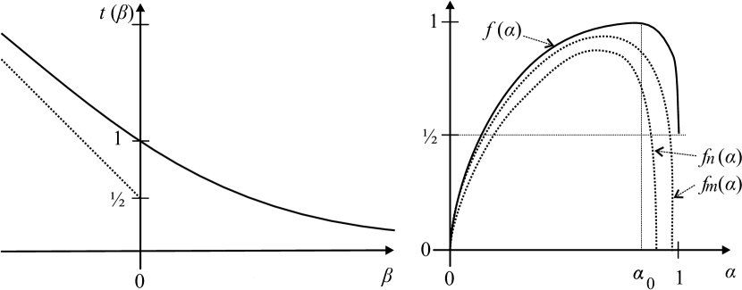
Figure 1.1. Sketch illustrating the finite-to-infinite phase transition for the Gauss system. The dashed graphs are associated to the approximating spectra $f_{n}:\left[0,\alpha_{+}^{n}\right]\to\mathbb{R}_{+}$ and $f_{m}:\left[0,\alpha_{+}^{m}\right]\to\mathbb{R}_{+}$, $m>n$, of finite sub-systems to the multifractal spectrum $f$ of the infinite system.

Example 1.12 (Lüroth system).

In the following example the effective domain of the free energy function is not equal to $\mathbb{R}$, which leads to an interesting boundary behaviour. For this let us consider the Lüroth system $\Phi:=\left\{\varphi_{n}:x\mapsto x/(n(n+1))+1/\left(n+1\right):n\in\mathbb{N}\right\}$ (essentially a linearised Gauss system) and the potential functions $\psi$ given by $\psi\left(\omega\right):=-\omega_{1}$, $\omega\in\mathbb{N}^{\mathbb{N}}$. Then in virtue of our theorems the spectrum is given by the Legendre transform of $t$ on $\left(2/\log\left(6\right),+\infty\right)$ via $f\left(\alpha\right)=-t^{*}\left(-\alpha\right)$. Similarly as for the Gauss system in the example above, one can show that $f\left(2/\log\left(6\right)\right)=f_{n}\left(2/\log\left(6\right)\right)=f_{n}\left(\alpha_{+}^{n}\right)=0$, $n\in\mathbb{N}$. Since we have Lebesgue almost everywhere that $\lim_{k\to\infty}\sum_{i=1}^{k}a_{i}/\sum_{i=1}^{k}\log\left(a_{i}\left(a_{i}+1\right)\right)=\int\left(\pi_{\Phi}^{-1}\left(x\right)\right)_{1}\,\mbox{d}\lambda/\int\log\left(\left(\pi_{\Phi}^{-1}\left(x\right)\right)_{1}\left(\left(\pi_{\Phi}^{-1}\left(x\right)\right)_{1}+1\right)\right)\,\mbox{d}\lambda=+\infty$ we find $f\left(+\infty\right)=1$. Hence as above, we have a finite-to-infinite phase transition – this time at infinity.

Example 1.13 (Generalised Lüroth system).

In the following example the effective domain of the free energy function is again not equal to $\mathbb{R}$ and additionally we have a second order phase transition. Let us consider the generalised Lüroth system $\Phi:=\left\{\varphi_{n}:x\mapsto 4x/\left(n(n+1)(n+2)\right)+2/\left(\left(n+1\right)\left(n+2\right)\right):n\in\mathbb{N}\right\}$ and the potential functions $\psi$ given by $\psi\left(\omega\right):=-\omega_{1}$, $\omega\in\mathbb{N}^{\mathbb{N}}$. Then in virtue of our theorems the spectrum is given by the Legendre transform of $t$ on $\left(3/\log\left(15\right),\alpha_{+}\right)$ via $f\left(\alpha\right)=-t^{*}\left(-\alpha\right)$, where $\alpha_{+}:=\left(2\sum_{n\geq 1}\frac{\log\left(\left(n(n+1)(n+2)\right)/4\right)}{\left(n(n+1)(n+2)\right)}\right)^{-1}$. Using the Corollary 1.9 (Exhausting Principle II) (3) we gather some extra information on the spectrum. Since we have $\lim_{n}-t_{n}^{*}\left(-t^{\prime}_{n}\left(0\right)\right)=1$ and $\alpha_{+}^{n}=n/\log(n(n+1)(n+2)/4)\to\infty$, we deduce that $1$ is a lower bound for $f\left(\alpha\right)$ for all $\alpha\geq\alpha_{+}$. Similarly as for the Gauss system in the example above, one can show that $f\left(3/\log\left(15\right)\right)=f_{n}\left(3/\log\left(15\right)\right)=f_{n}\left(\alpha_{+}^{n}\right)=0$, $n\in\mathbb{N}$. Hence, $f\left(\alpha\right)=-t^{*}\left(-\alpha\right)$ for all $\alpha\geq 3/\log(15)$. (cf. Fig. 1.2).

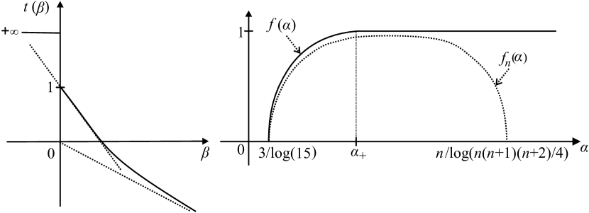
Figure 1.2. Sketch of the free energy function $t$ and the multifractal spectrum $f$ for the generalised Lüroth system. The dashed graph is associated to the approximating spectra $f_{n}:\left[3/\log\left(15\right),n/\log(n(n+1)(n+2)/4)\right]\to\mathbb{R}_{+}$ of finite sub-system to the multifractal spectrum $f$ of the infinite system.

Generalising further the latter two examples our analysis has successfully been applied in [KMS10] to determine the Lyapunov spectrum of $\alpha$-Farey-Lüroth and $\alpha$-Lüroth systems.

Example 1.14 (Irregular cIFS).

For this example we suppose that $\Phi$ is an irregular infinite cIFS, that is the range of the pressure function $p:t\mapsto\mathcal{P}\left(t\zeta\right)$ consists of the negative reals and infinity (see [MU03] for explicit examples), and let $\psi$ be constantly equal to $-1$. We suppose that $p\left(\delta\right)=\eta<0$, where $\delta$ is the critical value as well as the Hausdorff dimension of the limit set. Then the free energy function $t$ is given by $t\left(\beta\right)=p^{-1}\left(\beta\right)$ for $\beta<\eta$ and constantly equal to $\delta$ for $\beta\geq\eta$. The corresponding spectrum will have a linear part in $(0,\alpha_{-})$ if $-p^{+}\left(\delta\right)=1/\alpha_{-}<\infty$ and hence for $\alpha_{-}>0$, we observe a second order phase transition (see Fig. 1.3).

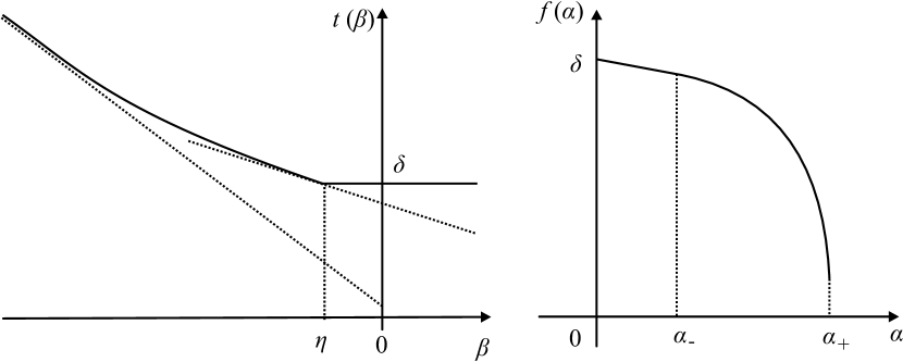
Figure 1.3. Sketch of the free energy function $t$ and the multifractal spectrum $f$ for an irregular system with constant negative potential. Note that in this situation we have a second order phase transition in $\alpha_{-}$ and the spectrum $f$ is linear on $(0,\alpha_{-})$.

The paper is organised as follows. In Section 2 we recall the basic notions relevant for cIFS. In Section 3 we show the regularity of the free energy function proving Theorem 1.7. Section 4 provides us with the necessary prerequisites from convex analysis allowing us to deduce the multifractal regularity in Section 5. In particular, we prove Theorem 1.2 and 1.8, and the finite-to-infinite phase transition for the Gauss system. The final section is devoted to the connection between our notion of regularity and the $\lambda$-topology.

2. Preliminaries

Let us recall the definition of a conformal iterated function system (see [MU03] for further details). Let $X$ be a compact metric space. For an alphabet $I\subset\mathbb{N}$ with $\operatorname*{card}\left(I\right)\geq 2$ we call $\Phi=\left(\varphi_{e}\right)_{e\in I}$ an iterated function system (IFS), where $\varphi_{e}:X\rightarrow X$ are injective contractions, $e\in I$, with Lipschitz constants globally bounded away from $1$.

Let $I^{*}:=\bigcup_{n\in\mathbb{N}}I^{n}$ denote the set of all finite subwords of $I^{\mathbb{N}}$. We will consider the left shift map $\sigma:I^{\mathbb{N}}\rightarrow I^{\mathbb{N}}$ defined by $\sigma\left(\omega_{i}\right):=\left(\omega_{i+1}\right)_{i\geq 1}$. For $\omega\in I^{*}$ we let $|\omega|$ denote the length of the word $\omega$, i. e. the unique $n\in\mathbb{N}$ such that $\omega\in I^{n}$.

The space $I^{\mathbb{N}}$ is equipped with the metric $d$ given by $d(\omega,\tau):=\exp\left(-|\omega\wedge\tau|\right),$ where $\omega\wedge\tau\in I^{*}\cup I^{\mathbb{N}}$ denotes the longest common initial block of the infinite words $\omega$ and $\tau$.

We now describe the limit set of the iterated function system $\Phi$. For each $\omega\in I^{*}$, say $\omega\in I^{n}$, we consider the map coded by $\omega$,

$$\varphi_{\omega}:=\varphi_{\omega_{1}}\circ\cdots\circ\varphi_{\omega_{n}}:X\rightarrow X.$$

For $\omega\in I^{\mathbb{N}}$, the sets $\left\{\varphi_{\omega|_{n}}\left(X\right)\right\}_{n\geq 1}$ form a descending sequence of non-empty compact sets and therefore $\bigcap_{n\geq 1}\varphi_{\omega|_{n}}\left(X\right)\neq\varnothing$. Since for every $n\in\mathbb{N}$, $\mathrm{diam}\left(\varphi_{\omega|_{n}}\left(X\right)\right)\leq s_{\Phi}^{n}\mathrm{diam}\left(X\right)$, we conclude that the intersection $\bigcap\varphi_{\omega|_{n}}\left(X\right)\in X$ is a singleton and we denote its only element by $\pi_{\Phi}(\omega)$. In this way we have defined the coding map $\pi=\pi_{\Phi}:I^{\mathbb{N}}\rightarrow X.$ The set $\Lambda=\Lambda_{\Phi}=\pi\left(I^{\mathbb{N}}\right)$ will be called the limit set of $\Phi$.

Definition 2.1.

We call an iterated function system conformal (cIFS) if the following conditions are satisfied.

1. The phase space $X$ is a compact connected subset of a Euclidean space $\mathbb{R}^{D}$, $D\geq 1$, such that $X$ is equal to the closure of its interior, i. e. $X=\overline{\operatorname*{Int}(X)}$.

2. (Open set condition (OSC)) For all $a,b\in I$, $a\neq b$,

   $$\varphi_{a}\left(\operatorname*{Int}(X)\right)\cap\varphi_{b}\left(\operatorname*{Int}(X)\right)=\varnothing.$$

3. There exists an open connected set $W\supset X$ such that for every $e\in I$ the map $\varphi_{e}$ extends to a $C^{1}$ conformal diffeomorphism of $W$ into $W$.

4. (Cone property) There exist $\gamma,l>0$, $\gamma<\pi/2$, such that for every $x\in X\subset\mathbb{R}^{D}$ there exists an open cone $\operatorname*{Con}(x,\gamma,l)\subset\operatorname*{Int}(X)$ with vertex $x$, central angle of measure $\gamma$, and altitude $l$.

5. There are two constants $L=L_{\Phi}\geq 1$ and $\alpha=\alpha_{\Phi}>0$ such that

   $$\left||\varphi_{e}^{\prime}(y)|-|\varphi_{e}^{\prime}(x)|\right|\leq\frac{L_{\Phi}}{\|(\varphi_{e}^{\prime})^{-1}\|_{X}}\|y-x\|^{\alpha}$$

   for every $e\in I$ and every pair of points $x,y\in X$.

For the following let

$$s_{\Phi}:=\sup_{e\in I}\left\|\left(\varphi_{e}\right)^{\prime}\right\|_{X}<1.$$ (2.1)

For a fixed phase space $X$ satisfying (a) the set of conformal iterated function systems will be denoted

$$\mathrm{CIFS}\left(X\right):=\left\{\Phi=\left(\varphi_{e}:X\longrightarrow X\right)_{e\in I}\textrm{ cIFS, }I\subset\mathbb{N}\right\}.$$

The following fact was proved in [MU03].

Proposition 2.2.

For $D\geq 2$, any family $\Phi=\left(\varphi_{e}\right)_{e\in I}$ satisfying condition (a) and (c) also satisfies condition (e) with $\alpha=1$.

In [MU03] we also find the following straightforward consequence of (e).

Lemma 2.3.

If $\Phi=\left(\varphi_{e}\right)_{e\in I}$ is a cIFS, then for all $\omega\in I^{*}$ and all $x,y\in W$, we have

$$\left|\log|\varphi_{\omega}^{\prime}(y)|-\log|\varphi_{\omega}^{\prime}(x)|\right|\leq\frac{L}{1-s^{\alpha}}\|y-x\|^{\alpha}.$$

Another consequence of (e) is

• (Bounded distortion property). There exists $K_{\Phi}\geq 1$ such that for all $\omega\in I^{*}$ and all $x,y\in X$

  $$|\varphi_{\omega}^{\prime}(y)|\leq K_{\Phi}|\varphi_{\omega}^{\prime}(x)|.$$

In [MU03, Lemma 2.3.1] it has been shown that for a Hölder continuous function $g:J^{\mathbb{N}}\rightarrow\mathbb{R}$, $J\subset I$, we have for all $\omega\in J^{*}$ and all $x,y\in\left[\omega\right]$ that

$$\exp S_{\left|\omega\right|}g\left(x\right)\leq K_{g}\exp S_{\left|\omega\right|}g\left(y\right).$$

In here, the constant $K_{g}\geq 1$ only depends on the Hölder norm and the Hölder exponent of $g$, as well as the metric on $J^{\mathbb{N}}$. With

$$Z_{n}\left(g\right):=\sum_{\omega\in J^{n}}\exp\sup_{\tau\in[\omega]\cap J^{\mathbb{N}}}\left(S_{n}g\left(\tau\right)\right)$$

we will denote the $n$-th partition function of $g$.

Definition 2.4.

The topological pressure $\mathcal{P}(f)$ of a continuous function $f:I^{\mathbb{N}}\rightarrow\mathbb{R}$ is defined by the following limit, which always exists (possibly equal to $+\infty$),

$$\mathcal{P}(f):=\lim_{n\rightarrow\infty}\frac{1}{n}\log Z_{n}\left(f\right)=\inf_{n}\frac{1}{n}\log Z_{n}\left(f\right).$$

At the end of this section we would like to comment on the topology of pointwise convergence. $\rho$ is well defined, since $\bigl{\|}\varphi_{i}^{1}-\varphi_{i}^{2}\bigr{\|}_{X}+\bigl{\|}(\varphi_{i}^{1})^{\prime}-(\varphi_{i}^{2})^{\prime}\bigr{\|}_{X}$ is bounded by $\mathrm{diam}\left(X\right)+2$. Using the fact that $A\triangle C\subset A\triangle B\cup B\triangle C$ for arbitrary sets $A,B,C$, we readily observe that $\rho$ as given in (1.4) actually defines a metric on $\mathrm{CIFS}\left(X\right)$. This metric induces the topology of pointwise convergence on $\mathrm{CIFS}\left(X\right)$. Let $\Phi^{n}=\left(\varphi_{i}^{n}:X\longrightarrow X\right)_{i\in I_{n}},$ $n\in\mathbb{N}$, and $\Phi=\left(\varphi_{i}:X\longrightarrow X\right)_{i\in I}$ be elements of $\mathrm{CIFS}\left(X\right)$ with $\Phi^{n}\rightarrow\Phi$ pointwise. Then for every $k\in\mathbb{N}$ we find an integer $N_{k}$ such that and all $n\geq N_{k}$ we have $I_{n}\triangle I\subset\left\{k+1,k+2,\dots\right\}.$ Similarly as in [RU05, Lemma 5.1] it follows that pointwise convergence in $\mathrm{CIFS}\left(X\right)$ is equivalent to the following condition.

Condition 2.5.

We have $\left(\Phi^{n},\psi^{n}\right)\rightarrow\left(\Phi,\psi\right)$ pointwise if and only if for every $\omega\in I^{*}$

$$\lim_{n\rightarrow\infty}\left(\bigl{\|}\varphi_{\omega}^{n}-\varphi_{\omega}\bigr{\|}_{X}+\bigl{\|}(\varphi_{\omega}^{n})^{\prime}-\varphi_{\omega}^{\prime}\bigr{\|}_{X}\right)=0\quad\mbox{and }\lim_{n\rightarrow\infty}\left(\bigl{\|}S_{|\omega|}\psi^{n}-S_{|\omega|}\psi\bigr{\|}_{\left[\omega\right]\cap I_{n}^{\mathbb{N}}}\right)=0$$

Using this condition we are able to prove a technical property which will be crucial in the proof of our main theorems.

Lemma 2.6.

Assume that $\left(\Phi^{n},\psi^{n}\right)\rightarrow\left(\Phi,\psi\right)$ converges pointwise. Then there exists $M>0$ such that for every $\omega\in I^{*}$ fixed and all sufficiently large $n\in\mathbb{N}$ (depending on $\omega$) we have for all $\eta\in\left[\omega\right]\cap I_{n}^{\mathbb{N}}$ and $\tau\in\left[\omega\right]\cap I^{\mathbb{N}}$

$$\frac{\mathrm{e}^{S_{|\omega|}\psi^{n}\left(\eta\right)}}{\mathrm{e}^{S_{|\omega|}\psi\left(\tau\right)}},\frac{\mathrm{e}^{S_{|\omega|}\zeta^{n}\left(\eta\right)}}{\mathrm{e}^{S_{|\omega|}\zeta\left(\tau\right)}}\in\left[M^{-1},M\right].$$

Proof.

Using the above Condition 2.5 we find for $\omega\in I^{*}$ and $n$ sufficiently large that

$$\max\left\{\bigl{\|}\log\left|\left(\varphi_{\omega}^{n}\right)^{\prime}\right|-\log\left|\left(\varphi_{\omega}\right)^{\prime}\right|\bigr{\|}_{X},\bigl{\|}S_{|\omega|}\psi^{n}-S_{|\omega|}\psi\bigr{\|}_{\left[\omega\right]\cap I_{n}^{\mathbb{N}}}\right\}\leq 1.$$

Then we have with $K_{\Phi}$ and $K_{\psi}$ denoting the bounded distortion constants as defined above

$$\left|S_{|\omega|}\zeta^{n}\left(\eta\right)-S_{|\omega|}\zeta\left(\tau\right)\right| =\left|\log\left|\left(\varphi_{\omega}^{n}\right)^{\prime}\right|\left(\pi_{\Phi^{n}}\left(\sigma^{n}\left(\eta\right)\right)\right)-\log\left|\left(\varphi_{\omega}\right)^{\prime}\right|\left(\pi_{\Phi}\left(\sigma^{n}\left(\tau\right)\right)\right)\right|$$

$$\leq\left|\log\left|\left(\varphi_{\omega}^{n}\right)^{\prime}\right|\left(\pi_{\Phi^{n}}\left(\sigma^{n}\left(\eta\right)\right)\right)-\log\left|\left(\varphi_{\omega}\right)^{\prime}\right|\left(\pi_{\Phi^{n}}\left(\sigma^{n}\left(\eta\right)\right)\right)\right|$$

$$\qquad+\left|\log\left|\left(\varphi_{\omega}\right)^{\prime}\right|\left(\pi_{\Phi^{n}}\left(\sigma^{n}\left(\eta\right)\right)\right)-\log\left|\left(\varphi_{\omega}\right)^{\prime}\right|\left(\pi_{\Phi}\left(\sigma^{n}\left(\tau\right)\right)\right)\right|$$

$$\leq 1+\log K_{\Phi}$$

as well as

$$\left|S_{|\omega|}\psi^{n}\left(\eta\right)-S_{|\omega|}\psi\left(\tau\right)\right| \leq\left|S_{|\omega|}\psi^{n}\left(\eta\right)-S_{|\omega|}\psi\left(\eta\right)\right|+\left|S_{|\omega|}\psi\left(\eta\right)-S_{|\omega|}\psi\left(\tau\right)\right|$$

$$\leq 1+\log K_{\psi}.$$

Letting $M:=3\cdot\max\left\{K_{\Phi},K_{\psi}\right\}$ the lemma follows. ∎

Remark 2.7.

Note that we may replace condition (B) in Definition 1.3 by the slightly weaker conditions on $\psi^{n}$ and $\psi$ stated in the above Lemma combined with the condition that $\psi^{n}$ converges uniformly to $\psi$ on compact $\sigma$-invariant subsets of $I^{\mathbb{N}}$.

3. Regularity of the free energy function

In this section we give a proof of Theorem 1.7. Let $\zeta$ denote the geometric potential function associated with $\Phi$ as defined in the introduction. For $\Phi\in\mathrm{CIFS}\left(X\right)$ and a Hölder continuous potential $\psi:I^{\mathbb{N}}\longrightarrow\mathbb{R}$ let $t$ denote the free energy function of $\left(\Phi,\psi\right)$ as introduced in Definition 1.1, i. e. $t\left(\beta\right):=\inf\left\{t:\mathcal{P}\left(t\zeta+\beta\psi\right)\leq 0\right\}$. Clearly, if there exists a zero of $t\longmapsto\mathcal{P}(t\zeta+\beta\psi)$ then $t\left(\beta\right)$ is the unique zero of this function (which in particular is the case for a finite alphabet $I$). Also, $t\left(\beta\right)=+\infty$ if and only if $\left\{t:\mathcal{P}\left(t\zeta+\beta\psi\right)\leq 0\right\}=\varnothing$.

Lemma 3.1.

The free energy $t$ of $\left(\Phi,\psi\right)$ is a proper (not necessarily closed) convex function on $\mathbb{R}$.

Proof.

Fix $\beta_{1},\beta_{2}\in\mathbb{R}$, $\lambda\in\left(0,1\right)$ and $\epsilon>0$. Using the convexity of the topological pressure we have

$$\mathcal{P}\left(\left(\lambda t\left(\beta_{1}\right)+\left(1-\lambda\right)t\left(\beta_{2}\right)+\epsilon\right)\zeta+\left(\lambda\beta_{1}+\left(1-\lambda\right)\beta_{2}\right)\psi\right)$$

$$\quad\quad=\mathcal{P}\left(\lambda\left(\left(t\left(\beta_{1}\right)+\epsilon\right)\zeta+\beta_{1}\psi\right)+\left(1-\lambda\right)\left(\left(t\left(\beta_{2}\right)+\epsilon\right)\zeta+\beta_{2}\psi\right)\right)$$

$$\quad\quad\leq\lambda\mathcal{P}\left(\left(t\left(\beta_{1}\right)+\epsilon\right)\zeta+\beta_{1}\psi\right)+\left(1-\lambda\right)\mathcal{P}\left(\left(t\left(\beta_{2}\right)+\epsilon\right)\zeta+\beta_{2}\psi\right)\leq 0.$$

Hence, by definition of $t$, this implies $t\left(\lambda\beta_{1}+\left(1-\lambda\right)\beta_{2}\right)\leq\lambda t\left(\beta_{1}\right)+\left(1-\lambda\right)t\left(\beta_{2}\right)+\epsilon$. Since $\epsilon>0$ was arbitrary this shows the convexity.

To see that $t$ is a proper convex function observe that $-\infty<\mathcal{P}\left(\beta\psi\right)$ and hence, for $t<0$, we have

$$\frac{1}{n}\log\sum_{\omega\in I^{n}}\exp\sup_{\tau\in\left[\omega\right]}\left(S_{n}t\zeta\left(\tau\right)+\beta\psi\right)\geq t\log\left(s_{\Phi}\right)+\mathcal{P}\left(\beta\psi\right)\to\infty\quad\mbox{ for }t\to-\infty.$$

Consequently, $t\left(\beta\right)>-\infty$ for all $\beta\in\mathbb{R}$. Since also $t\left(0\right)=\dim_{H}\left(\Lambda_{\Phi}\right)<\infty$ we have that $t$ is proper. ∎

Lemma 3.2.

Let $\left(\Phi^{n},\psi^{n}\right)_{n}\longrightarrow\left(\Phi,\psi\right)$ converge regularly. Then for all $t,\beta\in\mathbb{R}$ and $n$ tending to infinity we have

$$\mathcal{P}(t\zeta^{n}+\beta\psi^{n})\longrightarrow\mathcal{P}(t\zeta+\beta\psi).$$

Proof.

Fix $t,\beta\in\mathbb{R}$ with $\mathcal{P}(t\zeta+\beta\psi)<\infty$ and $\epsilon>0$. With $k\in\mathbb{N}$ and $C>0$ chosen according to Definition 1.4 choose $m\in\mathbb{N}$ large enough such that $\left(mk\right)^{-1}\log Z_{mk}\left(t\zeta+\beta\psi\right)\leq\mathcal{P}\left(t\zeta+\beta\psi\right)+\epsilon/2$ and $\left(mk\right)^{-1}\log\left(K+1\right)<\epsilon/2$, where $K:=M^{\left|\beta\right|+|t|}$ and $M$ is the constant defined in the proof of Lemma 2.6. We prove that for all $n\in\mathbb{N}$ sufficiently large we have

$$\left(mk\right)^{-1}\log Z_{mk}\left(t\zeta^{n}+\beta\psi^{n}\right)\leq\left(mk\right)^{-1}\log Z_{mk}\left(t\zeta+\beta\psi\right)+\epsilon/2.$$ (3.1)

This would imply

$$\mathcal{P}(t\zeta^{n}+\beta\psi^{n}) \leq\left(mk\right)^{-1}\log Z_{mk}\left(t\zeta^{n}+\beta\psi^{n}\right)$$

$$\leq\left(mk\right)^{-1}\log Z_{mk}\left(t\zeta+\beta\psi\right)+\epsilon/2\leq\mathcal{P}\left(t\zeta+\beta\psi\right)+\epsilon$$

for sufficiently large $n\in\mathbb{N}$. To prove (3.1) we first choose a finite set $F\subset I$ such that

$$\sum_{\omega\in I^{mk}\setminus F^{mk}}\exp\sup_{\rho\in\left[\omega\right]\cap I^{\mathbb{N}}}\left(S_{mk}\left(t\zeta+\beta\psi\right)\left(\rho\right)\right)<\frac{1}{\left(CK\right)^{m}}Z_{mk}\left(t\zeta+\beta\psi\right).$$

Then by Definition 1.4 and the choice of $F$ we have

$$\!\!\!\!\!\!\!\!\!\!\!\!\!\!\!\!\!\!\!\!\!\!\!\!\!\!\!\!\!\!\sum_{\omega\in I_{n}^{mk}\setminus F^{mk}}\exp\sup_{\rho\in I_{n}^{\mathbb{N}}\cap\left[\omega\right]}\left(S_{mk}\left(t\zeta^{n}+\beta\psi^{n}\right)\left(\rho\right)\right)$$

$$\leq\left(\sum_{\omega\in I_{n}^{k}\setminus F^{k}}\exp\sup_{\rho\in I_{n}^{\mathbb{N}}\cap\left[\omega\right]}\left(S_{k}\left(t\zeta^{n}+\beta\psi^{n}\right)\left(\rho\right)\right)\right)^{m}$$

$$\leq C^{m}\left(\sum_{\omega\in I_{n}^{k}\setminus F^{k}}\exp\sup_{\rho\in I^{\mathbb{N}}\cap\left[\omega\right]}\left(S_{k}\left(t\zeta+\beta\psi\right)\left(\rho\right)\right)\right)^{m}$$

$$\leq\left(CK\right)^{m}\sum_{\omega\in I_{n}^{mk}\setminus F^{mk}}\exp\sup_{\rho\in I^{\mathbb{N}}\cap\left[\omega\right]}\left(S_{mk}\left(t\zeta+\beta\psi\right)\left(\rho\right)\right)<Z_{mk}\left(t\zeta+\beta\psi\right)$$

Hence, on the one hand, we have

$$Z_{mk}\left(t\zeta^{n}+\beta\psi^{n}\right) =\sum_{\omega\in I_{n}^{mk}\cap F^{mk}}\exp\sup_{\rho\in I_{n}^{\mathbb{N}}\cap\left[\omega\right]}\left(S_{mk}\left(t\zeta^{n}+\beta\psi^{n}\right)\left(\rho\right)\right)$$

$$\quad\qquad\quad+\sum_{\omega\in I_{n}^{mk}\setminus F^{mk}}\exp\sup_{\rho\in I_{n}^{\mathbb{N}}\cap\left[\omega\right]}\left(S_{mk}\left(t\zeta^{n}+\beta\psi^{n}\right)\left(\rho\right)\right)$$

$$\leq\sum_{\omega\in I_{n}^{mk}\cap F^{mk}}\exp\sup_{\rho\in I_{n}^{\mathbb{N}}\cap\left[\omega\right]}\left(S_{mk}\left(t\zeta^{n}+\beta\psi^{n}\right)\left(\rho\right)\right)+Z_{mk}\left(t\zeta+\beta\psi\right).$$

To find an upper bound also for the finite sum in the latter inequality we note that by Lemma 2.6 we have for every $t\in\mathbb{R}$ and $\omega\in I_{n}^{mk}\cap F^{mk}$ and for sufficiently large $n$ that

$$\exp\sup_{\tau\in I_{n}^{\mathbb{N}}\cap\left[\omega\right]}\left(S_{mk}\left(t\zeta^{n}+\beta\psi^{n}\right)\left(\tau\right)\right)\leq K\exp\sup_{\rho\in I^{\mathbb{N}}\cap\left[\omega\right]}\left(S_{mk}\left(t\zeta+\beta\psi\right)\left(\rho\right)\right).$$

Since $I_{n}^{mk}\cap F^{mk}$ is finite we have on the other hand for $n$ sufficiently large that

$$\sum_{\omega\in I_{n}^{mk}\cap F^{mk}}\mathrm{e}^{\sup_{\rho\in I_{n}^{\mathbb{N}}\cap\left[\omega\right]}\left(S_{mk}\left(t\zeta^{n}+\beta\psi^{n}\right)\left(\rho\right)\right)} \leq K\sum_{\omega\in I_{n}^{mk}\cap F^{mk}}\mathrm{e}^{\sup_{\rho\in I^{\mathbb{N}}\cap\left[\omega\right]}\left(S_{mk}\left(t\zeta+\beta\psi\right)\left(\rho\right)\right)}.$$

Combining both estimates we find for $n$ sufficiently large

$$Z_{mk}\left(t\zeta^{n}+\beta\psi^{n}\right) \leq \left(K+1\right)Z_{mk}\left(t\zeta+\beta\psi\right).$$

Taking logarithm and dividing by $mk$ proves (3.1).

To prove the reverse inequality $\liminf_{n}\mathcal{P}(t\zeta^{n}+\beta\psi^{n})\geq\mathcal{P}(t\zeta+\beta\psi)$ let us fix $\epsilon>0$. Using [MU03, Theorem 2.15] we can choose a finite set $F\subset I$ such that

$$\mathcal{P}(t\zeta\big{|}_{F^{\mathbb{N}}}+\beta\psi\big{|}_{F^{\mathbb{N}}})\geq\mathcal{P}(t\zeta+\beta\psi)-\epsilon.$$

By [RU05, Lemma 4.2] and Definition 1.3 (B) we have $\bigl{\|}\zeta^{n}\big{|}_{F^{\mathbb{N}}}-\zeta\big{|}_{F^{\mathbb{N}}}\bigr{\|}_{F^{\mathbb{N}}}\rightarrow 0$ as well as $\bigl{\|}\psi^{n}\big{|}_{F^{\mathbb{N}}}-\psi\big{|}_{F^{\mathbb{N}}}\bigr{\|}_{F^{\mathbb{N}}}\rightarrow 0$. Since $f\mapsto\mathcal{P}\left(f\right)$ is Lipschitz-continuous with respect to the $\|\cdot\|_{F^{\mathbb{N}}}$-norm (cf. [Wal82, Theorem 9.7]) we conclude

$$\liminf_{n}\mathcal{P}(t\zeta^{n}+\beta\psi^{n}) \geq \liminf_{n}\mathcal{P}(t\zeta^{n}\big{|}_{F^{\mathbb{N}}}+\beta\psi^{n}\big{|}_{F^{\mathbb{N}}})$$

$$= \mathcal{P}(t\zeta\big{|}_{F^{\mathbb{N}}}+\beta\psi\big{|}_{F^{\mathbb{N}}})$$

$$\geq \mathcal{P}(t\zeta+\beta\psi)-\epsilon.$$

∎

Proof of Theorem 1.7.

Fix $\beta\in\mathbb{R}$. To verify $\limsup_{n}t_{n}\left(\beta\right)\leq t\left(\beta\right)$ we may assume $t\left(\beta\right)<\infty$. Since the map $p_{\beta}:t\mapsto\mathcal{P}(t\zeta+\beta\psi)$ is strictly decreasing on $\operatorname*{dom}p_{\beta}$ we have that $\mathcal{P}\left(\left(t\left(\beta\right)+\delta\right)\zeta+\beta\psi\right)<0$ for every $\delta>0$. As a consequence of Lemma 3.2 we have $\mathcal{P}\left(\left(t\left(\beta\right)+\delta\right)\zeta^{n}+\beta\psi^{n}\right)<0$ for all $n$ sufficiently large. This implies $t_{n}\left(\beta\right)\leq t\left(\beta\right)+\delta$ for all $\delta>0$ and therefore $\limsup_{n}t_{n}\left(\beta\right)<t\left(\beta\right)$.

To verify $\liminf_{n}t_{n}\left(\beta\right)\geq t\left(\beta\right)$ we first assume that $t\left(\beta\right)<\infty.$ By definition of $t$ we have $\mathcal{P}\left(\left(t\left(\beta\right)-\delta\right)\zeta+\beta\psi\right)>0$ for every $\delta>0$. Then again by Lemma 3.2 we also have $\mathcal{P}\left(\left(t\left(\beta\right)-\delta\right)\zeta^{n}+\beta\psi^{n}\right)>0$ for all $n$ sufficiently large, which in turn implies $t_{n}\left(\beta\right)\geq t\left(\beta\right)-\delta$ for all $n$ large enough. Finally, let $t\left(\beta\right)=\infty$, i. e. $\mathcal{P}\left(t\zeta+\beta\psi\right)=\infty$ for all $t$. By Lemma 3.2 we have for any $t\in\mathbb{R}$ fixed $\mathcal{P}\left(t\zeta^{n}+\beta\psi^{n}\right)>0$ for $n$ large enough and hence $t_{n}\left(\beta\right)\geq t$ for $n$ large enough. Since $t\in\mathbb{R}$ was arbitrary it follows that $t_{n}\left(\beta\right)$ tends to infinity as $n$ increases. ∎

4. Convergence and conjugacy of convex functions

In this section we collect the necessary basic facts from convex analysis needed for the multifractal analysis in Section 5. We closely follow [SW77], and all details can be found either therein or in [Roc70].

The following proposition is a direct consequence of [SW77, Corollaries 2C and 3B] combined with the fact that Legendre conjugation is continuous with respect to the convergence of epigraphs in the classical sense as defined e. g. by Kuratowski in [Kur66].

Proposition 4.1.

Let $g_{n},g$, $n\in\mathbb{N}$, be closed convex functions on $\mathbb{R}$ such that $\operatorname*{Int}\left(\operatorname*{dom}\left(g\right)\right)\neq\varnothing$ and $g_{n}\longrightarrow g$ pointwise. Then pointwise on $\operatorname*{Int}\left(\operatorname*{dom}\left(g^{*}\right)\right)$, we have $g_{n}^{*}\longrightarrow g^{*}$.

The following corollary allows us to apply Proposition 4.1 also in the case when the functions $g_{n},g$ are not closed.

Corollary 4.2.

Let $g_{n},g$, $n\in\mathbb{N}$, be convex functions on $\mathbb{R}$ and $\alpha\in\mathbb{R}$ such that there exist $x_{1},x_{2}\in\operatorname*{Int}\left(\operatorname*{dom}\left(g\right)\right)$ with $x_{1}<x_{2}$ and $g^{+}\left(x_{1}\right)<\alpha<g^{-}\left(x_{2}\right)$. Furthermore, assume that there exists an open neighbourhood $U\subset\operatorname*{dom}\left(g\right)$ containing $x_{1},x_{2}$ such that $g_{n}\big{|}_{U}\longrightarrow g\big{|}_{U}$ pointwise. Then we have $g_{n}^{*}\left(\alpha\right)\longrightarrow g^{*}\left(\alpha\right)$.

Proof.

Without loss of generality we have $g_{n}\big{|}_{U}<\infty$ for all $n\in\mathbb{N}$. Let $\mathbbm{1}_{A}$ denote the indicator function on the set $A$ and let $\widetilde{g}_{n},\widetilde{g}$ denote the closed convex functions given by $\widetilde{g}_{n}:=g_{n}\mathbbm{1}_{U}+\infty\mathbbm{1}_{\mathbb{R}\setminus U}$ and $\widetilde{g}:=g\mathbbm{1}_{U}+\infty\mathbbm{1}_{\mathbb{R}\setminus U}$. Notice that these closed convex functions agree on $U$ with the original functions. By Proposition 4.1 we conclude that $\widetilde{g}_{n}^{*}\longrightarrow\widetilde{g}^{*}$ pointwise on $\operatorname*{Int}\left(\operatorname*{dom}\widetilde{g}^{*}\right)$. Clearly by our assumptions, $\alpha\in\operatorname*{Int}\left(\operatorname*{dom}\widetilde{g}^{*}\right)$ and $\alpha$ belongs to the subdifferential $\partial g\left(x\right):=\left\{a\in\mathbb{R}:\forall x^{\prime}\in\mathbb{R}\;g(x^{\prime})-g(x)\geq a\left(x^{\prime}-x\right)\right\}$ for some $x\in U$, and hence $\widetilde{g}^{*}\left(\alpha\right)=\alpha x-\widetilde{g}\left(x\right)=g^{*}\left(\alpha\right)$ by [Roc70, Theorem 23.5]. It remains to show that $\widetilde{g}_{n}^{*}\left(\alpha\right)=g_{n}^{*}\left(\alpha\right)$ for $n$ sufficiently large. Since by [Roc70, Theorem 24.5] the subdifferentials converge, the assumption $g^{+}\left(x_{1}\right)<\alpha<g^{-}\left(x_{2}\right)$ implies that $\alpha\in\partial g_{n}\left(y_{n}\right)$ for some $y_{n}\in U$ and $n$ large. Then again by [Roc70, Theorem 23.5] we have $\widetilde{g}_{n}^{*}\left(\alpha\right)=\alpha y_{n}-g_{n}\left(y_{n}\right)=g_{n}^{*}\left(\alpha\right)$. ∎

5. Regularity of the multifractal spectrum

We proceed by proving the Theorems 1.2 and 1.8. Recall that throughout we use the generalised version of the free energy function $t$ as stated in Definition 1.1.

Proof of Theorem 1.2.

Using the definition of topological pressure and a standard covering argument (just cover $\mathcal{F}_{\alpha}$ with cylinder sets) we obtain $f\left(\alpha\right)\leq\max\left\{-t^{*}\left(-\alpha\right),0\right\}$ for every $\alpha\in\mathbb{R}$.

We will use the Exhausting Principle to prove the reverse inequality. Let $\Phi^{n}=\left(\varphi_{e}\right)_{e\in I_{n}}$ with $I_{n}:=I\cap\left\{1,\dots n\right\}$ and $\psi^{n}:=\psi\big{|}_{I_{n}^{\mathbb{N}}}$, $n\in\mathbb{N}$. Clearly, $\left(\Phi^{n},\psi^{n}\right)_{n}\longrightarrow\left(\Phi,\psi\right)$ converges regularly (Example 1.6) and hence by Theorem 1.7, we conclude that $t_{n}\longrightarrow t$ pointwise on $\mathbb{R}$. Note that for $\alpha\in\left(\alpha_{-},\alpha_{+}\right)$ we find $x_{1},x_{2}\in\operatorname*{Int}\left(\operatorname*{dom}\left(t\right)\right)$ with $x_{1}>x_{2}$ and $-t^{-}\left(x_{1}\right)<\alpha<-t^{+}\left(x_{2}\right)$. Hence by Corollary 4.2, we conclude

$$\lim_{n\to\infty}-t_{n}^{*}\left(-\alpha\right)=-t^{*}\left(-\alpha\right).$$

Since the functions $t_{n}$ are finite and differentiable on $\mathbb{R}$ we conclude by [Roc70, Theorem 24.5] that $\alpha\in-t_{n}^{\prime}\left(\mathbb{R}\right)$ for all $n$ large enough. Recall that in the finite alphabet case it is well-known that $f_{n}\left(\alpha\right)=-t_{n}^{*}\left(-\alpha\right)$. By construction we have $\mathcal{F}_{\alpha}^{n}\subset\mathcal{F}_{\alpha}$ and hence

$$-t^{*}\left(-\alpha\right)\geq f\left(\alpha\right)\geq f_{n}\left(\alpha\right)=-t_{n}^{*}\left(-\alpha\right)\;\longrightarrow\;-t^{*}\left(-\alpha\right).$$

∎

Proof of Theorem 1.8.

By Theorem 1.7 the free energy functions $t_{n}$ converge pointwise to $t$ on $\mathbb{R}$. For $\alpha\in\left(\alpha_{-},\alpha_{+}\right)$ we have by Corollary 4.2 that $\lim_{n}-t_{n}^{*}\left(-\alpha\right)=-t^{*}\left(-\alpha\right)$. Furthermore by Theorem 1.2, we have $-t^{*}\left(-\alpha\right)=f\left(\alpha\right)$. We also have $-t_{n}^{*}\left(-\alpha\right)=f_{n}\left(\alpha\right)$ for large $n$ by Theorem 1.2, since [Roc70, Theorem 24.5] implies $\alpha\in\left(\alpha_{-}^{n},\alpha_{+}^{n}\right)$ for large $n$. This proves the first part of the theorem.

We now consider the case $\sup\operatorname*{dom}\left(t\right)=+\infty$ (the second case is proved along the same lines). Let us assume on the contrary that there exists $\epsilon>0$ with $\alpha_{-}^{n}<\alpha_{-}-\epsilon$ for infinitely many $n$. For fixed $K>0$ we find $x\in\operatorname*{dom}\left(t\right)$ with $x>\left(K+1\right)/\epsilon$ and such that $t^{\prime}\left(x\right)$ exists. By Theorem 1.7 we find $n\in\mathbb{N}$ such that $\left|t_{n}\left(x\right)-t\left(x\right)\right|<1$ and $\alpha_{-}^{n}<\alpha_{-}-\epsilon$. Furthermore, we can choose $\alpha\in\left(\alpha_{-}^{n},\alpha_{+}^{n}\right)$ satisfying $\alpha<\alpha_{-}-\epsilon$. By Theorem 1.2 we have $f_{n}\left(\alpha\right)=-t_{n}^{*}\left(-\alpha\right)$. Since $\alpha+t^{\prime}\left(x\right)\leq\alpha-\alpha_{-}<-\epsilon$ we have by [Roc70, Theorem 23.5]

$$f_{n}\left(\alpha\right)+t^{*}\left(t^{\prime}\left(x\right)\right) =-t_{n}^{*}\left(-\alpha\right)+t^{*}\left(t^{\prime}\left(x\right)\right)$$

$$=\inf_{\beta}\left\{t_{n}\left(\beta\right)+\beta\alpha\right\}-t\left(x\right)+xt^{\prime}\left(x\right)$$

$$\leq\left(t_{n}\left(x\right)+x\alpha\right)-t\left(x\right)+xt^{\prime}\left(x\right)$$

$$\leq 1+x\left(\alpha+t^{\prime}\left(x\right)\right)<1-\epsilon x<-K.$$

Since $t^{*}\left(t^{\prime}\left(x\right)\right)\geq-t\left(0\right)=-\dim_{H}\left(\Lambda\right)$ and $K$ can be chosen arbitrary large we get a contradiction to $f_{n}\left(\alpha\right)\geq 0$. ∎

Remark 5.1.

Assume in the situation of Example 1.6 that $\left(\alpha_{-},\alpha_{+}\right)$ is a bounded interval. If $t_{n}^{*}\left(\alpha_{\pm}\right)\longrightarrow t^{*}\left(\alpha_{\pm}\right)$ then $f_{n}\left(\alpha_{\pm}\right)\longrightarrow f\left(\alpha_{\pm}\right)$ and we have $-t^{*}\left(-\alpha_{\pm}\right)=f\left(\alpha_{\pm}\right)$. To see this notice that $a\mapsto-t^{*}\left(-a\right)$ is bounded on $\left(\alpha_{-},\alpha_{+}\right)$ since it coincides with the Hausdorff dimension of certain sets. Furthermore, by [Roc70, Theorem 12.2] we have that $t^{*}$ is closed and hence $-t^{*}\left(-\alpha_{\pm}\right)<\infty$. By our assumption we have $-t_{n}^{*}\left(-\alpha_{\pm}\right)<\infty$ for $n$ large, hence $\alpha_{\pm}\in\overline{-t_{n}^{\prime}\left(\mathbb{R}\right)}$. Then the claim follows by observing that

$$-t_{n}^{*}\left(-\alpha_{\pm}\right)=f_{n}\left(\alpha_{\pm}\right)\leq f\left(\alpha_{\pm}\right)\leq-t^{*}\left(-\alpha_{\pm}\right).$$

Finally, we will sketch the proof of (1.5) for the Gauss system as announced in the introduction. Let $\underline{n}:=\left(n,n,n,\ldots\right)$, $n\geq 2$, and suppose that $\omega\in\left\{1,\dots,n\right\}^{k}$, $k\in\mathbb{N}$, differs from $\underline{n}\big{|}_{k}$ in at least $\ell$ positions. Let $q_{k}\left(\mbox{$\omega$}\right)$ denote the denominator of the $k$’s approximant of the continued fraction expansion $[\omega_{1},\ldots,\omega_{k}]\in[0,1]$. Then, by the recursive definition of $q_{k}$, we have

$$\frac{q_{k}\left(\omega\right)}{q_{k}\left(\underline{n}\right)}>\left(\frac{n-1}{n}\right)^{\ell}.$$ (5.1)

From this it follows that

$$\alpha_{+}^{n}=\frac{\psi\left(\underline{n}\right)}{\zeta\left(\underline{n}\right)}=\lim_{k\to\infty}\frac{k\log\left(n\right)}{\log q_{k}\left(\underline{n}\right)}=\frac{-\log\left(n\right)}{\log\left(-n/2+\sqrt{n^{2}/4+1}\right)}<1$$

(cf. [JK10, Fact 3]). Now we will argue similar as in [KS07]. To prove that $f_{n}\left(\alpha_{+}^{n}\right)=0$ it is sufficient to verify that

$$\left\{\mu\in\mathcal{M}\big{(}\left\{1,\ldots,n\right\}^{\mathbb{N}},\sigma\big{)}:\int\psi\,\mbox{d}\mu/\int\zeta\,\mbox{d}\mu=\alpha_{+}^{n}\right\}=\left\{\delta_{\underline{n}}\right\},$$

where $\mathcal{M}\big{(}\left\{1,\ldots,n\right\}^{\mathbb{N}},\sigma\big{)}$ denotes the set of shift invariant measures and $\delta_{x}$ the Dirac measure centred on $x$. For the detailed argument see [KS07]. We prove this fact by way of contradiction. Assume there exists $\mu\in\mathcal{M}\left(\left\{1,\ldots,n\right\}^{\mathbb{N}},\sigma\right)$ with $\mu\not=\delta_{\underline{n}}$. By convexity of the set of measures under consideration we may assume that $\mu$ is ergodic. Then by our assumption there exists $\ell<n$ with $\mu\left([\ell]\right)=\eta>0$. Then for all $\mu$-typical points $\omega$ we have $\lim_{k}S_{k}\psi\left(\omega\right)/S_{k}\zeta\left(\omega\right)=\lim_{k}\sum_{i=1}^{k}\log\omega_{i}/\log q_{k}\left(\omega\right)=\alpha_{+}^{n}$ and $S_{k}\mathbbm{1}_{[\ell]}\left(\omega\right)\geq\eta k/2$ for all $k\in\mathbb{N}$ sufficiently large. Hence, using (5.1), we obtain

$$\negmedspace\negmedspace\negmedspace\negmedspace\negmedspace\negmedspace\negmedspace\negmedspace\negmedspace\negmedspace\negmedspace\frac{k\log\left(n\right)}{\log q_{k}\left(\underline{n}\right)}-\frac{\sum^{k}\log\omega_{i}}{\log q_{k}\left(\omega\right)}=$$

$$=\frac{k\log\left(n\right)\log q_{k}\left(\omega\right)-\log q_{k}\left(\underline{n}\right)\sum^{k}\log\omega_{i}}{\log q_{k}\left(\omega\right)\log q_{k}\left(\underline{n}\right)}$$

$$=\frac{\left(\sum_{i=1}^{k}\log\left(n\right)-\log\left(\omega_{i}\right)\right)\log q_{k}\left(\omega\right)+\left(\log q_{k}\left(\omega\right)-\log q_{k}\left(\underline{n}\right)\right)\sum^{k}\log\omega_{i}}{\log q_{k}\left(\omega\right)\log q_{k}\left(\underline{n}\right)}$$

$$\geq\frac{k\left(\eta/2\right)\left(\log\left(n\right)-\log\left(n-1\right)\right)\log q_{k}\left(\omega\right)+\left(\log q_{k}\left(\omega\right)-\log q_{k}\left(\underline{n}\right)\right)\sum_{i=1}^{k}\log\omega_{i}}{\log q_{k}\left(\omega\right)\log q_{k}\left(\underline{n}\right)}$$

$$\geq\frac{k\eta\left(\log\left(n\right)-\log\left(n-1\right)\right)\left(\log q_{k}\left(\omega\right)-\sum_{i=1}^{k}\log\omega_{i}\right)}{2\log q_{k}\left(\omega\right)\log q_{k}\left(\underline{n}\right)}$$

$$\to\frac{\eta\alpha_{+}^{n}}{2\log n}\left(\log\left(n\right)-\log\left(n-1\right)\right)\left(1-\alpha_{+}^{n}\right)>0.$$

Since $\lim_{k\to\infty}k\log\left(n\right)/\log q_{k}\left(\underline{n}\right)=\alpha_{+}^{n}$ we obtain a contradiction.

6. The extended $\lambda$-topology

In this section we compare the notion of regular convergence with the $\lambda$-topology introduced by Roy and Urbański. In particular, as a consequence of Proposition 6.4 we will verify Example 1.5.

For ease of notation we will always assume $I=\mathbb{N}$. Let us first recall the definition of the $\lambda$-topology from [RU05] and then give a generalisation to adapt this concept to our purposes.

For $\Phi^{n}=\left(\varphi_{e}^{n}\right)_{e\in I}$, $\Phi=\left(\varphi_{e}\right)_{e\in I}$ elements of $\mathrm{CIFS}\left(X\right)$ sharing the same alphabet $I$ we say that $\Phi^{n}$ converges to $\Phi$ in the $\lambda$-topology, if $\Phi^{n}\rightarrow\Phi$ in the $\rho$-metric and there exists $R>1$ such that for all sufficiently large $n$ and all $e\in I$ we have

$$R^{-1}\leq\frac{\bigl{\|}(\varphi_{e}^{n})^{\prime}\bigr{\|}_{X}}{\bigl{\|}\varphi_{e}^{\prime}\bigr{\|}_{X}}\leq R.$$ (6.1)

We shall generalise this to the case where we have $I_{n}\subset I=\mathbb{N}$. We say that $\Phi^{n}=\left(\varphi_{e}^{n}\right)_{e\in I_{n}}$ converges to $\Phi=\left(\varphi_{e}\right)_{e\in I}$ in the extended $\lambda$-topology of $\mathrm{CIFS}\left(X\right)$, if they converge in the $\rho$-metric and there exists $D>1$ such that for all $n$ sufficiently large and all $e\in I_{n}$ the assumption (6.1) holds.

Let us begin with the following basic lemma.

Lemma 6.1.

Let $\Phi^{n}=\left(\varphi_{e}^{n}\right)_{e\in I_{n}}$, $\Phi=\left(\varphi_{e}\right)_{e\in\mathbb{N}}$ be elements of $\mathrm{CIFS}\left(X\right)$ with $\Phi^{n}\rightarrow\Phi$ converging in the extended $\lambda$-topology. Then with $s_{\Phi}$ defined in (2.1), we have

$$\lim_{n}s_{\Phi^{n}}=s_{\Phi}<1.$$

Proof.

By the open set condition (OSC) there exists $e\in I$ with $\bigl{\|}\varphi_{e}^{\prime}\bigr{\|}_{X}=\sup_{e}\bigl{\|}\varphi_{e}^{\prime}\bigr{\|}_{X}=s_{\Phi}$ as well as for every $n\in\mathbb{N}$ there exists $e_{n}\in I_{n}$ satisfying $\bigl{\|}(\varphi_{e_{n}}^{n})^{\prime}\bigr{\|}_{X}=\sup_{e}\bigl{\|}(\varphi_{e}^{n})^{\prime}\bigr{\|}_{X}=s_{\Phi^{n}}$. Since $\lim_{n}\bigl{\|}(\varphi_{e}^{n})^{\prime}\bigr{\|}_{X}=\bigl{\|}\varphi_{e}^{\prime}\bigr{\|}_{X}$ we have $\liminf_{n}s_{\Phi^{n}}\geq s_{\Phi}$.

Next we conclude that $\left\{e_{n}:n\in\mathbb{N}\right\}$ is contained in a finite set $F\subset\mathbb{N}$. This follows by way of contradiction. Assume the set is infinite. Then there exists a subsequence $n_{k}$ such that on the one hand $\bigl{\|}(\varphi_{e_{n_{k}}}^{\prime})\bigr{\|}_{X}\rightarrow 0$ and on the other hand $\bigl{\|}(\varphi_{e_{n_{k}}}^{n_{k}})^{\prime}\bigr{\|}_{X}\rightarrow\liminf_{n}s_{\Phi^{n}}\geq s_{\Phi}>0$. This would contradict property (6.1) defining the extended $\lambda$-topology. Now by the definition of the $\rho$-metric we have for all $\ell\in F$ that $\lim_{n}\bigl{\|}(\varphi_{\ell}^{n})^{\prime}\bigr{\|}_{X}=\bigl{\|}(\varphi_{\ell})^{\prime}\bigr{\|}_{X}\leq s_{\Phi}$. This gives $\limsup_{n}s_{\Phi^{n}}\leq s_{\Phi}$. ∎

For the following let $\psi^{n}:I_{n}^{\mathbb{N}}\longrightarrow\mathbb{R}$ and $\psi:I^{\mathbb{N}}\longrightarrow\mathbb{R}$ be Hölder continuous functions, satisfying condition (B) in Definition 1.3.

Assumption 6.2.

Additionally, we assume that there exist $k\in\mathbb{N}$ and $M\in\mathbb{N}$, such that for all $n\in\mathbb{N}$ and for all $\omega\in I_{n}^{k}$, $\tau\in I_{n}^{\mathbb{N}}\cap\left[\omega\right]$ and $\eta\in I^{\mathbb{N}}\cap\left[\omega\right]$ we have

$$M^{-1}\leq\frac{\exp\left(S_{k}\left(\psi^{n}\right)\left(\tau\right)\right)}{\exp\left(S_{k}\left(\psi\right)\left(\eta\right)\right)}\leq M.$$

Remark 6.3.

Assumption 6.2 is for instance satisfied, if

1. $\sup_{n}\left\|\psi^{n}\right\|_{I_{n}^{\mathbb{N}}}<\infty$ and $\left\|\psi\right\|_{I^{\mathbb{N}}}<\infty$, or

2. $\sup_{n}\left\|\psi^{n}-\psi\right\|_{I_{n}^{\mathbb{N}}}<\infty$.

For the following proposition recall that $K_{\Phi}$ denotes the bounded distortion constant for $\Phi$ as stated in condition (f) of the definition of a cIFS.

Proposition 6.4.

Let $\Phi^{n}=\left(\varphi_{e}^{n}\right)_{e\in I_{n}}$, $\Phi=\left(\varphi_{e}\right)_{e\in\mathbb{N}}$ be elements of $\mathrm{CIFS}\left(X\right)$ with $\Phi^{n}\rightarrow\Phi$ converging in the extended $\lambda$-topology. Let $\psi^{n}:I_{n}^{\mathbb{N}}\longrightarrow\mathbb{R}$ and $\psi:I^{\mathbb{N}}\longrightarrow\mathbb{R}$ be Hölder continuous functions satisfying condition (B) in Definition 1.3 as well as Assumption 6.2. Then $\left(\Phi^{n},\psi^{n}\right)_{n}\rightarrow\left(\Phi,\psi\right)$ converges regularly, if one of the following conditions is satisfied:

1. $\sup_{n}K_{\Phi^{n}}<\infty$.

2. $\left\|\psi\right\|_{I^{\mathbb{N}}}<\infty$.

3. $\inf_{n}\alpha_{\Phi_{n}}>0$ and $\sup_{n}L_{\Phi_{n}}<\infty$.

4. $D\geq 2$ and the maps $\Phi_{e}^{n}$ extend to conformal diffeomorphisms on a common neighbourhood $W\supset X$ into $W$ for all $e\in I_{n}$ and $n\in\mathbb{N}$.

Proof.

Clearly $\left(\Phi^{n},\psi^{n}\right)_{n}\rightarrow\left(\Phi,\psi\right)$ converges pointwise. Hence, we are left to verify the condition in Definition 1.4 under the assumption (1) as well as under the assumption (2), and then show that both (3) and (4) imply (1).

ad (1): For $t\geq 0$ we argue as follows. Let $k\in\mathbb{N}$, $\omega\in I_{n}^{k}$ and $n$ sufficiently large, such that (6.1) and Assumption 6.2 hold. Using this and the bounded distortion property of $\Phi$ from Lemma 2.3 with bounded distortion constant $K=K_{\Phi}$ we obtain

$$\exp\sup_{\tau\in I_{n}^{\mathbb{N}}\cap\left[\omega\right]}\left(S_{k}\left(\zeta^{n}\right)\left(\tau\right)\right) \leq\bigl{\|}(\varphi_{\omega}^{n})^{\prime}\bigr{\|}_{X}\leq\prod_{i=1}^{k}\bigl{\|}(\varphi_{\omega_{i}}^{n})^{\prime}\bigr{\|}_{X}\leq R^{k}\prod_{i=1}^{k}\bigl{\|}(\varphi_{\omega_{i}})^{\prime}\bigr{\|}_{X}$$

$$\leq R^{k}K^{k}\bigl{\|}(\varphi_{\omega})^{\prime}\bigr{\|}_{X}\leq K^{k+1}R^{k}\exp\sup_{\rho\in I^{\mathbb{N}}\cap\left[\omega\right]}\left(S_{k}\left(\zeta\right)\left(\rho\right)\right).$$

Combining this with Assumption 6.2 we have with $C:=K^{t\left(k+1\right)}R^{tk}M^{|\beta|}$ and $t\geq 0$

$$\exp\sup_{\tau\in{I}_{n}^{\mathbb{N}}\cap\left[\omega\right]}\left(S_{k}\left(t\zeta^{n}+\beta\psi^{n}\right)\left(\tau\right)\right) \leq\exp\sup_{\tau\in I_{n}^{\mathbb{N}}\cap\left[\omega\right]}\left(S_{k}\left(t\zeta^{n}\right)\left(\tau\right)\right)\exp\sup_{\tau\in I_{n}^{\mathbb{N}}\cap\left[\omega\right]}\left(S_{k}\left(\beta\psi^{n}\right)\left(\tau\right)\right)$$

$$\leq C\exp\sup_{\rho\in I^{\mathbb{N}}\cap\left[\omega\right]}\left(S_{k}\left(t\zeta\right)\left(\rho\right)\right)\exp\inf_{\tau\in I^{\mathbb{N}}\cap\left[\omega\right]}\left(S_{k}\left(\beta\psi\right)\left(\tau\right)\right)$$

$$\leq C\exp\sup_{\rho\in I^{\mathbb{N}}\cap\left[\omega\right]}\left(S_{k}\left(t\zeta+\beta\psi\right)\left(\rho\right)\right).$$

For $t<0$ we have by the assumption (1) with $\widetilde{K}:=\sup K_{\Phi_{n}}<\infty$ that

$$\exp\sup_{\tau\in I_{n}^{\mathbb{N}}\cap\left[\omega\right]}\left(S_{k}\left(\zeta^{n}\right)\left(\tau\right)\right) \geq\widetilde{K}^{-1}\bigl{\|}(\varphi_{\omega}^{n})^{\prime}\bigr{\|}_{X}\geq\widetilde{K}^{-k-1}\prod_{i=1}^{k}\bigl{\|}(\varphi_{\omega_{i}}^{n})^{\prime}\bigr{\|}_{X}$$

$$\geq R^{-k}\widetilde{K}^{-k-1}\prod_{i=1}^{k}\bigl{\|}(\varphi_{\omega_{i}})^{\prime}\bigr{\|}_{X}\geq R^{-k}\widetilde{K}^{-k-1}\bigl{\|}(\varphi_{\omega})^{\prime}\bigr{\|}_{X}$$

$$\geq R^{-k}\widetilde{K}^{-k-1}\exp\sup_{\rho\in I^{\mathbb{N}}\cap\left[\omega\right]}\left(S_{k}\left(\zeta\right)\left(\rho\right)\right).$$

As above we have with $C:=R^{-tk}\widetilde{K}^{-t\left(k+1\right)}M^{|\beta|}$ and $t<0$

$$\exp\sup_{\tau\in{I}_{n}^{\mathbb{N}}\cap\left[\omega\right]}\left(S_{k}\left(t\zeta^{n}+\beta\psi^{n}\right)\left(\tau\right)\right) \leq\exp\sup_{\tau\in I_{n}^{\mathbb{N}}\cap\left[\omega\right]}\left(S_{k}\left(t\zeta^{n}\right)\left(\tau\right)\right)\exp\sup_{\tau\in I_{n}^{\mathbb{N}}\cap\left[\omega\right]}\left(S_{k}\left(\beta\psi^{n}\right)\left(\tau\right)\right)$$

$$\leq C\exp\sup_{\rho\in I^{\mathbb{N}}\cap\left[\omega\right]}\left(S_{k}\left(t\zeta\right)\left(\rho\right)\right)\exp\inf_{\tau\in I^{\mathbb{N}}\cap\left[\omega\right]}\left(S_{k}\left(\beta\psi\right)\left(\tau\right)\right)$$

$$\leq C\exp\sup_{\rho\in I^{\mathbb{N}}\cap\left[\omega\right]}\left(S_{k}\left(t\zeta+\beta\psi\right)\left(\rho\right)\right).$$

ad (2): Since the potential $\psi$ is bounded and the topological entropy infinite we have $\mathcal{P}\left(\beta\psi\right)=\infty$. Hence, to verify the condition in Definition 1.4 we only have to concider the case $t>0$, since for $t\leq 0$ we have $\mathcal{P}\left(t\zeta+\beta\psi\right)\geq\mathcal{P}\left(\beta\psi\right)=\infty$. But this case has been treated in (1) without any additional assumption on $\Phi$.

(3)$\boldsymbol{\implies}$(1): Since by Lemma 6.1 the contraction ratios $s_{\Phi^{n}}$ of $\Phi^{n}$ defined in (2.1) converge to $s_{\Phi}<1$ we conclude by Lemma 2.3 that $\sup_{n}$$K_{\Phi^{n}}<\infty$.

(4)$\boldsymbol{\implies}$(1): This implication is an immediate consequence of [MU03, Theorems 4.1.2 and 4.1.3]. See also Proof of Claim in the proof of Theorem 5.20 in [RSU09] for a similar argument.∎

Acknowledgement.

We would like to thank Mario Roy, Hiroki Sumi and Mariusz Urbański for their helpful comments on an earlier draft of this paper.

References

[FP85] U. Frisch and G. Parisi, On
the singularity structure of fully developed turbulence, Turbulence
and predictability in geophysical fluid dynamics and climate dynamics
(North Holland Amsterdam), 1985, pp. 84–88.
[HJK+86] T. C. Halsey,
M. H. Jensen, L. P. Kadanoff, I. Procaccia, and B. J. Shraiman,
Fractal measures and their singularities: The characterization
of strange sets, Phys. Rev. A 85 (1986), no. 33, 1141–1151.
[JK10] J. Jaerisch and M. Kesseböhmer,
The arithmetic-geometric scaling spectrum for continued fractions,
Arkiv för Matematik 48 (2010), no. 2, doi:10.1007/s11512–009–0102–8.
[JKL10] J. Jaerisch, M. Kesseböhmer,
and S. Lamei, Induced topological pressure for countable state
Markov shifts, preprint in arXiv (2010).
[KMS10] M. Kesseböhmer, S. Munday,
and B. O. Stratmann, Strong renewal theorems and Lyapunov
spectra for -Farey-Lüroth and -Lüroth
systems, preprint in arXiv (2010).
[KS07] M. Kesseböhmer
and B. O. Stratmann, A multifractal analysis for Stern-Brocot
intervals, continued fractions and Diophantine growth rates,
J. Reine Angew. Math. 605 (2007), 133–163. MR MR2338129
[KU07] M. Kesseböhmer and M. Urbański,
Higher-dimensional multifractal value sets for conformal infinite
graph directed Markov systems, Nonlinearity 20 (2007),
no. 8, 1969–1985. MR MR2343687 (2008f:37055)
[Kur66] K. Kuratowski, Topology. Vol.
I, New edition, revised and augmented. Translated from the French
by J. Jaworowski, Academic Press, New York, 1966. MR MR0217751
(36 #840)
[Man74] B. B. Mandelbrot, Intermittent
turbulence in self-similar cascades: divergence of high moments and
dimension of the carrier, Journal of Fluid Mechanics Digital Archive
62 (1974), no. 02, 331–358.
[Man88] by same author, An introduction to
multifractal distribution functions, Random fluctuations and pattern
growth (Cargèse, 1988), NATO Adv. Sci. Inst. Ser. E Appl. Sci.,
vol. 157, Kluwer Acad. Publ., Dordrecht, 1988, pp. 279–291. MR MR988448
[MU03] D. Mauldin and M. Urbański,
Graph directed Markov systems, Cambridge Tracts in Mathematics,
vol. 148, Cambridge University Press, Cambridge, 2003, Geometry and
dynamics of limit sets. MR MR2003772 (2006e:37036)
[Pes97] Ya. B. Pesin, Dimension
theory in dynamical systems, Chicago Lectures in Mathematics, University
of Chicago Press, Chicago, IL, 1997, Contemporary views and applications.
MR MR1489237 (99b:58003)
[Roc70] R. T. Rockafellar,
Convex analysis, Princeton Mathematical Series, No. 28, Princeton
University Press, Princeton, N.J., 1970. MR MR0274683 (43 #445)
[RSU09] M. Roy, H. Sumi, and M. Urbański,
Lambda-topology versus pointwise topology, Ergodic Theory Dynam.
Systems 29 (2009), no. 2, 685–713. MR MR2486790 (2010c:37050)
[RU05] M. Roy and M. Urbański, Regularity
properties of Hausdorff dimension in infinite conformal iterated
function systems, Ergodic Theory Dynam. Systems 25 (2005),
no. 6, 1961–1983. MR MR2183304 (2008c:37042)
[RU09] by same author, Multifractal analysis
for conformal graph directed Markov systems, Discrete Contin.
Dyn. Syst. 25 (2009), no. 2, 627–650. MR MR2525196
[Sch99] J. Schmeling, On the completeness
of multifractal spectra, Ergodic Theory Dynam. Systems 19
(1999), no. 6, 1595–1616. MR 2000k:37009
[SW77] G. Salinetti and R. J.-B. Wets, On
the relations between two types of convergence for convex functions,
J. Math. Anal. Appl. 60 (1977), no. 1, 211–226. MR MR0479398
(57 #18828)
[Wal82] P. Walters, An
introduction to ergodic theory, Graduate Texts in Mathematics, vol. 79,
Springer-Verlag, New York, 1982. MR MR648108 (84e:28017)