Exposing the non-collectivity in elliptic flow
Abstract
We show that backward-forward elliptic anisotropy correlation provides an experimentally accessible observable which distinguishes between collective and non-collective contributions to the observed elliptic anisotropy in relativistic heavy ion collisions. The measurement of this observable will reveal the momentum scale at which collective expansion seizes and where the elliptic anisotropy is dominated by (semi)-hard processes.
pacs:
25.75.-q , 12.38.MhDeconfined QCD matter at high energy density, the so-called Quark-Gluon Plasma (QGP), was a phase during the evolution of the early universe and it is now created and explored experimentally in relativistic heavy ion collisions. One major discovery by the experimental program rhic_white_paper of the Relativistic Heavy Ion Collider (RHIC) is the large elliptic anisotropyVoloshin:2008dg , , of observed particles’ transverse momenta, which is consistent with predictions from ideal hydrodynamic expansion Teaney:2000cw . This led to the conjecture that the matter created in these collisions exhibits “perfect fluidity”, i.e. minimal shear viscosity. First studies Csernai:2006zz ; Lacey:2006bc ; viscous_hydro indicate that the shear viscosity must be very small especially near , and likely smaller than any known condensed matter substances and rather close to the conjectured universal lower bound based on calculations utilizing the gauge/string duality lower_bound .
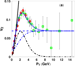
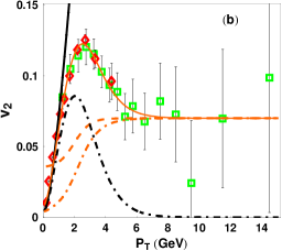
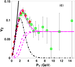
The transverse momentum () dependence of the elliptic anisotropy, , as depicted in Fig. 1 shows a rise at low towards a maximum at , and a constant value for large transverse momenta. At present the rise at low transverse momentum () is thought to be due to collective hydrodynamic expansion, which translates the initial spatial anisotropy into a anisotropy Ollitrault:1992bk over a wide region in pseudo-rapidity.
At very high , on the other hand, is believed to result from the different attenuation of hard partons (jet quenching) in the asymmetrically distributed matter Shuryak:2001me ; Gyulassy:2000gk ; Liao:2008dk . In this case the elliptic anisotropy, , is non-collective in the sense that it is due to jet-like processes which are rather local in rapidity Noncollectivity . The transition from collective (hydrodynamic) to non-collective (jet-like) anisotropy is expected to take place around , but the details are not well understood. In addition, one would expect that the attenuation of the jets should result in local, non-collective anisotropy also at lower , since the debris from the jet-quenching process needs to go somewhere. If there is indeed a sizeable non-collective contribution to at low , comparisons of (viscous) hydrodynamics with the data may lead to wrong conclusions about the viscosity of the produced matter in these collisions. Therefore, it would be desirable to have a direct measurement not only of the scale at which the transition from collective to non-collective occurs, but also of the contribution of non-collective effects in the low region, .
It is the purpose of this work to propose an observable which will distinguish between the collective and the non-collective contributions to the elliptic anisotropy. In this paper, for illustration purposes, we will identify the collective component with hydrodynamic flow and the non-collective one with attenuated jets. We note that there may be other mechanisms at work which generate similar collective and/or non-collective contributions to the elliptic anisotropy, and the proposed observable is not sensitive to any specific mechanism.
The key observation is the following: consider two rapidity bins, one forward, one backward, with a suitable separation (gap) in between. In a given event, the elliptic anisotropy of the collective component in both rapidity bins is highly correlated. The non-collective component, on the other hand, generates an elliptic anisotropy in either the forward bin or the backward bin, but never in both, resulting in very small backward-forward correlations. To illustrate this point, consider hydrodynamic expansion as an example for the collective component. In each event the elliptic anisotropy is aligned in azimuth and of comparable magnitude in the forward and backward bins. Contrast this with the elliptic anisotropy due to quenched jets, as an example for a non-collective component. At RHIC energies one rarely has more than one hard process per event. In addition, the anisotropy due to attenuated jets will be very local in rapidity and, therefore, will either contribute to the forward or to the backward bin but not to both. Consequently, these processes do not give rise to long-range forward-backward correlation of the elliptic anisotropy. At higher energies, such as the Large Hadron Collider (LHC) with many hard processes per event one has to choose a suitable rapidity gap, which is larger than typical jet cone extension but smaller than average jet-jet separation. After these general considerations, we will proceed to define the proposed observable and demonstrate its sensitivity to the degree of collectivity in contributions to .
Let us start by recalling the definition of :
| (1) |
In the above is the distribution of the event-averaged -differential yield over the azimuthal angle which is defined with respect to the reaction plane. The numerator, denoted as , may be referred to as the total elliptic anisotropy. Here we assume that the reaction plane is determined with high accuracy as it is achieved by current RHIC experiments. The particle yield at RHIC can be attributed to two main sources: the bulk matter which dominates low regime and exhibits collective flow, and the (partially suppressed) hard jets dominant at high . Both sources contribute to the total yield and thus to the measured .
The proposed new observable is the correlation of the total between forward (F) and backward (B) rapidity bins, specifically
| (2) |
where the total elliptic anisotropy in the forward, , and backward, , are defined as
| (3) | |||||
| (4) | |||||
Here we denote by the -differential particle yield for a given interval in the bins, respectively. The forward/backward bins should be chosen such that the gap is sufficiently wide to prevent a jet from contributing to both simultaneously while still keeping both bins within the “flat plateau” near mid-rapidity.
The total yield, , can be decomposed into two componentsGyulassy:2000gk , the hydrodynamic flow yield and the jet-related yield, respectively:
| (5) |
(In the following we drop the “” subscript.)
To quantify the main idea, we express the yields in the bins in each event as:
| (6) | |||
| (7) |
In the above we have introduced three random variables to schematically describe the fluctuations from event to event. represent (independent) random deviations from the average hydro flow yield in F/B bins, and satisfy . The variable assumes values of either or in each event with equal probability, i.e. while . The physical idea is that in each event there is at most one high hadron cluster contributing to the final observed anisotropy Adler:2006bw either in the forward or the backward rapidity bin. Calculations of dijet production at RHIC energy show a rapid decrease of cross section with increasing rapidity separationSzczurek:2007ep . Also with a hard trigger in one bin, the back jet is strongly degraded in a heavy ion collision, inducing negligible contribution to . In contrast, the hydrodynamic flow (ideal or viscous) contribution to the anisotropy is about equally split between F/B. The so-called anti-flowAntiflow gives rise to correlations between rapidity and in-plane . Its magnitude, , at RHIC energies is at most a few percentVoloshin:2008dg ; Antiflow and induces a correction to of the order . Furthermore it contributes equally to in both the F/B bins due to its (anti-)symmetry with respect to .
Next we introduce an interpolation function:
| (8) |
with and giving the relative weight of the jet (non-collective) and hydro flow (collective) contribution to the total, , yield, respectively. Given this function we express the observed in the bins via (1) in terms of the flow and jet contributions:
| (9) |
with defined as in (1) with the corresponding hydro-flow-only/jet-only yields. Combining (3,4,6,7,8,Exposing the non-collectivity in elliptic flow) and using the formalism of Koch , we find for Eq.(2):
| (10) |
A distinct feature is that as (hydro dominance) while in the other limit, (jet dominance). Thus, the correlation distinguishes between collective and non-collective contributions and exposes the transition from the flow to the jet regime.
In order to demonstrate the sensitivity of we study three different scenarios within a simple model. All the scenarios employ the same blast-wave model for the collective flow contribution, but they differ in the -dependence of the jet-only elliptic anisotropy, , which is not known for small . The relative strength, , of flow and jet contributions is obtained by fitting the data of the PHENIX collaboration Adler:2003kt ; Adler:2006bw ; phenix_prel for AuAu centrality class at (see Fig.1). Scenario (a) assumes a constant (see Fig.1(a)) . Scenarios (b) (Fig.1(b)) and (c) (Fig.1(c)) assume a constant for large which drops to half its value at for scenario (b) and to zero for scenario (c). For both scenarios the momentum scale at which changes towards the values at low is .
The blast-wave model for the collective hydro flow contribution we adopt from ref. Teaney:2003kp . By parameterizing the flow velocity field at freeze-out as in Teaney:2003kp we have,
| (11) |
The elliptic anisotropy is intrinsically built in the flow field : in coordinates ,, . The blast-wave parameters are chosen as , , , , , and which approximately reproduces the yield at low Adler:2006bw . Given this model we calculate the flow-only via (1) using the yield in (11) (black solid lines in Fig.1(a,b,c)). We also show the weighted flow contribution as the black dash-dot lines.
In order to model the anisotropic jet attenuation we write the jet-related yield as
| (12) |
where parameterizes the resulting azimuthal anisotropy. While the experimental data indicate to be sizeable (7%) and rather constant for phenix_prel , it is not clear how behaves at lower . To explore this we study the three scenarios described above which we parameterize as follows:
| (13) |
The three scenarios (a), (b), and (c) correspond to , , and , with the respective plotted in Fig.1 as colored long-dashed lines.
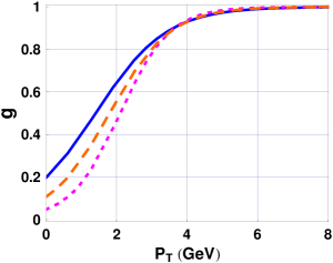
Finally, we parameterize the interpolation (8) as:
| (14) |
The parameters (in units ) are obtained by fitting of Eq.(Exposing the non-collectivity in elliptic flow) to the data for . The best choices for the three scenarios are: (a) , ; (b) , ; (c) , . In all cases a reasonable model description of the data is established over the whole range, as can be seen in Fig.1. The resulting interpolation are plotted in Fig.2. At low to intermediate they differ considerably in the magnitude of the non-collective component. Of course the plotted curves are only examples for what may happen. To quantify more experimental information will be required. We note, that an admixture of a smaller jet- seems a plausible alternative to viscous corrections for a reduced at low to intermediate .
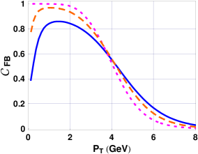
Given the above parametrization we can calculate the proposed correlation using (10). The results are shown in Fig.3. While all three cases produce similar , they are readily distinguishable by in the low to intermediate region. The non-monotonic structure seen for scenarios (a) and (b) is due to interplay between a non-vanishing jet contribution and rapidly rising hydro flow contribution to at low , which is absent in case (c). In addition, the deviation from unity at low provides a measure for the non-collective contribution to in this region and their growth with increasing . While the curves in Fig.3 depend on the specific parametrization, they demonstrate the sensitivity of to the non-collectivity which may hide in .
In summary, we have proposed to use backward-forward correlations of the elliptic anisotropy to distinguish the collective (flow) from non-collective (jet) contributions to . Using a two-component parametrization, we have studied the sensitivity of this observable to the degree of non-collectivity. We have further demonstrated that this observable is capable of exposing the transition from collective flow to jets with increasing .
Concerning an actual measurement, one issue is that even though the anisotropy of the hydro flow field is perfectly aligned in the F/B bins, the actual of produced particles in the two bins may deviate (both in magnitude and in orientation) from the supposed “” due to statistical fluctuation (see e.g. Ollitrault:1993ba ). This will reduce the correlation from unity even for purely hydro flow, with the effect scaling as . The other issue relates to the low yield in each event from intermediate to high which may cause the correlation to vanish trivially. These problems may be partially cured by selecting proper bin size and/or event trigger. Also those effects are small at low region, where the particle abundance is large.
To conclude, a measurement of will reveal the magnitude of the non-collective contribution to and the transition pattern of between collective and non-collective behavior. The centrality dependence of this transition pattern would be of interest, as the flow and jet components scale differently with centrality. In addition, these measurements will help to understand the origin of the decreasing at intermediate and constrain viscous corrections to the hydrodynamic evolution.
We thank M. Ploskon and A. Poskanzer for discussions on the experimental aspects of the proposed observable. This work is supported by the Director, Office of Energy Research, Office of High Energy and Nuclear Physics, Divisions of Nuclear Physics, of the U.S. Department of Energy under Contract No. DE-AC02-05CH11231.
References
- (1) J. Adams et al. [STAR Collaboration], Nucl. Phys. A 757, 102 (2005). K. Adcox et al. [PHENIX Collaboration], Nucl. Phys. A 757, 184 (2005). I. Arsene et al. [BRAHMS Collaboration], Nucl. Phys. A 757, 1 (2005). B. B. Back et al., Nucl. Phys. A 757, 28 (2005).
- (2) S. A. Voloshin, A. M. Poskanzer and R. Snellings, arXiv:0809.2949 [nucl-ex].
- (3) D. Teaney, J. Lauret and E. V. Shuryak, Phys. Rev. Lett. 86, 4783 (2001). P. F. Kolb, P. Huovinen, U. W. Heinz and H. Heiselberg, Phys. Lett. B 500, 232 (2001).
- (4) L. P. Csernai, J. I. Kapusta and L. D. McLerran, Phys. Rev. Lett. 97, 152303 (2006).
- (5) R. A. Lacey et al., Phys. Rev. Lett. 98, 092301 (2007)
- (6) P. Romatschke and U. Romatschke, Phys. Rev. Lett. 99, 172301 (2007); H. Song and U. W. Heinz, Phys. Lett. B 658, 279 (2008); K. Dusling and D. Teaney, Phys. Rev. C 77, 034905 (2008). Z. Xu, C. Greiner and H. Stocker, Phys. Rev. Lett. 101, 082302 (2008). H. B. Meyer, Phys. Rev. D 76, 101701 (2007).
- (7) P. Kovtun, D. T. Son and A. O. Starinets, Phys. Rev. Lett. 94, 111601 (2005).
- (8) J. Y. Ollitrault, Phys. Rev. D 46, 229 (1992).
- (9) E. V. Shuryak, Phys. Rev. C 66, 027902 (2002).
- (10) M. Gyulassy, I. Vitev and X. Wang, Phys. Rev. Lett. 86, 2537 (2001). X. Wang, Phys. Rev. C 63, 054902 (2001).
- (11) J. Liao and E. Shuryak, Phys. Rev. Lett. 102, 202302 (2009); Phys. Rev. C 75, 054907 (2007); Phys. Rev. Lett. 101, 162302 (2008); Phys. Rev. D 73, 014509 (2006).
- (12) The Mach Cone shockwaves associated with attenuated jets, though hydrodynamic, are relatively localized in rapidity, and thus “non-collective” in the present context.
- (13) S. S. Adler et al. , Phys. Rev. C 76, 034904 (2007).
- (14) A. Szczurek et al. , arXiv:0706.3438 [hep-ph].
- (15) L. P. Csernai and D. Rohrich, Phys. Lett. B 458 (1999) 454. J. Brachmann, et al. Phys. Rev. C 61 (2000) 024909. G. Wang, J. Phys. G 34 (2007) S1093. M. Lisa, et al., Phys. Lett. B 489 (2000) 287, ibid. B 496 (2000) 1.
- (16) V. Koch, arXiv:0810.2520 [nucl-th].
- (17) S. S. Adler et al., Phys. Rev. Lett. 91, 182301 (2003).
- (18) S. Afanasiev et al. , arXiv:0903.4886 [nucl-ex].
- (19) D. Teaney, Phys. Rev. C 68, 034913 (2003).
- (20) J. Y. Ollitrault, Phys. Rev. D 48, 1132 (1993).
