A UV LED-based fast-pulsed photoelectron source for time-of-flight studies

Abstract

We report on spectroscopy and time-of-flight measurements using an $18\,\mathrm{keV}$ fast-pulsed photoelectron source of adjustable intensity, ranging from single photoelectrons per pulse to 5 photoelectrons per $\mu$s at pulse repetition rates of up to 10 kHz. Short pulses between $40\,\mathrm{ns}$ and $40\,\mathrm{\mu s}$ in length were produced by switching light emitting diodes with central output wavelengths of $265\,\mathrm{nm}$ and $257\,\mathrm{nm}$, in the deep ultraviolet (or UV-C) regime, at kHz frequencies. Such photoelectron sources can be useful calibration devices for testing the properties of high-resolution electrostatic spectrometers, like the ones used in current neutrino mass searches.

1 Introduction

We describe the application of ultraviolet light emitting diodes to produce photoelectrons for a calibration source at electron energies in the keV range.

Electrostatic filters with magnetic adiabatic collimation (‘MAC-E filters’) [1, 2, 3, 4, 5] have proven to be ideal instruments for neutrino mass searches based on high-precision measurements of the tritium beta decay spectrum near the endpoint [6, 7, 8, 9]. The upcoming Karlsruhe Tritium Neutrino experiment (KATRIN) [8] aims at increasing the sensitivity on $m(\nu_{\mathrm{e}})$ by an order of magnitude with respect to its predecessors. This requires an electron spectrometer with a resolving power of $E/\Delta E=2\cdot 10^{4}$, corresponding to an energy resolution of $\Delta E\lesssim 1\,\mathrm{eV}$ at the endpoint of the tritium beta spectrum ($E=18.6\,\mathrm{keV}$).

Calibration sources at these keV energies offering line widths of the order of or even below this resolution are necessary for different purposes:

For continuous monitoring of fluctuations of the retardation potential, an electron source with high stability both of the energy and the intensity is given by a nuclear/atomic standard using $17.8\,\mathrm{keV}$ conversion electrons from ^83mKr [10]. The K-shell conversion line exhibits a natural width of $\Gamma=2.7\,\mathrm{eV}$ [11], which is small enough to monitor the retardation potential, but too broad for detailed studies of the transmission properties of the MAC-E filter. Such a conversion electron source is presently being developed for KATRIN [8, 12].

However, in order to investigate the details of the transmission properties of the MAC-E filter, an electron source in the keV range is needed, which can deliver fast-pulsed electrons with a sub-eV and well-defined energy spread and tunable beam intensities between single electrons and up to $10^{5}$ electrons per second.

A pulsed electron source can serve as a means to test a particular “time-of-flight” operational mode of the MAC-E filter that turns it from a high-pass into a band-pass filter and at the same time allows a more detailed and faster characterization of its transmission properties. This idea has been introduced in [13], where a first experimental study validating the concept is described. Such a source requires a fast timing with pulse lengths $\tau$ both smaller than the time-of-flight of the electrons through the MAC-E filter and smaller than the expected variation of the time-of-flight.

Figure 1: Schematic of the experimental setup to test the photoelectron source. From left to right: vacuum chamber with photoelectron source, electrostatic filter with magnetic adiabatic guiding and detector. The details shown in the sketch include: (i) two superconducting solenoids to produce the magnetic guiding field of the MAC-E filter (ii) the electrode configuration comprising a vacuum tank on ground potential and an inner high-voltage electrode system, (iii) field-shaping air coils, (iv) the vacuum chamber of the photoelectron source (see figure 2), (v) the stainless steel cathode and (vi) an additional water-cooled coil for local enhancement of the magnetic field strength. Magnetic field lines connecting the photocathode and the detector are indicated as dashed curves. The analyzing plane of the spectrometer at $x=0$ is defined by the maximum of the retardation potential $|U_{\mathrm{spec}}|$ coinciding with the minimum magnetic field strength $B_{\mathrm{min}}$.

Figure 2: Schematic of the photoelectron source: top view of the vacuum chamber housing the disc-shaped cathode on high voltage ($U_{\mathrm{source}}$) seen edge-on. The diameter of the stainless steel disc is $D=180\,\mathrm{mm}$ and its thickness about $d=4\,\mathrm{mm}$ (with a $\varnothing 12\,\mathrm{mm}$ rounded bead at the rim to prevent field emission when high voltage is applied). The chamber is equipped with four windows, two of which are made of UV-light transmitting quartz glass that allows to illuminate the cathode with an external UV light source. Photoelectrons are accelerated in the strong electric field and later guided magnetically into the spectrometer. (The magnetic field lines are not shown.)

A potentially suitable method to set up an electron source fulfilling the abovementioned requirements is to irradiate a cathode on high voltage with narrow-band UV light. This can be realized in a simple manner using modern deep-UV light emitting diodes (LEDs). Typical work functions $\Phi$ of metals lie in the range of about $4.2\,\mathrm{eV}$ (Ag) to $5.1\,\mathrm{eV}$ (Au), with $\Phi=4.4(2)\,\mathrm{eV}$ [4] for stainless steel, corresponding to a wavelength of the light of $\lambda=\frac{hc}{E}\approx 282\,\mathrm{nm}$. Standard laser technology can also be used to obtain output wavelengths in the deep-UV range. However, such (high-power) laser systems are rather expensive, immobile and require particular safety installations in the laboratory. By contrast, light emitting diodes operating in the deep-UV domain are advantageous due to their versatility and ease of use, albeit offering only a fraction of the optical output power as well as inferior spectral and beam profile characteristics compared to laser systems. Certain fields of application, however, benefit from this feature of moderate and highly controllable output power combined with fast pulsing (pulse length $\tau\gtrsim 25\,\mathrm{ns}$, switching slopes of the order of a few ns, see for example references [15, 16]) at repetition rates of $(1-10)\,\mathrm{kHz}$. In the particular application of photoelectron creation, the drawback of line half-widths of the order of $\delta\lambda\approx 15\,\mathrm{nm}$ typically obtained for such LEDs can partially be compensated by an appropriate matching of the work function $\Phi$ of the photocathode material and the photon energy $E_{\mathrm{photon}}$. If $\Phi$ and $E_{\mathrm{photon}}$ are chosen such that only photons from the high-energy part of the distribution can cause photoemission, the energy spread of the photoelectrons will be reduced accordingly.

In this article we will show that photoelectrons created with UV light from a pulsed LED can be used to investigate the transmission function of electrostatic electron spectrometers and to perform time-of-flight measurements. The article is structured as follows: Section 2 contains an overview of the setup and equipment used for our measurements, focusing on the photoelectron source and the retardation spectrometer. In section 3 we demonstrate the use of short UV light pulses to obtain tunable photoelectron rates. To determine the angular emission and the energy width of the photoelectron source, we measured with the MAC-E-Filter at Mainz an integrated energy spectrum and a time-of-flight spectrum, which are both presented in section 4. The paper concludes with a discussion of the results and an outlook in section 5.

2 Experimental setup

Figure 1 shows the setup used for the measurements reported on in this paper, the three main components being the photoelectron source, the electrostatic spectrometer and an electron detector.

Photoelectron source:

A sketch of the photoelectron source is presented in figure 2. The photocathode consists of a mechanically polished plane disc made of stainless steel with a diameter of $D=180\,\mathrm{mm}$ and a thickness of $d=4\,\mathrm{mm}$, encased in a cylindrical vacuum chamber with an inner diameter of $200\,\mathrm{mm}$. Stainless steel was selected as the cathode material because of its easy handling and ready machinability, as well as its work function of $\Phi=4.4(2)\,\mathrm{eV}$, which is just within the photon energy reach of commercially available UV LEDs. As light sources we employed UV LEDs of the type T9B26C and T9B25C from Seoul Semiconductor Co., Ltd, with central wavelengths of $\lambda_{\mathrm{central}}=265\,\mathrm{nm}$ and $257\,\mathrm{nm}$ at a spectral width of $\Delta\lambda_{\mathrm{FWHM}}=15.3\,\mathrm{nm}$ and $13.8\,\mathrm{nm}$, respectively (compare measured light spectra in figure 3). The LEDs provide a maximum cw optical power output of $P_{\mathrm{opt}}\leq 400\,\mathrm{\mu W}$ (T9B26C) and $P_{\mathrm{opt}}\leq 150\,\mathrm{\mu W}$ (T9B25C) [17, 18], and each is equipped with a focusing ball lens. The energy spread derived from the width of the UV light peak is $\mathrm{FWHM}=0.27\,\mathrm{eV}$ for the 265 nm LED at a central energy of $4.68\,\mathrm{eV}$ and $\mathrm{FWHM}=0.26\,\mathrm{eV}$ for the 257 nm LED at a central energy of $4.82\,\mathrm{eV}$. By comparing this with the work function of stainless steel of $4.4(2)\,\mathrm{eV}$ it is apparent that the low-energy part of the UV light may be cut off by the work function. However, the photocathode surface was not especially prepared and the vacuum at the photocathode of $p\lesssim 5\cdot 10^{-9}\,\mathrm{mbar}$ was not good enough to guarantee the homogeneity of the work function of the photocathode. In section 4 we determine the energy width of the photoelectrons to be compatible with a Gaussian standard deviation of about 0.2 eV, which matches the numbers of the expected work function inhomogeneity of 0.2 eV and energy width of the incident photons.

Figure 3: Spectra of deep-UV LED type T9B25C ($\diamond$) and T9B26C ($\bullet$), recorded with a grating spectrograph and a silicon PIN diode. In addition to the ultraviolet peak, a less intense emission component of visible light is present (not shown). This measurement was made at $I_{\mathrm{LED}}=12\,\mathrm{mA}$ (continuous operation of the LED).

Figure 4: Circuit for driving the UV LED via the function generator (AFG). The voltage $U_{\mathrm{AFG}}$ is supplied to the UV LED in series with a resistor of $R=90\,\mathrm{\Omega}$. The voltage at the UV LED $U_{\mathrm{LED}}$ was typically $5\,\mathrm{V}$ to $7.6\,\mathrm{V}$. The corresponding current was measured via the voltage drop across the resistor $R$ and varied between $I_{\mathrm{LED}}<1\,\mathrm{mA}$ and $I_{\mathrm{LED}}\approx 20\,\mathrm{mA}$ in pulsed operation of the LED.

The UV LED was supplied with pulses of varying amplitude and width $\tau$, with rise/fall times of $\leq 5\,\mathrm{ns}$, from a function generator Tektronix AFG 3102 (figure 4). The light intensity was controlled by the voltage $U_{\mathrm{LED}}$. The number of photoelectrons that were produced per pulse was determined by the interplay of $U_{\mathrm{LED}}$ and $\tau$. The UV LED was placed in front of a UV-transparent window outside the vacuum chamber. The resulting large distance of $\approx 17\,\mathrm{cm}$ between the LED position and the photocathode caused a widening of the UV light beam and a rather large spot size of area $\approx 2\,\mathrm{cm^{2}}$ on the cathode, as the spacing was not matched to the focal length of the ball lens (see figure 2). A residual gas pressure of $p\lesssim 5\cdot 10^{-9}\,\mathrm{mbar}$ inside the vacuum chamber containing the photoelectron source was maintained by means of a turbomolecular pump. The combination of the spectrometer solenoids (see next paragraph) and an additional water-cooled copper coil allowed us to vary the magnetic field strength $B_{\mathrm{source}}$ at the location of the photocathode between $\sim 0.02\,\mathrm{T}$ and $\sim 0.03\,\mathrm{T}$.

High-resolution spectrometer and electron detector:

The electron spectrometer of the Mainz neutrino mass experiment [4] was used for our measurements. This spectrometer of MAC-E filter type consists of an electrostatic retardation filter combined with an inhomogeneous magnetic guiding field. Figure 1 shows the two superconducting solenoids, which produce a strong magnetic field $B_{\mathrm{max}}$ that is attenuated towards the center of the spectrometer ($x=0$ in figure 1) by about 4 orders of magnitude to a minimum value $B_{\mathrm{min}}$ (an air coil system helps to increase the field homogeneity). This results in an expansion of the magnetic flux tube, visualized in figure 1 by a widening of the magnetic field lines. Electrons starting from a source in a higher magnetic field will spiral around the magnetic field lines. As the magnetic field strength continuously decreases towards the center of the spectrometer, the cyclotron component $E_{\perp}$ of the kinetic energy will be reduced and transformed into longitudinal kinetic energy $E_{\parallel}$ according to the relation

$$\mu=\frac{E_{\perp}}{B}=\mathrm{const.}$$ (1)

stating that, in the adiabatic limit, the orbital magnetic moment $\mu$ of the electron is a conserved quantity.

We see that the energy component $E_{\parallel}$, which is analyzed by an electrostatic retardation potential $U_{\mathrm{spec}}$, is maximized when the magnetic field reaches its minimal value $B_{\mathrm{min}}$ in the so-called “analyzing plane” ($x=0$ in figure 1). Only those electrons with sufficient axial kinetic energy, $E_{\parallel}>qU_{\mathrm{spec}}$, with $q=-e$ being the electron charge, will be able to pass the filter and get re-accelerated towards the detector at the exit of the spectrometer. The energy resolution $\Delta E$ of the MAC-E filter thus follows directly from equation (1) by assuming that an electron starts at $B_{\mathrm{max}}$ with a kinetic energy $E_{\mathrm{kin}}$ that resides entirely in the cyclotron component. In this case, $\Delta E$ corresponds to the amount of transverse energy $(E_{\perp})_{\mathrm{A,\,max}}$ that is left at the electrostatic analyzing plane of the filter after the adiabatic transformation according to equation (1):

$$\Delta E=(E_{\perp})_{\mathrm{A,\,max}}=E_{\mathrm{kin}}\cdot\frac{B_{\mathrm{min}}}{B_{\mathrm{max}}}.$$ (2)

The electrode system comprises a vacuum tank on ground potential, a set of several cylindrical retardation electrodes on negative high voltage, and a grid electrode made of wires [20]. In our measurements, the magnetic field inside the superconducting solenoids was set to $B_{\mathrm{max}}=6\,\mathrm{T}$, while the field strength $B_{\mathrm{min}}$ in the analyzing plane of the spectrometer was tuned to values between $0.3\,\mathrm{mT}$ and $0.5\,\mathrm{mT}$ using the air coil system. Inserting the values into equation (2), these settings result in an energy resolution for $18\,\mathrm{keV}$ electrons of $\Delta E\approx 1\,\mathrm{eV}$ or $\approx 1.5\,\mathrm{eV}$, respectively.

Since the energy selection is performed by the electrostatic filter, the electron detector merely serves as a counter to measure an integrated spectrum of electrons overcoming the retardation potential at a specific filter threshold $qU_{\mathrm{spec}}$. We chose a windowless Si-PIN diode (type Hamamatsu S3590-06) of size $9\times 9\,\mathrm{mm}^{2}$ as electron detector. The magnetic field at the location of the detector was $B_{\mathrm{det}}=0.34\,\mathrm{T}$. Since the magnetic field at the plate of the photocathode was $0.02-0.03\,\mathrm{T}$, the conservation of the magnetic flux requires that an area of $9-14\,\mathrm{cm}^{2}$ of the plate was imaged onto the detector. This is significantly larger than the area of $2\,\mathrm{cm^{2}}$ which is illuminated by the UV LED. Therefore it can be assumed that all photoelectrons will be imaged onto the detector. The detection efficiency is close to 100 % for the following reasons: a) The photoelectrons impinge on the Si-PIN diode with an energy of 18 keV giving a charge signal well above the noise level, b) the dead layer of this Si-PIN diode is so small that the electrons only lose about 0.5 keV there, c) photoelectrons backscattered in the detector will be reflected back to the detector by the magnetic mirror and the electric potential barrier of the MAC-E filter and thus eventually deposit all of their energy in the detector.

Data acquisition and analysis methods:

We recorded the signal of the preamplifier of the Si-PIN diode with a Flash-ADC system (Struck SIS3301-105 FADC, 14 bit, 100 MHz, 10 ns sampling width), which was triggered by the UV LED control pulse from the function generator. These digitized signals were first digitally filtered using a Butterworth bandpass filter with lower and upper filter cutoff frequencies of $1\,\mathrm{kHz}$ and $1\,\mathrm{MHz}$, respectively, and subsequently differentiated. The differential filtered signals were then analyzed for electron events. Events with a time separation smaller than $755\,\mathrm{ns}$ were counted as coincident events. For single electron events the time resolution was $\Delta t_{\mathrm{DAQ,\,analysis}}\approx 60\,\mathrm{ns}$.

3 Generation of few or single photoelectrons from short UV pulses

In order to check the usability of these photoelectrons for a characterization of the properties of MAC-E filters, the statistics of photoelectron creation was investigated. Main questions are

• how many photoelectrons are created, and how is their number influenced by the operating parameters of the UV LED,

• what is the multiplicity distribution of the detected photoelectrons, and especially

• what is the total yield of single electrons in one pulse and what is their relative fraction.

Figure 5 shows an example of the energy distribution of photoelectrons reaching the detector when the MAC-E filter is in transmission, i.e., its threshold is lower than the kinetic energy of the photoelectrons ($qU_{\mathrm{spec}}<qU_{\mathrm{source}}$). The pulse width of the UV LED was $\tau=200\,\mathrm{ns}$ at a voltage of $U_{\mathrm{LED}}=7.6\,\mathrm{V}$. For $n$ coinciding photoelectrons, an energy equivalent to $E^{n}_{\mathrm{photoel.}}=n\cdot qU_{\mathrm{source}}$ will be measured. In the depicted case electron multiplicities $n$ up to $n=4$ can be distinguished. However, single electrons are dominating at these settings. By increasing or decreasing the forward current of the LED the number of produced photoelectrons as well as their multiplicity distribution can be varied and sufficiently many electrons can be created for high statistics measurements with the MAC-E filter (figure 6(a)).

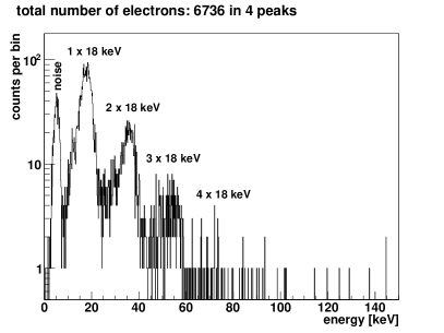
Figure 5: Photoelectron spectrum measured with the Si-PIN diode (surplus energy $E_{\mathrm{surplus}}=q(U_{\mathrm{source}}-U_{\mathrm{spec}})=18.0\,\mathrm{keV}-17.943\,\mathrm{keV}=0.057\,\mathrm{keV}$). Applied LED voltage $U_{\mathrm{LED}}=7.6\,\mathrm{V}$, pulse width $\tau=200\,\mathrm{ns}$, and repetition rate $1\,\mathrm{kHz}$. Electrons are detected at the energy $E_{\mathrm{photoel.}}^{\mathrm{single}}=qU_{\mathrm{source}}$ corresponding to the potential supplied to the photocathode, and at various multiples of this energy, $E^{n}_{\mathrm{photoel.}}=n\cdot qU_{\mathrm{source}}$. This is due to the fact that at high electron flux the time resolution is not sufficient to resolve single electrons arriving quasi-simultaneously. For the calibration the energy loss in the deadlayer of the Si-PIN diode of about $0.5\,\mathrm{keV}$ was neglected.

For advanced investigations of the transmission properties of MAC-E filters we explored the possibility of time-of-flight (ToF) studies. For this purpose single electrons with well defined energy and starting time are needed. Figure 6(b) shows the average number of photoelectrons created by the UV LED per pulse for short pulse widths at a voltage of $U_{\mathrm{LED}}=7.6\,\mathrm{V}$. Even at a very short pulse width of $40\,\mathrm{ns}$ photoelectrons are still emitted. The count rate for single electrons only is shown in figure 7(a). For the small pulse widths a plateau can be seen after an initial increase of the number of emitted single electrons. Note that the number of single photoelectrons depends on the minimal time difference needed to resolve to photoelectrons by our detector and data acquisition system, which in our case amounts to $755\,\mathrm{ns}$.

In figure 7(b) it can be verified that for the shortest pulse widths all emitted electrons come as single electrons, albeit at a small rate. If higher electron multiplicities can be tolerated then higher count rates of single electrons per pulse can be achieved. The multiplicity distribution is shown in figure 8 (top) for pulse widths up to $1\,\mathrm{\mu s}$. The average multiplicity increases for longer pulse widths. The multiplicity distributions are in reasonable agreement with Poisson statistics (figure 8, bottom).

(a) $U_{\mathrm{LED}}$ varied, $\tau=40\mu\mathrm{s}$

(b) $\tau$ varied, $U_{\mathrm{LED}}=7.6\mathrm{V}$

Figure 6: Number of photoelectrons as a function of driving voltage $U_{\mathrm{LED}}$ supplied to the UV LED (a) and as a function of the pulse width $\tau$ (b), both at a pulse repetition rate of $1\,\mathrm{kHz}$ and $E_{\mathrm{surplus}}=0.08\,\mathrm{keV}$. At $\tau=0.1\,\mathrm{\mu s}$ the alignment of the UV LED was changed, as indicated by the change of symbols (circles and squares, respectively) in figure 6(b).

(a) Single electron count rate

(b) Single electron fraction

Figure 7: Total number (a) and relative fraction (b) of single photoelectrons per pulse as a function of pulse width $\tau$, measured with $U_{\mathrm{LED}}=7.6\,\mathrm{V}$. At $\tau=0.1\,\mathrm{\mu s}$ the alignment of the UV LED was changed, as indicated by the change of symbols (circles and squares, respectively) in both figures.

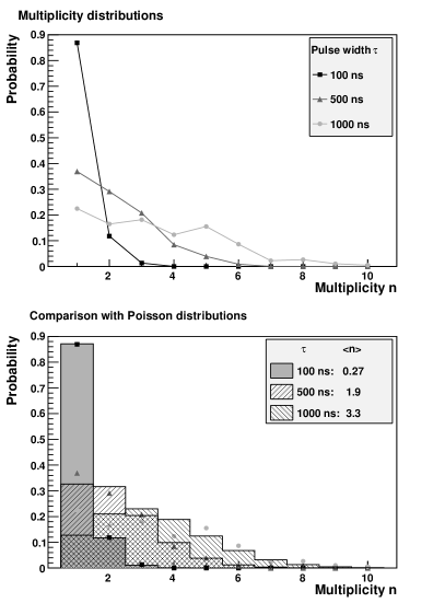
Figure 8: Multiplicity distributions for selected pulse widths: probability for a measured event to contain $n$ electrons (top). The multiplicity distributions are roughly described by a Poisson distribution (bottom: symbols represent the measured data as in the figure at the top, Poisson distributions are described by histograms). $\langle n\rangle$ denotes the average multiplicity. The UV LED was operated with $U_{\mathrm{LED}}=7.6\,\mathrm{V}$.

4 Determination of the energy distribution and the angular emission of the photoelectrons at 18 keV

As mentioned above, a time-of-flight measurement requires the energy spread of the photoelectrons to be sufficiently narrow. In order to verify this experimentally the photoelectron spectrum was measured using the MAC-E filter. The 265 nm LED was used for this measurement. By varying the retardation potential $U_{\mathrm{spec}}$ at fixed photocathode potential $U_{\mathrm{source}}$, several spectra of the photoelectron energy were recorded. For each measurement point the detected photoelectron count rate was determined by weighting the counts of each electron peak in the energy spectrum according to its multiplicity $n$. Figure 9 shows the total photoelectron count rate as a function of the surplus energy $E_{\mathrm{surplus}}=q\,(U_{\mathrm{source}}-U_{\mathrm{spec}})$ above the filter threshold. The width of this spectrum is compared with the nominal energy resolution of $\Delta E=1.5\,\mathrm{eV}$ of the MAC-E filter, which is defined for a monoenergetic electron source filling the full forward solid angle. The experimentally observed width may differ due to two main contributions:

• The observed width is smaller, since the electrons do not fill the full forward solid angle: If the angular distribution at the point of highest magnetic field $B_{\mathrm{max}}$, i.e., in the first superconducting magnet, would fill the full forward solid angle (e.g. for an isotropically emitting radioactive source), then the residual cyclotron energy in the analyzing plane (and thus the non-analyzable fraction of the energy) would be $\Delta E=1.5\,\mathrm{eV}$, which is defined as the nominal resolution of the MAC-E filter. However, in our case, we do not expect that the angular distribution in the high magnetic field is filling the full forward solid angle since the photoelectrons emitted at the photocathode are immediately accelerated by the applied potential of $18\,\mathrm{kV}$ along the E-field axis, and the B-field is nearly collinear with the E-field. Anyway, in the adiabatic case the cyclotron motion of the electron around a magnetic field line averages out any transverse electrical field. Therefore, no transverse energy is picked up and the maximum angle is of order $\theta_{\mathrm{max}}\approx\arctan\left(\sqrt{\frac{0.5\,\mathrm{eV}}{18\,\mathrm{keV}}}\right)=0.3\,\mathrm{{}^{\circ}}$, assuming a maximum initial transversal energy of order $0.5\,\mathrm{eV}$. Due to the transformation of parallel into transverse energy according to equation (1) when going from $B_{\mathrm{start}}\approx 0.02\,\mathrm{T}$ at the location of the photoelectron source to the high field of $B_{\mathrm{max}}=6\,\mathrm{T}$ in the magnet this angle corresponds to a maximum angle in the high field of $\approx 5\,\mathrm{{}^{\circ}}$, which is far from the full forward solid angle case.

• The observed width may be even larger than expected from the filled forward solid angle due to an energy spread of the electrons. In our case, the photoelectrons obtain different energies due to the finite width of the photon energy ($\mathrm{FWHM}=0.27\,\mathrm{eV}$) and the local inhomogeneity of the work function of the photocathode, A further broadening of the measured energy width may originate from potential energy losses of the electrons inside the photocathode and the ripple of the high-voltage power supplies (${\mathcal{O}}(100\,\mathrm{mV})$).

These two contributions to the width will result in different shapes of the energy spectrum. Calculations of the energy spectrum for two cases are also shown in figure 9: The dashed line illustrates the transmission function of a MAC-E filter for an isotropically emitting but monoenergetic electron source. The full line shows the expected transmission function for a single angle electron source with emission along the normal of the photocathode ($\theta=0\,\mathrm{{}^{\circ}}$) having an initial energy spread of the photoelectrons described by a Gaussian broadening with $\sigma_{\mathrm{energy}}=0.21\,\mathrm{eV}$. The latter curve fits much better to the data.

Although the small number of our data points and their limited statistics do not allow to really deconvolve the energy distribution of our photoelectron source, we can state that our data are well described by assuming that the photoelectrons are created with an energy spread of just $\sigma_{\mathrm{energy}}=0.21\,\mathrm{eV}$ and that their momentum vector is nearly parallel to the magnetic field lines after acceleration. Fitting these assumptions (Gaussian energy distribution and no angular spread) to the data yields a fit error for the Gaussian spread of $\Delta\sigma_{\mathrm{energy}}=\pm 0.02\,\mathrm{eV}$

Figure 9: Measured integral energy spectrum of photoelectrons. Also shown are two calculations for monoenergetic and isotropic photoelectron emission (dashed line) and for photoelectrons emitted along the normal of the photocathode but with a Gaussian energy spread of $\sigma_{\mathrm{energy}}=0.21\,\mathrm{eV}$ (solid line). The measurement is consistent with the latter.

This small energy spread and narrow angular distribution of the photoelectrons, together with pulse lengths shorter than $100\,\mathrm{ns}$ and a fast data acquisition system with a time resolution of $\Delta t_{\mathrm{DAQ,\,analysis}}\approx 60\,\mathrm{ns}$ for single electrons, allows us to perform a high-resolution determination of the time of flight for photoelectrons passing the MAC-E filter at different surplus energies. Expected time-of-flight values range between $\approx 200\,\mathrm{ns}$ for surplus energies of $500\,\mathrm{eV}$ to several microseconds at few eV.

To obtain this time-of-flight spectrum we analyzed the data taken for the scan of the energy spectrum of the photoelectrons with respect to the arrival time distributions of the electrons. The start signal for the measurement of arrival times was provided by the trigger output of the function generator powering the UV LED. This control signal was recorded on the second channel of the Flash-ADC card. The stop time was given by the time of an electron signal from the detector preamplifier recorded in the first channel of the Flash-ADC.

Figure 10 presents the time-of-flight spectrum for photoelectrons over a wide range of surplus energies above the filter potential using the mean time of flight for each surplus energy. Electrons with large surplus energies $qU_{\mathrm{source}}-qU_{\mathrm{spec}}=E_{\mathrm{surplus}}\approx 410~{}\mathrm{eV}$ reach the detector about $220\,\mathrm{ns}$ after the UV light pulse irradiated the photocathode, whereas electrons with small energies of $E_{\mathrm{surplus}}\approx 1.7~{}\mathrm{eV}$ arrive after about $4\,\mathrm{\mu s}$. The measurement is described well by a calculation based on

$$t_{\mathrm{stop}}-t_{\mathrm{start}}=\int_{x_{\mathrm{start}}}^{x_{\mathrm{stop}}}\frac{\mathrm{d}x}{v(x)}=\int_{x_{\mathrm{start}}}^{x_{\mathrm{stop}}}\sqrt{\frac{m_{e}}{2q(U_{\mathrm{source}}-U(x))}}~{}~{}\mathrm{d}x.$$ (3)

Here we assumed that the velocity of the electron is parallel to the magnetic field lines and thus defined by the gain of the kinetic energy $E_{\mathrm{kin}}$ in the electric potential $U$. This corresponds to the expectation discussed above that the photoelectrons are emitted with a negligible amount of transversal energy from the photocathode and accelerated by an electric field parallel to the magnetic field lines.

Due to the broadening of the initial photoelectron energy distribution this calculation deviates from the measurement for small excess energies. When taking the broadening into account by folding equation (3) with a Gaussian energy distribution the calculation also agrees with the measurement at small excess energies (figure 10). The best agreement is achieved for a Gaussian width of $\sigma_{\mathrm{energy}}=0.2\,\mathrm{eV}$, which matches well the Gaussian width extracted from the integral energy spectrum.

Figure 11 shows the spread of the arrival time distributions for a given surplus energy. The increase of the width of the distributions at small excess energy again reflects the effect of the spread in initial photoelectron energy.

These measurements show that with a photoelectron source based on UV light from a modern LED irradiating a stainless steel cathode the time of flight of single electrons can be determined in MAC-E filters.

Figure 10: Mean time of flight of photoelectrons passing the electrostatic filter versus surplus energy with respect to the filter potential ($E_{\mathrm{surplus}}=q(U_{\mathrm{source}}-U_{\mathrm{spec}})$) with $\tau=200\,\mathrm{ns}$ and $U_{\mathrm{LED}}=7.6\,\mathrm{V}$. (a) Comparison between measured values ($\bullet$) and values calculated according to equation (3) (solid line) over a wide range of surplus energies. (b) For large time-of-flight values, corrections due to an energy smearing of the photoelectrons become relevant. Calculations for varying widths of a Gaussian broadening of the surplus energy are shown: $\sigma_{\mathrm{energy}}=0.15\,\mathrm{eV}$ (dashed line), $0.20\,\mathrm{eV}$ (dotted line), $0.25\,\mathrm{eV}$ (dash-dotted line), and no broadening (solid line). A good agreement between measurement and calculation is achieved for $\sigma_{\mathrm{energy}}=0.20\,\mathrm{eV}$.

Figure 11: Full width at half maximum (FWHM) of the measured time-of-flight distribution of photoelectrons at different surplus energies. For $U_{\mathrm{source}}-U_{\mathrm{spec}}\ll 0$ the FWHM of the measured time-of-flight distribution is limited by the full start time uncertainty of the electrons defined by the width of the UV light pulses ($\tau=200\,\mathrm{ns}$) and by the uncertainty of the arrival time determination related to the data acquisition system.

5 Discussion of results and outlook

We have demonstrated that by using a deep-UV light emitting diode illuminating a stainless steel cathode photoelectrons, which are well-defined in energy and time, can be created with rates covering a large dynamical range. We accelerated these photoelectrons by an electric field to a typical energy of $18\,\mathrm{keV}$.

We determined the energy distribution of the photoelectrons in two ways, with both methods yielding consistent Gaussian widths of about $\sigma_{\mathrm{energy}}=0.2\,\mathrm{eV}$. This value may probably be further improved by using a cathode material with a better defined work function (e.g. a monocrystalline surface instead of stainless steel in a better vacuum). We achieved the time definition by electrically pulsing the UV LED. Pulse lengths from 40 $\mu$s down to 40 ns were applied, resulting in a corresponding definition of the photoelectron start time. To reach high total photoelectron rates we used pulse repetition rates of typically 1 kHz. By choosing the operating parameters of the UV LED like the operating voltage (and thus the forward current), pulse width and pulse repetition rate we obtained photoelectron rates from several Hz up to several 10 kHz on average, with a maximum rate during the pulse of $5\,\mathrm{electrons/\mu s}$. In particular, the operating parameters can be chosen such that only – or at least predominantly – single photoelectrons per pulse are achieved (figure 7(b)), which allows to minimize the pile-up ratio and results in very good timing (e.g., for time-of-flight measurements).

At the Mainz spectrometer (an electrostatic retardation spectrometer of MAC-E filter type) we measured the transmitted electron rate as a function of the retardation energy (integral MAC-E filter mode), and the corresponding time-of-flight of the electrons (non-integral MAC-E-TOF mode). We found that the observed integral as well as the time-of-flight spectrum agree well with the expectations considering an initial Gaussian energy width of the photoelectrons of $\sigma_{\mathrm{energy}}=0.2\,\mathrm{eV}$ (compare figures 9 and 10). These investigations were performed especially in view of an application as a test source for the large MAC-E filter of the KATRIN experiment (see Ref. [21]). The achieved line width, the small angular emittance as well as the obtained time-of-flight precision match well the requirements to determine precisely the local electric retarding potential over the $64\,\mathrm{m^{2}}$ large analyzing plane of the KATRIN main spectrometer by the onset of the transmission as well as to validate the correct evolution of the electric retarding potential along the electron trajectory by the time-of-flight method.

In a further development of this photoelectron source the additional feature of creating photoelectrons at well-defined transversal energy can be accomplished by choosing a suitable configuration of the electric and magnetic fields at the location of the photocathode. In the setup presented in this work magnetic and electric field were essentially parallel at the photocathode, resulting in electrons with negligible transversal energy. For different field configurations using a fast non-adiabatic acceleration in a strong electrical field transversal energies $>0$ can be realized. Such an electron source allows to probe the transmission properties of a MAC-E filter in much more detail (e.g., in dependence of the transversal energy and the correctness of the adiabatic transformation according to equation (1)). We will report on first experimental studies with a proof of principle in a forthcoming publication [22]. By combining fast pulsing with angular selectivity a powerful calibration tool for the KATRIN experiment and other applications may thus be achieved.

References

References

- [1] T. Hsu and J. L. Hirshfield, Electrostatic energy analyzer using a nonuniform axial magnetic field, Rev. Sci. Instrum. 47 (1976) 236
-
[2]
G. Beamson, H. Q. Porter and D. W. Turner, The collimating and magnifying properties of a superconducting field photoelectron spectrometer, J. Phys. E 13 (1980) 64;
corrigendum: J. Phys. E 14 (1981) 256;
G. Beamson, H. Q. Porter and D. W. Turner, Photoelectron spectromicroscopy, Nature 290 (1981) 556 - [3] P. Kruit and F. H. Read, Magnetic field paralleliser for electron-spectrometer and electron-image magnifier, J. Phys. E 16 (1983) 313
- [4] A. Picard et al, A solenoid retarding spectrometer with high resolution and transmission for keV electrons, Nucl. Instr. Meth. B 63 (1992) 345
- [5] V. M. Lobashev and P. E. Spivak, A method for measuring the electron antineutrino rest mass, Nucl. Instr. Meth. A 240 (1985) 305
- [6] Ch. Kraus, B. Bornschein, L. Bornschein, J. Bonn, B. Flatt, A. Kovalík, B. Ostrick, E. W. Otten, J. P. Schall, Th. Thümmler, Ch. Weinheimer, Final results from phase II of the Mainz neutrino mass search in tritium decay, Eur. Phys. J. C 40 (2005) 447
- [7] V. M. Lobashev, The search for the neutrino mass by direct method in the tritium beta-decay and perspectives of study it in the project KATRIN, Nucl. Phys. A 719 (2003) C153
- [8] The KATRIN collaboration (J. Angrik et al), KATRIN Design Report 2004, FZKA Scientific Report 7090 (2005), URL: http://bibliothek.fzk.de/zb/berichte/FZKA7090.pdf
- [9] E. W. Otten and C. Weinheimer, Neutrino mass limit from tritium beta decay, Rep. Prog. Phys. 71 (2008) 086201
- [10] A. Picard et al, Precision measurement of the conversion electron spectrum of with a solenoid retarding spectrometer, Z. Phys. A 342 (1992) 71
- [11] J. L. Campbell and T. Papp, Widths of the atomic K–N7 levels, Atomic Data and Nuclear Data Tables 77 (2001) 1
- [12] B. Ostrick, Eine kondensierte 83mKr-Kalibrationsquelle für KATRIN, Ph.D. thesis, Westfälische Wilhelms-Universität Münster, 2009, and to be published
- [13] J. Bonn, L. Bornschein, B. Degen, E. W. Otten, Ch. Weinheimer, A high resolution electrostatic time-of-flight spectrometer with adiabatic magnetic collimation, Nucl. Instr. Meth. A 421 (1999) 256
- [14] J. Deng et al, 247 nm Ultra-Violet Light Emitting Diodes, Jpn. J. Appl. Phys. 46 (2007) L263
- [15] R. Gaska and J. P. Zhang, Deep-UV LEDs: Physics, Performance and Applications, Device and Process Technologies for Microelectronics, MEMS, and Photonics IV, Proceedings of SPIE Vol. 6037 (2005) 603706
- [16] M. Shatalov et al, Time-resolved electroluminescence of AlGaN-based light-emitting diodes with emission at 285 nm, Appl. Phys. Lett. 82 (2003) 167
- [17] Seoul Semiconductor Co., Ltd., Specification document for UV LED model series T9B26*, 2006, URL: http://www.socled.com
- [18] Seoul Semiconductor Co., Ltd., Specification document for UV LED model series T9B25*, 2006, URL: http://www.socled.com
- [19] Ch. Weinheimer, M. Schrader, J. Bonn, Th. Loeken and H. Backe, Measurement of energy resolution and dead layer thickness of -cooled PIN photodiodes, Nucl. Instr. Meth. A 311 (1992) 273
- [20] B. Flatt, Voruntersuchungen zu den Spektrometern des KATRIN-Experiments, Ph.D. thesis, Johannes-Gutenberg Universität Mainz, 2004
- [21] K. Valerius, Spectrometer-related background processes and their suppression in the KATRIN experiment, Ph.D. thesis, Westfälische Wilhelms-Universität Münster, 2009
- [22] K. Valerius et al, to be published