Gamma-ray variability from wind clumping in HMXBs with jets

Abstract

In the subclass of high-mass X-ray binaries known as “microquasars”, relativistic hadrons in the jets launched by the compact object can interact with cold protons from the star’s radiatively driven wind, producing pions that then quickly decay into gamma rays. Since the resulting gamma-ray emissivity depends on the target density, the detection of rapid variability in microquasars with GLAST and the new generation of Cherenkov imaging arrays could be used to probe the clumped structure of the stellar wind. We show here that the fluctuation in gamma rays can be modeled using a “porosity length” formalism, usually applied to characterize clumping effects. In particular, for a porosity length defined by $h\equiv\ell/f$, i.e. as the ratio of the characteristic size $\ell$ of clumps to their volume filling factor $f$, we find that the relative fluctuation in gamma-ray emission in a binary with orbital separation $a$ scales as $\sqrt{h/\pi a}$ in the “thin-jet” limit, and is reduced by a factor $1/\sqrt{1+\phi a/2\ell}$ for a jet with a finite opening angle $\phi$. For a thin jet and quite moderate porosity length $h\approx 0.03\,a$, this implies a ca. 10% variation in the gamma-ray emission. Moreover, the illumination of individual large clumps might result in isolated flares, as has been recently observed in some massive gamma-ray binaries.

1. Introduction

One of the most exciting achievements of high-energy astronomy in recent years has been to establish that high-mass X-ray binaries (HMXBs) and microquasars are variable gamma-ray sources (Aharonian et al. 2005, 2006; Albert et al. 2006, 2007). The variability is modulated with the orbital period, but in addition short-timescale flares seem to be present (Albert et al. 2007, Paredes 2008). Since at least some of the massive gamma-ray binaries are known to have jets, interactions of relativistic particles with the stellar wind of the hot primary star seem unavoidable (Romero et al. 2003). At the same time, there are increasing reasons to think that the winds of hot stars have a clumped structure (e.g. Dessart & Owocki 2003, 2005; Puls et al. 2006, and references therein). The observational signatures of such clumping often just depend on the overall volume filling factor, with not much sensitivity to their scale. Here we argue that gamma-ray astronomy can provide new constraints on the clumped structure of stellar winds in massive binaries with jets. At the same time, our analysis provides a simple formalism for understanding the rapid flares and flickering in the light curves of these objects. Our basic hypothesis is that the jet produced close to the compact object in a microquasar will interact with the stellar wind, producing gamma-rays through inelastic $pp$ interactions, and that the emerging gamma-ray emission will present a variability that is related to the structure of the wind. Thus the detection of rapid variability by satellites like GLAST and by Cherenkov arrays like MAGIC II, HESS II, and VERITAS can be used as a diagnosis of the structure of the wind itself.

2. Jet-clump interactions

2.1. The general scenario

The basic scenario explored in this paper is illustrated in figure 1. A binary system consists of a compact object (e.g., a black hole) and a massive, hot star. The compact object accretes from the star and produces two jets. For simplicity, we assume that these jets are normal to the orbital plane and the accretion disk (see otherwise Romero & Orellana 2005). We also assume a circular orbit of radius $a$. The wind of the star has a clumped structure and individual clumps interact with the jet at different altitudes, forming an angle $\Psi$ with the orbital plane. The $z$-axis is taken along the jet, forming an angle $\theta$ with the line of sight, with the orbit in the $xy$-plane. The jet has an opening angle $\phi$. To consider the effects of a single jet-clump interaction, we first adopt a model for the jet (Sect. 2.2).

In addition to wind clumping, there can also be intrinsic variability associated with the jet. This includes orbital modulation, as observed in LS 5039 or LS I 61 303 (e.g., Aharonian et al. 2006; Albert et al. 2006), and periodic precession of steady jets (e.g., Kaufman-Bernadó et al. 2002). Both these long-term, periodic variations would be quite distinct from the rapid, stochastic variations from wind clumps. Intrinsic disturbances and shocks in jets can produce aperiodic variability that might be confused with variability associated with jet-clump interactions. In microquasars such intrinsic fluctuations are expected to arise in the context of the jet-disk coupling hypothesis, as proposed by Falcke & Biermann (1995) for the case of AGNs, and observationally demonstrated for a galactic microquasar by Mirabel et al. (1998). The same effect has been observed in AGNs (Marscher et al. 2002). Thus intrinsic variability in the jet would likely be preceded by a change in the accretion disk X-ray activity, whereas in the case of a jet-clump interaction, the effect should be the opposite: first the gamma-ray flare would appear, and then, an non-thermal X-ray flare produced by the secondary electrons and positrons as well as the primary electrons injected into the clump would show up. Depending on the magnetic field and the clump density, the X-ray radiation could be dominated by synchrotron, inverse-Compton, or Bremsstrahlung emission, with a total luminosity related to that of the gamma-ray flare. In summary, simultaneous X-ray observations with gamma-ray observations could be used to differenciate jet-clump events from intrinsic variability produced by the propagation of shocks in the jets.

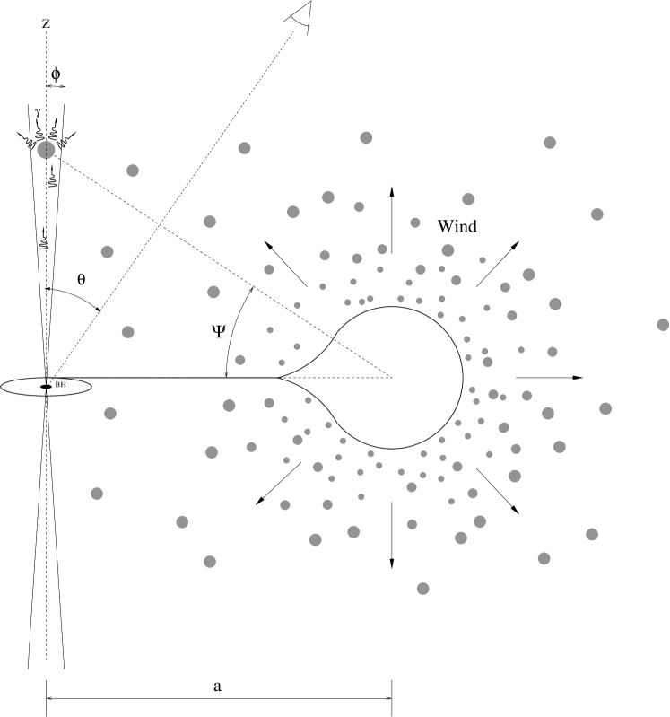
Figure 1.— Sketch of the assumed model, described further in the text.

2.2. Basics of the jet model and jet-clump interaction

The matter content of the jets produced by microquasars is not well-known. However, the presence of relativistic hadrons in the jets of SS433 has been directly inferred from iron X-ray line observations (e.g. Kotani et al. 1994, 1996; Migliari et al. 2002). In addition, the large perturbations some jets cause in the interstellar medium imply a significant baryon load (Gallo et al. 2005, Heinz 2006). The fact that the jets are usually well-collimated also favors a content with cold protons that provide confinement to the relativistic gas. We adopt here the basic jet model proposed by Bosch-Ramon et al. (2006), where the jet is dynamically dominated by cold protons. Since the jet launching likely stems from magneto-centrifugal effects (e.g., Blandford & Payne 1982), the jet magnetic field is assumed to be in equipartition with the particle energy density, with typical values of 1 kG.

Shocks from plasma collisions in the jet can produce a non-thermal relativistic particle population. But only a fraction $q_{j}\approx 0.1$ of the total jet luminosity $L_{j}\approx 10^{37}{\rm erg\,s^{-1}}$ is expected to be converted into relativistic protons by such diffusive shock acceleration at the jet base (e.g., Riegler et al. 2007). The resulting gamma-ray emission can be calculated as in Romero et al. (2003) and Orellana et al. (2007). For interaction between relativistic ($\sim$TeV) protons in the jet with cold protons in the wind, a characteristic cross section is $\sigma\approx 3.4\times 10^{-26}$ cm² (Kelner et al. 2006). For a typical wind mass loss rate ${\dot{M}}=10^{-6}M_{\odot}{\rm yr}^{-1}$ and speed $v=1000\,{\rm km\,s}^{-1}$, the characteristic wind column depth traversed by the jet from an orbital separation distance $a\sim 0.2AU\sim 3\times 10^{12}~{}$cm is $N\approx 5\times 10^{22}$ cm^-2. This implies that only a small fraction, $\tau_{w}\approx\sigma N\approx 0.002$, of relativistic particles in the jet are converted to gamma-rays by interaction with the entire wind. The leads to a mean gamma-ray luminosity of $L_{\gamma}=q_{j}\tau_{w}L_{j}\approx 2\times 10^{33}\,{\rm erg\,s}^{-1}$.

Clumps in the wind can lead to variations and flares in this gamma-ray emission. For clumps of size $\ell\approx 10^{11}$ cm, corresponding to a few percent of the stellar radius, the flow into the jet at the wind speed implies a flare timescale less than an hour. While quite short, this is comparable to the variability already detected in Cygnus X-1 by MAGIC (Albert et al. 2007). HESS II and MAGIC II will have a higher sensitivity, so these instruments should be able to detect variability from galactic sources like LS 5039, LS I +61 303 and Cygnus X-1 on timescales below an hour.

The flare brightness depends on the clump column depth and the resulting fraction of the relativistic particle luminosity converted to gamma rays. For clumps of the above size with a volume filling factor $f=0.1$, using the above wind parameters at an orbital separation distance gives a clump column $N_{c}=3\times 10^{21}{\rm cm}^{-2}$. The associated clump attenuation fraction is $\tau_{c}=\sigma N_{c}\approx 10^{-4}$, implying a flare gamma-ray brightness of $L_{\gamma}=q_{j}\tau_{c}L_{j}\approx 10^{32}\,{\rm erg\,s}^{-1}$. Stronger flares could result when a large clump crosses close to the base of the jet. Overall, if a microquasar is observed in an active state (i.e. when the jet is powerful), then satellite instruments like GLAST and ground-based Cherenkov telescopes should be able to detect variability down to timescales of $\sim 1$ h or so, sufficient to measure variations associated with jet interactions with wind clumps.

The above picture assumes that the jet is not significantly dispersed or attenuated by other interactions with the wind, for example gyro-scattering off magnetic field fluctuations in the clumps. Taking a characteristic temperature $T\approx 10^{4}$ K along with the above parameters for the wind and clumps, we can estimate that at the orbital separation distance $a=0.2$ AU, clumps have a typical thermal energy density $E_{c}=(3/2)n_{c}kT\sim 0.07\,{\rm erg\,cm}^{-3}$, with the corresponding equipartition magnetic field thus of order a Gauss. For relativistic protons of Lorentz factor $\gamma$, the associated gyroradius is just $r_{g}=30\gamma$ km. Even for TeV particles with $\gamma\approx 10^{3}$, this is much less than the clump size, $r_{g}\ll\ell$, implying that individual such particles should be quite effectively deflected by such clumps.

However, this does not mean that such gyroscattering by wind clumps can substantially disperse the jet. The simple reason is that the energy density of the jet completely overwhelms that of the wind clumps. For a jet with opening $\phi=1^{o}$ and thus solid angle $\Omega=\pi\phi^{2}\approx 10^{-3}$ ster, the energy density at an orbital distance $a$ is $E_{j}=L_{j}/(\Omega ca^{2})\approx 4\times 10^{4}{\rm erg\,cm}^{-3}$, nearly a million times higher than for the clumps. This suggests that, while clump-jet interactions may substantially perturb or even destroy the clumps, the back-effect on the jet should be very small. Moreover, while the dynamics of such clump destructions are likely to be complex, the overall exposure of clumped wind protons to interaction with the relativistic protons in the jet may, to a first approximation, remain relatively unaffected. Overall, it thus seems reasonable to assume a simple interception model of jet-wind interaction, withrelatively little dispersal or attenuation of the jet through the wind.

3. Porosity-length scaling of gamma-ray fluctuation from multiple clumps

Individual jet-clump interactions should be observable only as rare, flaring events. But if the whole stellar wind is clumped, then integrated along the jet there will be clump interactions occurring all the time, leading to a flickering in the light curve, with the relative amplitude depending on the clump characteristics. Under the above scenario that the overall jet attenuation is small, both cumulatively and by individual clumps, the mean gamma-ray emission should depend on the mean number of clumps intersected, while the relative fluctuation should (following standard statistics) scale with the inverse square-root of this mean number. But, as we now demonstrate, this mean number itself scales with the same porosity-length parameter that has been used, for example, by Owocki and Cohen (2006) to characterize the effect of wind clumps on absorption of X-ray line emission (see also Oskinova, Hamman, and Feldmeier 2006).

Let us again consider the gamma-ray emission integrated along the jet. Representing the relativistic particle component of the jet as a narrow beam with constant luminosity $L_{b}=q_{j}L_{j}$ along its length coordinate $z$, the total mean gamma-ray luminosity $L_{\gamma}$ scales (in the small-attenuation limit $L_{\gamma}\ll L_{b}$) as

$$\left\langle L_{\gamma}\right\rangle=L_{b}\sigma\int_{0}^{\infty}n(z)\,dz\,,$$ (1)

where $n(z)$ is the local mean wind density (i.e. averaged over any small-scale clumped structure), and $\sigma$ is the gamma-ray conversion cross-section defined above.

The fluctuation about this mean emission depends on the properties of any wind clumps. A simple model assumes a wind consisting entirely of clumps of characteristic length $\ell$ and volume filling factor $f$, for which the mean-free-path for any ray through the clumps is given by the porosity length $h\equiv\ell/f$. For a local interval along the jet $\Delta z$, the mean number of clumps intersected is thus $\Delta N_{c}=\Delta z/h$, whereas the associated mean gamma-ray production is given by

$$\left\langle\Delta L_{\gamma}\right\rangle=L_{b}\sigma n\Delta z=L_{b}\sigma n\Delta N_{c}h.$$ (2)

But by standard statistics for finite contributions from a discrete number $\Delta N_{c}$, the variance of this emission about the mean is

$$\left\langle\Delta L_{\gamma}^{2}\right\rangle-\left\langle\Delta L_{\gamma}\right\rangle^{2}={L_{b}^{2}\sigma^{2}n^{2}\Delta z^{2}\over\Delta N_{c}}={L_{b}^{2}\sigma^{2}n^{2}h\Delta z}\,.$$ (3)

Each clump-jet interaction is an independent process; thus, the variance of an ensemble of interactions is just the sum of the variances of the individual interactions. The total variance is then just the integral that results from summing these individual variances as one allows $\Delta z\rightarrow dz$. Taking the square-root of this yields an expression for the relative rms fluctuation of intensity,

$${\delta L_{\gamma}\over\left<L_{\gamma}\right>}={\sqrt{\int_{0}^{\infty}n^{2}h\,dz}\over\int_{0}^{\infty}n\,dz}\,.$$ (4)

Note that, in this linearized analysis based on the weak-attenuation model for the jet, the cross-section $\sigma$ scales out of this fluctuation relative to the mean.

As a simple example, for a wind with a constant velocity and constant porosity length $h$, the relative variation is just

$${\delta L_{\gamma}\over\left<L_{\gamma}\right>}=\sqrt{h/a}\,{\sqrt{\int_{0}^{\infty}dx/(1+x^{2})^{2}}\over\int_{0}^{\infty}dx/(1+x^{2})}=\sqrt{h/\pi a}\,.$$ (5)

Typically, if, say $h\approx 0.03a$, then ${\delta L_{\gamma}}/{L_{\gamma}}\approx 0.1$. This implies an expected flickering at the level of 10% for a wind with such porosity parameters, occuring on a timescale of an hour or less.

4. Gamma-ray fluctuations from a finite-cone jet

Let us now generalize this analysis to take account of a small but finite opening angle $\phi$ for the jet cone. The key is to consider now the total number of clumps intersecting the jet of solid angle $\Omega\approx\phi^{2}$. At a given distance $z$ from the black hole origin, the cone area is $\Omega z^{2}=(\phi z)^{2}$. For clumps of size $\ell$ and mean separation $L$, the number of clumps intercepted by the volume $\Omega z^{2}\Delta z$ is

$$\Delta N_{c}=\Delta z{\ell^{2}+\Omega z^{2}\over L^{3}}={\Delta z\over h}\,\left[1+(\phi z/\ell)^{2}\right]\,,$$ (6)

where the latter equality uses the definition of the porosity length $h=\ell/f$ in terms of clump size $\ell$ and volume filling factor $f=\ell^{3}/L^{3}$.

Note that the term “intercepted” is chosen purposefully here, to be distinct from, e.g., “contained”. As the jet area becomes small compared to the clump size, the average number of clumps contained in the volume would fractionally approach zero, whereas the number of clumps intercepted approaches the finite, thin-jet value, set by the number of porosity lengths $h$ crossed in the thickness $\Delta z$. As such, for $\phi z\ll\ell$, this more-general expression naturally recovers the thin-jet scaling, $\Delta N_{c}=\Delta z/h$, used in the previous subsection.

Applying now this more-general scaling, the emission variance of this layer is given by

$${L_{b}^{2}\sigma^{2}n^{2}\Delta z^{2}\over\Delta N_{c}}={L_{b}^{2}\sigma^{2}n^{2}h\Delta z\over 1+\phi^{2}z^{2}/\ell^{2}}\,.$$ (7)

Obtaining the total variance again by letting the sum become an integral, the relative rms fluctuation of intensity thus now has the corrected general form,

$${\delta L_{\gamma}\over\left<L_{\gamma}\right>}={\sqrt{\int_{0}^{\infty}n^{2}h\,dz/(1+\phi^{2}z^{2}/\ell^{2})}\over\int_{0}^{\infty}n\,dz}\,.$$ (8)

For the simple example that both the porosity length $h$ and clump size $\ell$ are fixed constants, the integral forms for the relative variation becomes

$${\delta L_{\gamma}\over\left<L_{\gamma}\right>}=\sqrt{h/a}\,{\sqrt{\int_{0}^{\infty}dx/[(1+{p}^{2}x^{2})(1+x^{2})^{2}]}\over\int_{0}^{\infty}dx/(1+x^{2})}\,,$$ (9)

where ${p}\equiv{\phi a/\ell}$ defines a “jet-to-clump” size parameter, evaluated at the binary separation radius $a$. Carrying out the integrals, we find the fluctuation from the thin-jet limit given above must now be corrected by a factor

$$C_{{p}}={\sqrt{1+2{p}}\over 1+{p}}\approx{1\over\sqrt{1+{p}/2}}\,,$$ (10)

where the latter simplification is accurate to within 6% over the full range of ${p}$.

In the thin-jet limit ${p}=\phi a/\ell\ll 1$, the correction approaches unity, as required. But in the thick-jet limit, it scales as

$$C_{{p}}\approx\sqrt{2\over{p}}=\sqrt{2\ell\over\phi a}~{}~{}~{};~{}~{}\phi\gg\ell/a\,.$$ (11)

When combined with the above thin-jet results, the general scaling of the fluctuation takes the approximate overall form

$${\delta L_{\gamma}\over\left<L_{\gamma}\right>}\approx\sqrt{h/\pi a\over 1+\phi a/2\ell}$$ (12)

wherein the numerator represents the thin-jet scaling, while the denominator corrects for the finite jet size.

If the jet has an opening of one degree, then $\phi=(\pi/180)\approx 1.7\times 10^{-2}$ radian. If we assume a clump filling factor of say, $f=1/10$, then the example of the previous section for a fixed porosity length $h=0.03\,a$ implies a clump size $\ell=0.003\,a$, and so a moderately large jet-to-clump size ratio of ${p}\approx 6$. But even this gives only a quite modest reduction factor $C_{{p}}\approx 0.5$, yielding now a relative gamma-ray fluctuation of about 5%.

The bottom line here is thus that the correction for finite cone size seems likely to give only a modest (typically a factor two) reduction in the previously predicted gamma-ray fluctuation levels of order 10%. This holds for clump scales of order a few thousandths of the binary separation, and for jet cone angles of about 1 degree. As the ratio between these two parameters decreases (still keeping a fixed porosity length), the fluctuation level should decrease in proportion to the square root of that ratio, i.e. $\delta L_{\gamma}\propto\sqrt{l/\phi}\propto 1/\sqrt{{p}}$.

5. Conclusion

Overall, for a given binary separation scale $a$, our general model for gamma-ray fluctuation due to jet interaction with clumped wind has just two free parameters, namely the porosity length ratio $h/a$, and the jet-to-clump size ratio ${p}=\phi a/\ell$. Given these parameters, then, within factors of order unity, the predicted relative gamma-ray fluctuation is given by eqn. (12). For reasonable clump properties with $h\approx 10\ell\approx 0.03a$, the fluctuation amplitude would be a few percent.

Note however that the formalism here is based on a simple model in which all the wind mass is assumed to be contained in clumps of a single, common scale $\ell$, with the regions between the clumps effectively taken to be completely empty. More realistically, the wind structure can be expected to contain clumps with a range of length scales, superposed perhaps on the background smooth medium that contains some nonzero fraction of the wind mass. For such a medium, the level of gamma-ray fluctuation would likely be modified from that derived here, perhaps generally to a lower net level, but further analysis and modeling will be required to quantify this.

One potential approach might be to adopt the “power-law porosity” formalism developed to model the effect of such a clump distribution on continuum driven mass loss (Owocki, Gayley, and Shaviv 2004). This would introduce an additional dependence on the distribution power index $\alpha_{p}$, with smaller values $\alpha_{p}\rightarrow 0$ tending to the smooth flow limit. But for moderate power indices in the range $0.5<\alpha_{p}<1$, we can anticipate that the above scalings should still roughly apply, with some reduction that depends on the power index $\alpha_{p}$, if one identifies the assumed porosity length $h$ with the strongest clumps.

Thus while there remains much further work to determine the likely nature of wind clumping from hydrodynamical models, the basic porosity formalism developed here does seem a promising way to characterize its broad effect on key observational diagnostics, including the relative level of fluctuation in the gamma-ray emission of HMXB microquasar systems.

References

- (1) Aharonian, F.A., & Atoyan, A.M., 1996, Space Sci. Rev., 75, 357
- (2) Aharonian, F.A., & Atoyan, A.M., 2000, A&A, 352, 937
- (3) Aharonian, F. A., et al. (HESS Coll.), 2005, Science, 309, 746
- (4) Aharonian, F. A., et al. (HESS Coll.), 2006, Science, 314, 1424
- (5) Albert, J. et al. (MAGIC coll.), 2006, Science, 312, 1771
- (6) Albert, J. et al. (MAGIC coll.), 2007, ApJ, 665, L51
- (7) Blandford, R. D. & Payne, D. G., 1982, MNRAS, 199, 883
- (8) Bosch-Ramon, V., Romero, G.E., Paredes, J.M., 2006a, A&A, 447, 263
- (9) Bosch-Ramon, V. 2007, Ap&SS, 309, 321
- (10) Dessart, L., & Owocki, S.P., 2003, A&A, 406, L1
- (11) Dessart, L., & Owocki, S.P., 2005, A&A, 437, 657
- (12) Falcke, H., & Biermann, P. L. 1995, A&A, 293, 665
- (13) Gallo, E., et al., 2005 Nature, 436, 819
- (14) Gregory, P.C, & Taylor, A.R., 1978, Nature, 272, 704
- (15) Heinz, S., 2006, ApJ, 636, 316
- (16) Kaufman Bernadó, M. M., Romero, G. E., & Mirabel, I. F. 2002,A&A 385, L10
- (17) Kelner, S.R., Aharonian, F. A., Bugayov V.V., 2006, Phys.Rev. D, 74, 034018
- (18) Kotani, T., Kawai, N., Aoki, T., et al. 1994, PASJ, 46, L147
- (19) Kotani, T., Kawai, N., Matsuoka, M., & Brinkmann, W. 1996, PASJ, 48, 619
- (20) Marscher, A. P., Jorstad, S. G., Gómez, J.-L., Aller, M. F., Teräsranta, H., Lister, M. L., & Stirling, A. M. 2002, Nature, 417, 625
- (21) Migliari, S., Fender, R. & Méndez, M. 2002, Science, 297, 1673
- (22) Mirabel, I. F., Dhawan, V., Chaty, S., Rodriguez, L. F., Marti, J., Robinson, C. R., Swank, J., & Geballe, T. 1998, A&A, 330, L9
- (23) Orellana, M., Bordas, P., Bosch-Ramon, V., Romero, G. E., & Paredes, J. M. 2007, A&A, 476, 9
- (24) Oskinova, L., Hamman, W.-R., & Feldmeier, A. 2006, MNRAS 372, 3130
- (25) Owocki, S.P., & Cohen, D.H., 2006, ApJ, 648, 565
- (26) Owocki, S.P., & Gayley, K.G., & Shaviv, N. 2004, ApJ, 616, 525
- (27) Paredes, J.M., 2008, IJMP D, 17, 1849
- (28) Puls, J., Markova, N., Scuderi, S., Stanghellini, C., Taranova, O., Burnley, A. W., & Howarth, I. D. 2006, A&A, 454, 625
- (29) Rieger, F. M., Bosch-Ramon, V., & Duffy, P. Ap&SS, 309, 119
- (30) Romero, G.E., Kaufman-Bernadó, M.M., & Mirabel, I.F., 2002, A&A, 393, L61
- (31) Romero, G.E., et al., 2003, A&A, 410, L1
- (32) Romero, G.E., & Orellana, M., 2005, A&A, 439, 237
- (33) Romero, G.E., et al., 2007, in Clumping in Hot Star Winds, W.-R. Hamann, A. Feldmeier & L. Oskinova, eds. Potsdam: Univ.-Verl. URN: http//nbn-resolving.de/urn:nbn:de:kobv:517-opus-13981