Power Spectra of CMB Polarization by Scattering in Clusters

Abstract

Mapping CMB polarization is an essential ingredient of current cosmological research. Particularly challenging is the measurement of an extremely weak B-mode polarization that can potentially yield unique insight on inflation. Achieving this objective requires very precise measurements of the secondary polarization components on both large and small angular scales. Scattering of the CMB in galaxy clusters induces several polarization effects whose measurements can probe cluster properties. Perhaps more important are levels of the statistical polarization signals from the population of clusters. Power spectra of five of these polarization components are calculated and compared with the primary polarization spectra. These spectra peak at multipoles $\ell\geq 3000$, and attain levels that are unlikely to appreciably contaminate the primordial polarization signals.

M. Shimon, Y. Rephaeli, S. Sadeh and B. Keating

M. Shimon¹, Y. Rephaeli^1,2, S. Sadeh² and B. Keating¹


1. Center for Astrophysics and Space Sciences, University of California, San Diego, 9500 Gilman Drive, La Jolla, CA, 92093-0424
2. School of Physics and Astronomy, Tel Aviv University, Tel aviv, 69978, Israel

Feb. 12, 2009

1 Introduction

Primordial seed perturbations in the densities of radiation and matter, and the excitation of gravitational waves during an epoch of cosmological inflation, left their imprints on the cosmic microwave background (CMB). Generic models of inflation predict gaussian density fluctuations, and therefore all the statistical information characterizing the primordial CMB is expected to be encoded in the two-point correlation function defined on the celestial sphere, or equivalently in its harmonic transform - the angular power spectrum. Various processes that took place at later times when the evolution on small scales was nonlinear, can induce non-gaussian anisotropy. An important example is the anisotropy induced by Compton scattering of the CMB by hot gas in galaxy clusters - the SZ effect. Indeed, for this effect higher order spectra, e.g. the tri-spectra, may contain additional valuable information. Nonetheless, a wealth of information can be gleaned from the angular power spectrum itself. This work focuses on power spectra of CMB polarization induced by scattering in clusters.

While the primary temperature anisotropy, velocity-gradient-induced E-mode polarization, and gravitational-wave-induced B-mode polarization dominate the lowest and intermediate multipoles of the power spectra, the latter is damped on scales smaller than the horizon at recombination, and the former are exponentially suppressed beyond $l\approx 1000$ due to photon diffusion damping (Silk 1968). The latter process took place during recombination, when the radiation decoupled from the baryons for the first time. On these few arcminute scales (determined by the thickness of the last scattering shell), secondary signals induced by clusters of galaxies peak at multipoles, $l$, characteristic of galaxy clusters ($l\approx 2000-3000$). This secondary anisotropy gauges the formation and evolution of clusters; as such it depends on different combinations of the cosmological parameters than the primary CMB anisotropy. Its steep dependence on the basic quantities that determine the evolution of the large scale structure (LSS) - such as the critical density for collapse and mass variance - makes it particularly valuable for removing some of the inherent degeneracies in the cosmological parameters.

The generation of temperature anisotropy by clusters can be either through lensing by their gravitational field, which is clearly dominated by the dark sector of the cluster total energy (i.e. dark matter, and possibly also - indirectly - dark energy), or by Compton scattering of the radiation by intracluster (IC) gas, the main compoent of the baryonic sector. Cluster-induced lensing of the temperature and polarization anisotropy was the subject of several recent studies. It merely redistributes the anisotropy on the sky while conserving the total power. Lensing couples fluctuations of temperature or polarization on cluster scales to the lensing deflection angle, which can be directly related to the transverse gradient of the cluster projected gravitational potential. Therefore, lensing smoothes features in the power spectrum on scales comparable to the characteristic deflection angle. Lensing of the CMB by clusters also converts the polarization modes from E to B, which is indeed part of the full lensing signature of the LSS.

In this paper we focus on the statistical polarization signals induced collectively by scattering in clusters. Temperature anisotropy is induced when the CMB is scattered by moving electrons; fully random motions give rise to the thermal SZ effect, and additionally also to the kinematic SZ effect when the cluster has a finite radial velocity in the CMB frame. The kinematic effect is typically an order of magnitude smaller than the thermal component. Additional information can in principle be extracted from the polarization state of the radiation, which probes other combinations of cosmological and cluster parameters.

Various polarization effects were studied in the original work of Sunyaev & Zeldovich (1980), and further elaborated upon by Sazonov & Sunyaev (1999) and e.g, Audit & Simmons (1999). Conversion of the primordial E-mode polarization to B-mode by the LSS has been considered by e.g. Seljak & Zaldarriaga (2000), Lewis & King (2006) and by Hu, DeDeo & Vale (2007). Gravitational lensing of the primary CMB mixes the two E & B polarization which makes their separation from the primordial polarization extremely challenging, necessitating the use of higher order statistics to de-lens the sky. While these delensing methods work well for the LSS (because they were optimized for this case), similar methods should be applied to remove cluster signals; however, this need may be circumvented if the scattering-induced polarization signals are very weak, as seems to be the case based on results presented in this paper.

Cluster-produced polarization signals are typically much smaller than the temperatore anisotropy by orders of magnitude. The only two such polarization components discussed so far in the context of their statistical imprint on the polarization power spectrum are those resulting from the primordial quadrupole and the quadrupole anisotropy associated with the transversal (Doppler) component of the bulk motion of the cluster (Cooray, Baumann & Sigurdson 2005). The latter is second order in the cluster transverse velocity, and linear in the optical depth. Similarly, we expect the quadrupole induced by tensor perturbations to generate polarization, but this effect is much smaller, as implied from the current upper limit, $0.22$ (95% CL), on the tensor-to-scalar ratio (Hinshaw et al. 2008)

Two other relevant polarization components whose statistical properties were not studied arise from double scattering in the same cluster (Sunyaev & Zeldovich 1980, Sazonov & Sunyaev 1999). First scattering induces temperature anisotropy either by the thermal or kinematic SZ effect. If this temperature anisotropy contains a local quadrupole moment, polarization is induced upon second scattering. For a typical Thomson optical depth of IC gas, $\tau\sim 0.01$, these $\tau^{2}$-depenedent components are clearly very weak, with the thermal effect sourcing the largest of the two. We ignore here the minute signals due to radiation scattered during aspherical collapse of protoclusters, scattering in a moving cluster in which the radiation develops anisotropy due to lensing (Gibilisco 1997), or polarization produced by IC magnetic fields (Ohno et al. 2003) and relativistic magnetized plasma (Cooray, Melchiorri & Silk 2002).

The main purpose of this paper is to address the polarization signals discussed above in the context of their statistical signature, i.e. the power spectrum, especially in light of the anticipated detection of lensing-induced B-mode signal by Planck and other experiments. Our calculated power spectra include the primary Poissonian contribution; for simplicity we ignore the smaller contribution due to angular correlation between clusters (Komatsu & Kitayama 1999). The latter peaks on larger angular scales that reflect the correlation distance between clusters.

In section 2 we briefly review the basics of cluster-induced polarization. Calculations of the power spectra are outlined in Section 3, followed by results in Section 4, and a brief discussion in Section 5.

2 Polarization Induced by Scattering in Clusters

Scattering of the CMB by IC gas changes the radiation temperature along lines of sights to the cluster. In the non-relativisitc limit (to lowest order in gas temperature) the thermal SZ effect (Sunyaev & Zeldovich 1972) constitutes a fractional temperature change

$$\frac{\Delta T}{T} = yg(x)$$ (1)

$$g(x) = x\coth(x/2)-4$$

$$y \equiv \int\sigma_{T}n_{e}\frac{kT_{e}}{m_{e}c^{2}}dl$$ (2)

where $x=h\nu/(kT)$ is the dimensionless frequency, $n_{e}$ and $T_{e}$ are the electron number density and temperature, $y$ is the comptonization parameter, $\sigma_{T}$ is the Thomson cross section, and the integration is along the line of sight. Hereafter we use $\Theta$ for the dimensionless gas temperature $kT_{e}/(m_{e}c^{2})$.

The second, closely related and smaller kinematic SZ effect is proportional to the line of sight (los) velocity of the cluster, $v_{r}$, and is independent of frequency,

$$\frac{\Delta T}{T} = -\int\sigma_{T}n_{e}\beta_{r}dl$$

$$\beta_{r} \equiv \frac{v_{r}}{c}.$$ (3)

Compton scattering can polarize incident radiation if it has a quadrupole moment. The CMB has a global quadrupole moment and a non-vanishing quadrupole moment is induced by scattering in the cluster. The degree of linear polarization and its orientation are determined by the two Stokes parameters

$$Q = \frac{3\sigma_{T}}{16\pi}\int n_{e}dl\int\sin^{2}\theta\cos 2\phi T(\theta,\phi)d\Omega$$

$$U = \frac{3\sigma_{T}}{16\pi}\int n_{e}dl\int\sin^{2}\theta\sin 2\phi T(\theta,\phi)d\Omega,$$ (4)

where $\theta$ and $\phi$ define the relative directions of the incoming and outgoing photons, $d\Omega$ is an element of integration over the solid angle and $T(\theta,\phi)$ is the temperature of the incident radiation; we use temperature-equivalent units. Since the los is taken to be along the z-axis for convenience, the angles $\theta$ and $\phi$ are actually defined with respect to the outgoing photon in this system. The average electric field defines the polarization plane with a direction given by

$$\alpha=\frac{1}{2}\tan^{-1}\frac{U}{Q}$$ (5)

and the total polarization (which is the quantity of interest to us here) is defined as

$$P\equiv\sqrt{Q^{2}+U^{2}}.$$ (6)

Another relevant process is the E-B mixing by gravitational lensing. This effect can convert parity-even (E-mode) polarization to parity-odd (B-mode) polarization (Zaldarriaga 2001). In fact, the largest B-mode signal induced by galaxy clusters is due to the gravitational lensing of the primary E-mode polarization. Since CMB lensing by the LSS was extensively studied in the past decade, and the power spectrum of CMB polarization due to lensing is readily obtained with Boltzmann codes, we do not elaborate on this conversion here (Zaldarriaga & Seljak 1998).

In the following subsection we describe the polarization generated by Compton scattering when a quadrupole moment is induced by electrons moving either at the cluster peculiar veocity or thermally. When the global quadrupole moment of the CMB is taken explicitly into account, then polarization induced by scattering in the gas is treated in the limit when the gas is viewed as ‘cold’, i.e. the second order correction due to random electron motion is ignored.

2.1 Polarization of Fully Isotropic Incident Radiation

Scattering of the CMB in a cluster at rest in the CMB frame results in local anisotropy due to the different pathlengths of photons arriving from various directions to a given point. This anisotropy provides the requisite quadrupole moment; second scatterings then polarize the radiation. If the cluster is not resolved, no net polarization would be measured. Nonetheless, it is useful to explore the signal associated with double scattering since it is expected to dominate over the other polarization signals in rich clusters (Shimon, Rephaeli, O’Shea & Norman 2006) for which $\tau^{2}$ is not negligibly small.

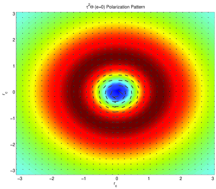
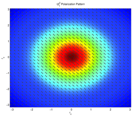
Figure 1: SZ polarization patterns of the double scattering $\tau^{2}\Theta$ ($e=0$, $x>x_{0}$) and $\tau\beta_{t}^{2}$ (cluster moving south-west to north-east) effects.

The CMB appears anisotropic in the frame of a non-radially moving cluster; scattering by IC electrons then polarizes it. Two polarization components are induced; the first is linear in the cluster velocity component transverse to the los, $v_{t}\equiv\beta_{t}c$, but quadratic in $\tau$; the second is linear in $\tau$ but quadratic in $\beta_{t}$. The spatial patterns of the various polarization components can be readily determined when the gas distribution is spehrically symmetric. The polarization patterns arising from scattering off thermal electrons are isotropic in a spherical cluster (Figure 1, left panel) while the corresponding patterns of the kinematic components are clearly anisotropic due to the asymmetry introduced by the direction of the cluster motion (Figure 1, right panel). More realistic gas distributions, substructure and high internal velocities result in complicated polarization patterns (Lavaux, Diego, Mathis & Silk 2004, Shimon, Rephaeli, O’Shea & Norman 2006).

2.1.1 The $\tau^{2}\beta_{t}$ and $\tau\beta_{t}^{2}$ Components

The degree of polarization induced by double scattering in a non-radially moving cluster was determined by Sunyaev & Zeldovich (1980) in the simple case of uniform gas density,

$$P=\frac{1}{40}\tau^{2}\beta_{t}.$$ (7)

This polarization component is frequency-independent in equivalent temperature units since it is a first order Doppler shift. A more complete calculation of this and the other polarization components was formulated by Sazonov & Sunyaev (1999). Viewed along a direction $\hat{\bf{n}}=(\theta,\phi)$, the temperature anisotropy at a point $(X,Y,Z)$, $\Delta T(X,Y,Z,\theta,\phi)$, leads to polarization upon second scattering. The Stokes parameters are calculated from Equation (4),

$$Q(X,Y)\pm iU(X,Y) = \frac{3\sigma_{T}}{16\pi}\int dZn_{e}(X,Y,Z)\int d\Omega\sin^{2}(\theta)e^{\pm 2\phi}\Delta T(X,Y,Z,\theta,\phi)$$ (8)

$$= \frac{3\sigma_{T}}{4\pi}\int dZn_{e}(X,Y,Z)\int d\Omega Y_{2}^{\pm 2}(\theta,\phi)\Delta T(X,Y,Z,\theta,\phi)$$

$Y_{2}^{\pm 2}$ are the $l=2$ and $m=\pm 2$ spherical harmonics. The temperature change resulting from first scatterings is

$$\frac{\Delta T(X,Y,Z,\theta,\phi)}{T}=\sigma_{T}\int d\vec{l}(X^{\prime},Y^{\prime},Z^{\prime},\theta,\phi)n_{e}(X^{\prime},Y^{\prime},Z^{\prime},\theta,\phi)\hat{n}\cdot\beta(X^{\prime},Y^{\prime},Z^{\prime}),$$ (9)

and the optical depth through the point $(X,Y,Z)$ in the direction $(\theta,\phi)$ is

$$\tau(X,Y,Z,\theta,\phi)=\sigma_{T}\int n_{e}(X^{\prime},Y^{\prime},Z^{\prime})d\vec{l}(X^{\prime},Y^{\prime},Z^{\prime},\theta,\phi).$$ (10)

$Q(X,Y)$ and $U(X,Y)$ fully describe the linear 2D polarization field.

To study the polarization profile we define the following polar coordinates

$$X = r\cos\psi$$

$$Y = r\sin\psi$$ (11)

where $r$ is the radial distance from the cluster center. A photon travels a distance ${\bf l}$ before scattering

$$X^{\prime}-X = l\sin\theta\cos\phi$$

$$Y^{\prime}-Y = l\sin\theta\sin\phi$$

$$Z^{\prime}-Z = l\cos\theta.$$ (12)

In these coordinates

$$\frac{\Delta T(X,Y,Z,\theta,\phi)}{T}=\sigma_{T}\int dl(X^{\prime},Y^{\prime},Z^{\prime},\theta,\phi)n_{e}(X^{\prime},Y^{\prime},Z^{\prime},\theta,\phi)\beta(X^{\prime},Y^{\prime},Z^{\prime}).$$ (13)

Assuming the gas velocity is constant (i.e., internal bulk velocities are relatively low) and that the gas density has the familiar $\beta$ profile with index $\beta=2/3$, such that the electron density is $n(r)=n_{0}/(1+r^{2})$, where the radial distance from the center is now taken to be in units of the core radius, $r_{c}$, we obtain

$$\frac{\Delta T(X,Y,Z,\theta,\phi)}{T}=\sigma_{T}n_{0}r_{c}\int_{l=0}^{\infty}\frac{dl}{1+[r^{2}+z^{2}+2l(r\sin\theta\cos(\psi-\phi)+z\cos\theta)+l^{2}]}$$ (14)

where both $l$, and $z$ are given in units of $r_{c}$. Writing

$$A^{2}\equiv 1+r^{2}+z_{0}^{2}$$

$$B\equiv r\sin\theta\cos(\psi-\phi)+z\cos\theta$$ (15)

and integrating over $l$ yields

$$\frac{\Delta T(X,Y,Z,\theta,\phi)}{T}=\sigma_{T}n_{e}^{0}r_{c}\beta\left[\frac{\pi}{2}-\tan^{-1}\left(\frac{B}{\sqrt{A^{2}-B^{2}}}\right)\right]/\sqrt{A^{2}-B^{2}}.$$ (16)

Inserting this into Eq.(8) and carrying out the 3D numerical integration over $z$, $\theta$ and $\phi$ we obtain $Q$ and $U$ as functions of $r$ and $\psi$ only. The total polarization is then obtained from Eq.(6) $P=\sqrt{Q^{2}+U^{2}}$, and by virtue of the fact that $P$ is a scalar quantity, independent of $\psi$. By fitting $P(r)$ over a large range of values $r$ (e.g. $0<\frac{r}{r_{c}}<10$) we obtain the following simple expression

$$P(r)=\frac{3}{16\pi}(n_{e}^{0}\sigma_{T}r_{c})^{2}\beta\left(\frac{ar}{1+br+cr^{2}}\right)$$ (17)

where the constants $a$, $b$ and $c$ are obtained by fitting to the numerical 3D integrations described above

$$a = 0.57938006$$

$$b = -0.85163944$$

$$c = 0.58122608.$$ (18)

The second kinematic polarization component is $\propto\tau\beta_{t}^{2}$; this component is generated by virtue of the fact that the radiation appears anisotropic in the electron frame if the electron motion has a nonvanishing transversal component. From the definition of the Stokes parameters Eq.(4) and the fact that the Doppler effect depends on the angle between the photon direction and the velocity vector, and by choosing the $Z$ axis to coincide with the direction of the electron velocity, one obtains (Chandrasekhar 1950).

$$\frac{d\sigma}{d\Omega}=\frac{3\sigma_{T}}{8}\left(1-\mu_{0}^{2}\right)P_{2}(\mu^{\prime}_{0})\,,$$ (19)

where $P_{2}(\mu^{\prime}_{0})$ is the second Legendre polynomial, the expression for the $Q$ parameter of the scattered radiation is

$$Q(\mu)=\frac{3}{8}\tau(1-\mu_{0}^{2})\int_{-1}^{1}P_{2}(\mu^{\prime}_{0})I(\mu^{\prime}_{0})d\mu^{\prime}_{0}\,.$$ (20)

Here, $\mu^{\prime}_{0}=\cos\theta^{\prime}_{0}$, $\mu_{0}=\cos\theta_{0}$, are the cosines of the angles between the electron velocity and the incoming and outgoing photons, respectively. Expanding the apparent angular distribution of the radiation in Legendre polynomials, and keeping terms up to $\beta^{2}$, the quadrupole moment is determined. The polarization of the singly scattered radiation is then calculated (Sazonov & Sunyaev 1999) by using Equation (4). The level of this polarization component (Sunyaev & Zeldovich 1980) is

$$Q=\frac{x^{2}e^{x}(e^{x}+1)}{20(e^{x}-1)^{2}}\tau\beta_{t}^{2}.$$ (21)

In our chosen frame of reference the Stokes parameter $U$ vanishes due to azimuthal symmetry. Therefore, the total polarization amplitude, $P$, is equal to $Q$ and the polarization is orthogonal to $\beta_{t}$. Relativistic corrections (to the non-relativistic expression of Sunyaev & Zeldovich 1980) were calculated by Challinor, Ford & Lasenby (2000) and Itoh, Nozawa & Kohyama (2000). These corrections generally amount to a $\sim 10\%$ reduction in the value of Q, and are therefore neglected in our calculations.

2.1.2 The $\tau^{2}\Theta$ Component

Analogous to the $\tau^{2}\beta$ component discussed above, double scattering off electrons moving with random thermal velocities can induce polarization that is proportional to $\tau^{2}\Theta$. The anisotropy introduced by single scattering is the thermal component of the SZ effect with temperature change $\Delta T_{t}$. Its dependence on frequency is contained in the following analytic approximation to the exact relativistic calculation (Itoh, Kohyama & Nozawa 1998, Shimon & Rephaeli 2004)

$$\frac{\Delta T(X,Y,Z,\theta,\phi)}{T}=\sigma_{T}\sum_{i=1}^{5}F_{i}(x)\int n_{e}({\bf r})\Theta({\bf r})^{i}dl.$$ (22)

In Equation (22) the integration is along the photon trajectory prior to the second scattering, $F_{i}(x)$ are spectral functions of $x$ (Shimon & Rephaeli 2004). The polarization is obtained by inserting this expression in Eq.(8) and repeating the procedure described in section (2.1.1).

The polarization patterns of these two effects are illustrated in Sunyaev & Zeldovich (1980) and Sazonov & Sunyaev (1999); as can be seen from Figure 1, the polarization due to double scattering on the thermal plasma is expected to vanish when averaged over a beam due to its circular or radial symmetry. When high resoultion, sub-arcminute experiments will be operational the effect will be measured, if sensitivity reaches the few nK level and foreground removal and systematics can be controlled at the required level.

While typical clusters are not perfectly spherical and some residual signal will survive the beam convolution, this signal is expected to be very weak; only second order in the cluster ellipticity $O(e^{2})$. Typically, the correction due to ellipcity is comparable to or smaller than few percent.

2.2 Polarization of Anisotropic Incident Radiation

The large scale anisotropy of the CMB includes a cosmological quadrupole moment at the level of $\approx 15\mu K$, as measured by the all-sky surveys of COBE and WMAP. Knowing that the probability for generating polarization by scattering in clusters is a fraction $\sim\frac{\tau}{10}$ of the incident quadrupole, and that $\tau\sim 0.01$, we expect the resulting polarization signal to be $\approx$15 nK, therefore detection would be extremely challenging, even with next generation experiments.

A similar but smaller component results from scattering of the radiation with a quadrupole moment generated by gravitational waves (from tensor perturbations). Its level is likely to be much smaller; the current limit on the tensor-to-scalar ratio is $T/S<0.4$, deduced from analysis of CMB measurements. The upper (95%) confidence limit from WMAP alone is $0.43$ (Dunkley et al. 2008) and $0.22$, if the analysis includes also SN and BAO (Komatsu et al. 2008). We describe the polarization induced by the primordial quadrupole (both scalar and tensor contributions) below. The main difference between the two is that while density waves do grow during cosmic evolution, tensor perturbations do not, and since we sum the contributions from the entire population of clusters, the redshift evolution of the population has to be known reasonably accurately.

2.2.1 Scalar Contribution

The global quadrupole moment is imprinted on the CMB by the Sachs-Wolfe (SW) effect at the surface of last scattering, and is further boosted by the evolving gravitational fields of density inhomogeneities - the integrated Sachs-Wolfe (ISW) effect. There is no ISW contribution in a purely matter dominated universe, but around recombination the expansion was still partially driven by the residual radiation (which constituted about 1% of the energy budget), and more recently (at $z<0.3$) the expansion became dominated by dark energy, which again caused decay of the gravitational potential. Scattering by IC electrons polarizes the radiation at a level proportional to the product of the rms of the primary quadrupole moment and the cluster scattering optical depth (Sazonov & Sunyaev 1999). Using the WMAP normalization of the CMB quadrupole moment (Bennett  et al.  2003), the maximal polarized signal is expected to be $\simeq 2.6\tau\,\mu K$, and its all-sky average is $\sim 60\%$ of this value (Sazonov & Sunyaev 1999).

It has been noted that the dependence of this polarization component on the CMB quadrupole moment could possibly be used to reduce cosmic variance (Kamionkowski & Loeb 1997), but this seems doubtful (Portsmouth 2004). Another suggestion is that the dependence can probe dark energy models through the redshift evolution of the quadrupole. We note that the polarization induced by the CMB quadrupole can be distinguished from other cluster-induced polarization components by virtue of its large-scale distribution, reflecting that of the primary CMB quadrupole (e.g Baumann & Cooray 2003), and the fact that it is independent of frequency (when expressed in temperature units). The usually quoted value of the quadrupole moment $Q_{rms}\approx 15\mu K$, refers to the primordial quadrupole (generated at recombination) but this quadrupole is directly affected by the evolving gravitational potential, and since perturbations in this potential can possibly alter the quadrupole, it has a redshift dependence imprinted by the evolving potentials. For a power law primordial power spectrum of density perturbations $P(k)\propto k^{n}$, the rms value of the quadrupole is (e.g. Hu 2000)

$$Q^{2}_{{\bf rms}}(z) = \frac{5}{48}\delta_{H}^{2}(1+z)^{2}D^{2}(z)\Omega_{m}^{2}(d_{A}H_{0})^{1-n}\Gamma_{{\bf sw}}(n)$$

$$\Gamma_{{\bf sw}}(n) \equiv 3\sqrt{\pi}\frac{\Gamma[(3-n)/2]\Gamma[(3+n)/2]}{\Gamma[(4-n)/2]\Gamma[(9-n)/2]}$$ (23)

where $\delta_{H}=4.2\times 10^{-5}$, the growth function is

$$D(z)=\frac{H(z)}{H_{0}}\int_{z}^{\infty}dz^{\prime}(1+z^{\prime})\left(\frac{H_{0}}{H(z^{\prime})}\right)^{3}/\int_{0}^{\infty}dz^{\prime}(1+z^{\prime})\left(\frac{H_{0}}{H(z^{\prime})}\right)^{3},$$ (24)

and the Hubble function is

$$H(z)/H_{0}=\sqrt{\Omega_{m}(1+z)^{3}+\Omega_{\Lambda}},$$ (25)

(where $H_{0}$ is the present Hubble constant). In the case of a flat power spectrum $\Gamma_{{\bf sw}}(n=1)=1$ where $n$ is the spectral index of scalar metric perturbations, $\Gamma(x)$ is the Gamma function, $\Omega_{m}$ and $\Omega_{\Lambda}$ are the matter and vacuum density today in units of critical density, and $d_{A}$ is the angular diameter distance to redshift z. The polarization level in temperature units is (Sazonov & Sunyaev 1999)

$$P=\frac{\sqrt{6}}{10}\tau Q_{{\bf rms}}^{{\rm scalar}}.$$ (26)

2.2.2 Tensor Contribution

The scalar metric perturbations dominate the temperature anisotropy at least on small scales but there is also an observational upper limit on the tensorial contribution on large scales ($l<100$), as well as theoretically expected upper limits (i.e. the latter is $r<0.3$ for the simplest inflationary models). It is sufficient to gauge this small tensor contribution by the tensor-to-scalar ratio $r\equiv T/S$. The overall normalization should come from observations, and indeed it turns out that the fractional scalar perturbations are of order $\sim 10^{-5}$. Current upper limits from CMB temperature anisotropy experiments should be considered weak upper limits, for if inflation indeed occurred following a phase transition in the grand unification (GUT) era, a much lower value, $r\approx 0.01$, would be expected. It should be noted that, due to lensing of the CMB by the LSS,which peaks at $l\approx 1000$ but still leaks to the angular degree scales (where the primordial tensor perturbations peak) there is a lower limit to the level of tensor-to-scalar ratio ($r\approx 0.001$) which can be inferred even from ideal measurements (with noise-free detectors) of the primordial B-mode. However, inflation could have taken place before or after the GUT era. The ultimate test will be measurements of B-mode polarization, or a direct detection of the stochastic gravitational waves generated during inflation (presently considered extremely unlikely).

As we show below, similar to the polarization induced by the scalar SW and ISW effects, we expect a small polarization signal to be induced by scattering, and since the effect scales as $C_{l}^{P}\propto\tau^{2}C_{2}^{{\rm tensor}}$, and the current upper limit is $r<0.3$, we expect this signal to be at most $\sim 30\%$ of its scalar counterpart. This component contains both E and B modes (due to the nature of gravitational waves) and has the potential to assist in tightening the limits on the amplitude of gravitational waves. Also, as mentioned above, unlike the scalar quadrupole, the quadrupole induced by gravitational waves does not evolve significantly with redshift, i.e. the ISW effect for the tensor modes effectively vanishes. It is sensitive only to the anisotropic component of the energy-momentum tensor, and in fact decays by about 10% due to neutrino streaming on quadrupole scales (Weinberg 2004), which is a small effect, ignored here. This yields $P=\frac{\sqrt{6}}{10}Q_{{\rm rms}}^{{\rm tensor}}$ as in the case of polarization induced by Compton scattering of the scalar quadrupole moment. Again, $Q_{{\rm rms}}^{{\rm tensor}}$ is obtained from $Q_{{\rm rms}}^{{\rm scalar}}$ (Eq. 23) by setting $n\rightarrow n-1$ and the growth function, which depends on redshift, is set to 1, followed by multiplying the resulting power spectrum by $r$, the current upper limit on the tensor-to-scalar ratio.

3 Power spectrum

Although the temperature anisotropy and polarization induced by galaxy clusters are intrinsically non-gaussian and their angular power spectra do not contain all the statistical information, these spectra still provide important information on the level of the anisotropy and its characteristic scales. The angular power spectrum is essentially the projection of the processed 3D power spectrum on the 2D celestial sphere. There are two characteristic angular scales in the problem; the angular size of a cluster and the typical angular correlation angle on the sky between neighboring (sufficiently rich) clusters. The first is typically a few arcminutes and the correlation angle is $\sim 1^{\circ}$ (if only rich clusters are considered) which correspond to $l\approx 2000-3000$ and $l\approx 200$, respectively. Their relative importance depends on the corresponding 3D power spectra which consists of the Poisson and correlation (clustering) terms. The contribution due to correlations is typically an order of magnitude smaller (e.g., Cooray, Baumann & Sigurdson 2005) and is not considered here. The power spectrum of the anisotropy due to the population of clusters is

$$C_{l}=\int\int|\tilde{\xi}(l,M;z)|^{2}\frac{dn(M;z)}{dM}\frac{dV}{dz}dMdz$$ (27)

where $\tilde{\xi}$ is the Fourier transform of the polarization generated in each cluster

$$\tilde{\xi({\bf l})}=\int d^{2}\theta\xi(\theta)e^{i{\bf l}\cdot{\bf\theta}}.$$ (28)

The above integral is over the mass function of clusters, for which the Press-Schechter distribution (or one of its variants) is usually adopted

$$\frac{dn(M;z)}{dM}=-F(\mu)\frac{\rho_{b}}{M\sigma}\frac{d\sigma}{dM},$$ (29)

where

$$F(\mu)=\sqrt{\frac{2}{\pi}}e^{-\frac{\mu^{2}}{2}}\frac{\mu}{\sigma_{R}},$$ (30)

$M(R)\equiv\frac{4\pi}{3}\rho_{b}R^{3}$ and the mass variance is

$$\sigma^{2}(M;z)=D^{2}(z)\int\frac{dk}{k}\frac{k^{3}P(k)}{2\pi^{2}}|W(kR)|^{2}.$$ (31)

Here $\mu\equiv\delta_{c}(z)/\sigma(z)$ is the critical overdensity for collapse in terms of the mass variance at redshift $z$, and $\rho_{b}$ is the background density at $z=0$, and $W(q)=\frac{3}{q^{3}}[\sin(q)-q\cos(q)]$ is a top-hat window function. The processed density fluctuation power spectrum $P(k)\equiv Ak^{n}T^{2}(k)$ is given in terms of the transfer function $T(k)$ (which is specified below). The normalization constant is determined in terms of the observationally deduced value of $\sigma_{8}$, the mass variance on a scale of $8h^{-1}$ Mpc.

The mass variance evolution with redshift is given by

$$\sigma(M;z)=\frac{g[\Omega_{m}(z)]}{g[\Omega_{m}(0)]}\frac{\sigma(M;0)}{1+z}$$ (32)

where

$$\Omega_{m}(z)=\Omega_{m}(0)(1+z)^{3}.$$ (33)

For the function $g[\Omega_{m}(z)]$ we use the approximate expression (Carroll, Press & Turner 1992)

$$g[\Omega_{m}(z)]=\frac{2.5\Omega_{m}(z)}{\Omega_{m}(z)^{4/7}-\Omega_{\Lambda}+(1+\Omega_{m}(z)/2)(1+\Omega_{\Lambda}/70)}.$$ (34)

We adopt the standard CDM transfer function

$$T(k)=\frac{\ln(1+2.34q)}{2.34q}[1+3.89q+(16.1q)^{2}+(5.46q)^{3}+(6.71q)^{4}]^{-1/4}$$ (35)

with $q\equiv k/(\Omega_{m}h^{2})Mpc^{-1}$ (Bardeen et al. 1986).

The virial relation is used for the gas temperature is obtained assuming virialization

$$kT_{e}=\frac{GM\mu_{H}m_{p}}{3\beta r_{c}(M;z)}$$ (36)

where the core-radius is obtained from the spherical collapse model

$$r_{c}(M;z)=\frac{r_{0}}{1+z}\left[\frac{M}{M_{\sun}}\frac{18\pi^{2}}{\delta_{c}}\frac{\Omega_{m}(z)}{\Omega_{m}(0)}\right]^{1/3}$$ (37)

with $r_{0}=1.69\ {\rm Mpc}/(hp)$ where $p$ is the ratio between the virial to core radius $R_{v}/r_{c}$ (taken here to be 10). The distribution of cluster bulk velocities is derived from the continuity equation

$$v_{{\rm rms}}^{2}=\int\frac{dk}{2\pi}P(k).$$ (38)

The calculation of $\xi({\bf l})$ is significantly simplified by focusing on the total polarization which unlike $Q$ and $U$ - is a scalar field (i.e. a function of r only, as in Eq. 17 or the 2D-projected $\beta$-profile), and - as in the case of temperature anisotropy - we can employ the expansion of scalar-valued 2D plane wave in cylindrical Bessel functions

$$e^{i{\bf l}\cdot\theta}=\sum_{l}i^{l}J_{l}(l\theta)e^{i(\phi-\phi_{l})}$$ (39)

to obtain

$$\tilde{\xi}({\bf l})=2\pi\int\theta d\theta J_{0}(l\theta)\xi(\theta)$$ (40)

where $\xi(\theta)$ is the total polarization. Also, use of a $\beta$-profile for the density implies $\xi(\theta)=\xi(\theta/\theta_{c})$, with $\theta_{c}$ having explicit $M$ and $z$ dependence $\theta_{c}=\theta_{c}(M;z)$ through the spherical collapse model. Now the mass and the radius are related through the density which is fixed to be $18\pi^{2}\rho_{b}(z)$, where $\rho_{b}$ is the background density following the simple spherical collapse model. This density depends on the redshift and therefore the electron density depends on $r$, $M$ and $z$.

To obtain $\xi(\theta)$ we simply take the square root of $Q$ and $U$ added in quadrature at an angular distance $\theta=r/d_{A}$ from the cluster, where $r$ and $d_{A}$ are the physical distance from the cluster center ($r=\sqrt{X^{2}+Y^{2}}$), and the angular diameter distance to the cluster, respectively.

4 Results

All power spectra presented in this work were calculated assuming the $\Lambda$CDM with the WMAP5 best-fit parameters (Komatsu et al. 2008): baryon, dark matter and dark energy densities (in units of the critical density) $\Omega_{b}h^{2}=0.0227$, $\Omega_{c}h^{2}=0.1099$, $\Omega_{\Lambda}=0.742$, respectively, and scalar spectral index, Hubble constant in units of 100 km/sec/Mpc $n_{s}=0.963$, $h=0.72$, respectively. The mass variance parameter is $\sigma_{8}=0.8$.

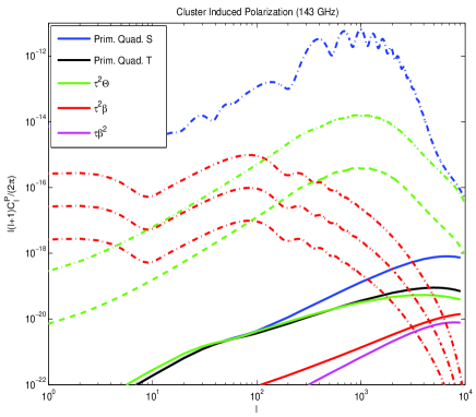
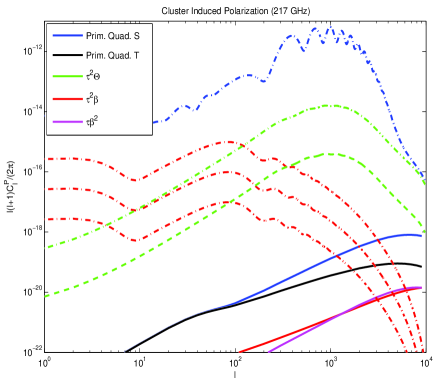
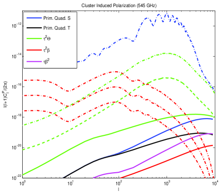
Figure 2: SZ polarization at Planck HFI frequencies: Dot-dashed red lines are the B-modes from the primordial tensor perturbations with tensor-to-scalar-ratios $r=0.1$, $0.01$ and $0.001$ respectively. Dot-dashed blue curve is the E-mode polarization. Dot-dashed green curve is the B-mode from lensing conversion of the E-mode by the LSS. Assuming that this signal can be cleaned to 1 part in 40 we plot the residual B-mode from lensing (dashed green curve). Also shown are five SZ (total-) polarization signals: primordial scalar quadrupole (blue), upper limit (r=0.3) for the effect due to primordial tensor quadrupole (black), $\tau^{2}\Theta$ (green), $\tau^{2}\beta$ (red) and $\tau\beta^{2}$ (magenta).

Power spectra of the cluster polarization components are shown in Fig. 2 together with the corresponding ones of the primary anisotropy. The largest CMB polarized power is the primary E-mode polarization shown by the dot-dashed blue line in Fig. 2. Lensing of this E-mode anisotropy by the LSS produces B-mode pattern (dot-dashed green line in Figure 2) on a level which severely contaminates the primordial B-mode signal from inflation, shown by the dot-dash red lines in Figure 2 for three values of the tensor-to-scalar ratio $r$. As of yet the only information we have on $r$, which determines the amplitude of the B-mode from primordial gravitational waves, is an upper bound of $r<0.3$. Various techniques have been devised to remove the contamination due to the LSS from the primordial signal to allow the determination of the energy scale of inflation (e.g. Hu & Okamoto 2002). However, below $r\approx 0.001$, the residual lensing still dominates the B-mode power even after the lensing contribution is optimally reduced by a projected factor of $\sim 40$, as demonstarated by the dashed green curve in Figure 2. Furthermore, for $r\leq 0.01$ the detection of the primordial B-mode is unlikely due to foreground contamination. Accordingly, the gravitational wave signals for $r=0.1$, $r=0.01$ and $r=0.001$ are shown for comparison.

Our results for the total polarization power spectra induced by scattering in clusters are shown by the solid lines in Fig. 2. Both the polarization due to scattering of the primordial quadrupole (scalar and tensor), the $\tau^{2}\beta_{T}$ effect, and the E/B conversion are independent of frequency, and thus are spectrally indistinguishable from the primordial signal. Separation between these contributions can possibly be based on their different statistical properties (e.g. the characteristic polarization pattern of the former, and non-gaussianity in the later case). Clearly, the largest B-mode signal comes from the E/B mixing by lensing. The $\tau\beta_{T}^{2}$ and the $\tau^{2}\Theta$ components do depend on frequency (as discussed in the previous section) and can be removed from the primary CMB signals by multifrequency observations.

All our results are based on the $\Lambda$CDM with WMAP5 parameters. However, since the SZ effect is a sensitive function of matter clustering, $\sigma_{8}$, and since high-resolution CMB experiments, such as BIMA, CBI and ACBAR, which are sensitive to cluster angular scales infer higher $\sigma_{8}$ than the WMAP5 value of $\simeq 0.82$. With $\sigma_{8}=0.9$, as suggested by galaxy surveys, the cluster polarization power levels are higher by a factor of at least $\sim 2$ (see e.g. Sadeh, Rephaeli & Silk 2007). Polarization from the tensorial quadrupole (black solid line in Fig. 2) is only an upper bound corresponding to $r=0.3$ (close to the current upper limit $0.22$).

5 Discussion

All cluster components calculated here are sub- to few nK and are smaller than the B-mode signal from lensing by $3-4$ orders of magnitude, too weak to have any noticeable impact on parameter estimation, even those which depend on the large scale structure, e.g. neutrino mass $M_{\nu}$, dark energy equation of state, $w$, etc. However, assuming that the lensing signal can be removed to 1 part in 40 by invoking optimal filters based on higher order statistics, cluster signals could potentially contaminate the residual lensing-induced B-modes signal on the few-percent level, again - too weak to have an impact on inflationary models.

Polarization signals from individual rich clusters may be detectable. While these signals may be negligible when averaged out on the full sky, current ground-based endeavors to detect the B-mode polarization typically target only few percent of the sky. Although these ‘radio-quiet’ patches are optimally chosen to minimize the noise, it is not entirely excluded that CMB polarization by individual clusters will have an overall effect of more than the conservative few percent residual contamination shown in Figure 2. Also, it is important to reiterate here that the method of Hu & Okamoto, mentioned above in the context of delensing the sky from the LSS-induced B-mode, indeed rests on the assumption that the unlensed signal is gaussian and that the expected small level of non-gaussianity is due to lensing by the LSS. Therefore, it cannot be employed to remove the non-gaussian SZ polarization from clusters (which indeed was not calculated in this work). This will require, in principle, a customization of similar spatial-filtering methods to the case of galaxy clusters; a problem we have not addressed in this work, mainly because it is expected to be negligibly small for polarization.

The morphology of IC gas typically shows a finite level of ellipticity. It is of interest to assess the implications of a small level of ellipticity on the small-scale power spectrum of the $\tau^{2}\Theta$ polarization component. As Figure 1 illustrates, the effect of double scattering by IC gas in a spherically symmetric cluster will result in vanishing polarization at the cluster center, due to the fact that no quadrupole is generated there from the first scattering. As a result, the $\tau^{2}\Theta$ component drops on very large $l$. However, cluster ellipticity changes this behavior because first scattering of photons travelling along the major and minor axes will result in a few percent quadrupolar change in their corresponding SZ-temperatures, and upon second scattering this small quadrupole will be polarized even at the cluster center. The leading order correction to the $\tau^{2}\Theta$ power spectrum will be $O(e^{2})$, rather than $O(e)$ (since both positive and negative ellipticity statistically avergae out to $\langle e\rangle=0$). In addition, the main qualitative effect will be to boost power at the cluster center as explained above, but this will probably be beyond the reach of even the highest resolution next generation experiments.

Acknowledments

We acknowledge using CAMB to calculate the primordial power spectra. BK gratefully acknowledges support from NSF PECASE Award AST-0548262.

References

- (1) Audit, E., & Simmons, J. F. L. 1999, MNRAS, 305, L27
- (2) Baumann, D., & Cooray, A. 2003, New Astronomy Review, 47, 839
- (3) Bardeen, J. M., Bond, J. R., Kaiser, N., & Szalay, A. S. 1986, ApJ, 304, 15
- (4) Bennett, C., et al. 2003, ApJS, 148, 1
- (5) Carroll, S. M., Press, W. H., & Turner, E. L. 1992, ARAA, 30, 499
- (6) Challinor, A. D., Ford, M. T., & Lasenby, A. N. 2000, MNRAS, 312, 159
- (7) Chandrasekhar, S. 1950, Oxford, Clarendon Press, 1950
- (8) Cooray, A., Melchiorri, A., Silk J. astro – ph/0205214
- (9) Cooray, A., Baumann, D., & Sigurdson, K. 2005, Background Microwave Radiation and Intracluster Cosmology, 309
- (10) Dunkley, J., et al. 2008, arXiv:0803.0586
- (11) Gibilisco, M. 1997, Ap & SS, 249, 189
- (12) Hinshaw, G., et al. 2008, arXiv:0803.0732
- (13) Hu, W. 2000, ApJ, 529, 12
- (14) Hu, W., & Okamoto, T. 2002, ApJ, 574, 566
- (15) Hu, W., DeDeo, S., & Vale, C. 2007, ArXiv Astrophysics e-prints, arXiv:astro-ph/0701276
- (16) Itoh, N., Kohyama, Y., & Nozawa, S. 1998, ApJ, 502, 7
- (17) Itoh, N., Nozawa, S., & Kohyama, Y. 2000, ApJ, 533, 588
- (18) Kamionkowski, M. & Loeb, A. 1997, PRD, 56, 4511
- (19) Komatsu, E., & Kitayama, T. 1999, ApJL, 526, L1
- (20) Komatsu, E., et al. 2008, arXiv:0803.0547
- (21) Lavaux, G., Diego, J. M., Mathis, H., & Silk, J. 2004, MNRAS, 347, 729
- (22) Lewis, A., & King, L. 2006, PRD, 73, 063006
- (23) Ohno, H., Takada, M., Dolag, K., Bartelmann, M., & Sugiyama, N. 2003, ApJ, 584, 599
- (24) Portsmouth, J. 2004, PRD, 70, 063504
- (25) Sadeh, S., Rephaeli, Y., & Silk, J. 2007, MNRAS, 380, 637
- (26) Sazonov, S. Y. & Sunyaev, R. A. 1999, MNRAS, 310, 765
- (27) Seljak, U., & Zaldarriaga, M. 2000, ApJ, 538, 57
- (28) Shimon, M., & Rephaeli, Y. 2004, New Astronomy, 9, 69
- (29) Shimon, M., Rephaeli, Y., O’Shea, B. W., & Norman, M. L. 2006, MNRAS, 368, 511
- (30) Silk, J. 1968, ApJ, 151, 459
- (31) Sunyaev, R. A. & Zeldovich, I. B. 1972, Comm. Ap. Sp. Phys., 4, 173
- (32) Sunyaev, R. A. & Zeldovich, I. B. 1980, MNRAS, 190, 413
- (33) Weinberg, S. 2004, PRD, 69, 023503
- (34) Zaldarriaga, M., & Seljak, U. 1998, PRD, 58, 023003
- (35) Zaldarriaga, M. 2001, PRD, 64, 103001