Persistent current of Luttinger liquid in one-dimensional ring with weak link: Continuous model studied by configuration interaction and quantum Monte Carlo

Abstract

We study the persistent current of correlated spinless electrons in a continuous one-dimensional ring with a single weak link. We include correlations by solving the many-body Schrodinger equation for several tens of electrons interacting via the short-ranged pair interaction $V(x-x^{\prime})$. We solve this many-body problem by advanced configuration-interaction (CI) and diffusion Monte Carlo (DMC) methods which rely neither on the renormalisation group techniques nor on the Bosonisation technique of the Luttinger-liquid model. Our CI and DMC results show, that the persistent current ($I$) as a function of the ring length ($L$) exhibits for large $L$ the power law typical of the Luttinger liquid, $I\propto L^{-1-\alpha}$, where the power $\alpha$ depends only on the electron-electron (e-e) interaction. For strong e-e interaction the previous theories predicted for $\alpha$ the formula $\alpha={(1+2\alpha_{RG})}^{1/2}-1$, where $\alpha_{RG}=[V(0)-V(2k_{F})]/2\pi\hbar v_{F}$ is the renormalisation-group result for weakly interacting electrons, with $V(q)$ being the Fourier transform of $V(x-x^{\prime})$. Our numerical data show that this theoretical result holds in the continuous model only if the range of $V(x-x^{\prime})$ is small (roughly $d\lesssim 1/2k_{F}$, more precisely $4d^{2}k_{F}^{2}\ll 1$). For strong e-e interaction ($\alpha_{RG}\gtrsim 0.3$) our CI data show the power law $I\propto L^{-1-\alpha}$ already for rings with only ten electrons, i.e., ten electrons are already enough to behave like the Luttinger liquid. The DMC data for $\alpha_{RG}\gtrsim 0.3$ are damaged by the so-called fixed-phase approximation. Finally, we also treat the e-e interaction in the Hartree-Fock approximation. We find the exponentially decaying $I(L)$ instead of the power law, however, the slope of $\log(I(L))$ still depends solely on the parameter $\alpha_{RG}$ as long as the range of $V(x-x^{\prime})$ approaches zero.

I Introduction

A clean one-dimensional (1D) wire biased by contacts with negligible backscattering is known to exhibit the conductance quantized as an integer multiple of $e^{2}/h$. The effect can be explained in a Fermi-liquid model of non-interacting quasi-particles. Imry-book ; Davies-98 In fact, a clean 1D system is not a Fermi liquid due to the electron-electron (e-e) interaction. Away from the charge-density-wave instability, the system is a correlated Luttinger liquid with collective bosonic elementary excitations which contrast with independent fermionic quasi-particles of ordinary Fermi liquids Voit . Nevertheless, the Luttinger-liquid model gives for a clean 1D wire the same conductance ($e^{2}/h$ per spin) as the Fermi-liquid model Maslov .

If a localized scatterer is introduced into the wire, the conductance quantization breaks down. For non-interacting electrons, the Landauer formula Imry-book ; Davies-98 expresses the conductance per spin as $(e^{2}/h)|t_{k_{F}}|^{2}$, where $t_{k_{F}}$ is the transmission amplitude through the scatterer at the Fermi level.

In the Luttinger liquid model Kane ; Furusaki , the infinite wire which contains a single structureless scatterer, exhibits the conductance varying with temperature as $\propto T^{2\alpha}$, where $\alpha$ depends only on the e-e interaction. Thus, for $\alpha>0$ (repulsive e-e interaction) the wire is impenetrable at $T\rightarrow 0$ regardless the strength of the scatterer. A similar power law exhibits at $T\rightarrow 0$ the differential conductance as a function of the bias voltage ($\propto U^{2\alpha}$) and conductance versus the wire length ($\propto L^{-2\alpha}$). These power laws are a sign of the Luttinger liquid Kane ; Furusaki ; Dekker . The $T^{2\alpha}$ and $U^{2\alpha}$ laws were successfully measured Dekker .

In this work we deal with similar power laws exhibited by interacting electrons in an isolated mesoscopic 1D ring. In particular, magnetic flux $\phi$ piercing the opening of the mesoscopic ring gives rise to the persistent electron current circulating along the ring Imry-book . This persistent current is given at $T=0$K as $I=-\partial E_{0}(\phi)/\partial\phi$, where $E_{0}$ is the energy of the many-body groundstate. If the ring is clean and the single-particle dispersion law is parabolic, the e-e interaction does not affect the persistent current due to the Galilean invariance of the system Shick .

However, if a single scatterer is introduced, the non-interacting and interacting result differ fundamentally. For non-interacting spinless electrons in the 1D ring containing a single scatterer with transmission probability $|\tilde{t}_{k_{F}}|^{2}\ll 1$, the persistent current at $T=0$K depends on the magnetic flux and ring length ($L$) as Gogolin

$$I=(ev_{F}/2L)\ |\tilde{t}_{k_{F}}|\ \sin(2\pi\phi/\phi_{0}),$$ (1)

where $\phi_{0}=h/e$ is the flux quantum, $k_{F}$ is the Fermi wave vector, and $v_{F}$ is the Fermi velocity. For a spinless Luttinger liquid the persistent current follows the power law $I\propto L^{-\alpha-1}$. More precisely, Gogolin

$$I\propto L^{-\alpha-1}\sin(2\pi\phi/\phi_{0}),$$ (2)

where the power $\alpha$ depends only on the e-e interaction, not on the properties of the scatterer. The formulae (1) and (2) were derived Gogolin assuming large $L$.

The formula (2) can also be obtained heuristically Gogolin as follows. Matveev et al. Matveev analyzed, how the e-e interaction renormalizes the bare transmission amplitude $\tilde{t}_{k_{F}}$ of a single scatterer inside the 1D wire with two contacts. They derived the renormalized amplitude $t_{k_{F}}$ by using the renormalization-group (RG) approach suitable for a weakly-interacting electron gas. If the system length ($L$) is large, their result can be expressed in the form

$$t_{k_{F}}\simeq(\tilde{t}_{k_{F}}/|\tilde{r}_{k_{F}}|)(d/L)^{\alpha},\quad\alpha>0,$$ (3)

where $|\tilde{r}_{k_{F}}|^{2}=1-|\tilde{t}_{k_{F}}|^{2}$, $d$ is the spatial range of the e-e interaction $V(x-x^{\prime})$, and the power $\alpha$ is given (for spinless electrons) by the expression

$$\alpha_{RG}=[V(0)-V(2k_{F})]/2\pi\hbar v_{F},$$ (4)

with $V(q)$ being the Fourier transform of $V(x-x^{\prime})$. We note that the formulae (3) and (4) were derived assuming

$$1\ll\ln(l/d)\ll{\alpha_{RG}}^{-1},$$ (5)

where $l$ is a properly chosen scale of the RG theory Matveev . Moreover, $\alpha=\alpha_{RG}$ only for $\alpha_{RG}\ll 1$ (weak e-e interaction). For strong e-e interaction (say $\alpha_{RG}\simeq 0.5$) the theory Voit ; Polyakov predicts the more general result,

$$\alpha={(1+2\alpha_{RG})}^{1/2}-1.$$ (6)

This result is believed Polyakov to hold for any $V(x-x^{\prime})$ with range $d$ which is finite but which can in principle be quite large (in comparison with $1/k_{F}$). Finally, if we replace in equation (1) the bare amplitude $\tilde{t}_{k_{F}}$ by the renormalized amplitude (3), we recover the power law (2), where $\alpha$ is now given by the microscopic formulae (6) and (4).

In the Luttinger-liquid model, the physics of the low-energy excitations is mapped onto an effective field theory using Bosonization Gogolin , where terms expected to be negligible at low energies are omitted. Within this model, the asymptotic dependence (2) was obtained by using the analogy to the problem of quantum coherence in dissipative environment Gogolin . To avoid this analogy as well as Bosonization, in Ref. Meden the persistent current was calculated by solving the 1D lattice model with nearest-neighbor hopping and interaction. Applying numerical RG methods, the formula (2) was confirmed for long chains and strong scatterers. Meden

However, insofar it has not been verified whether the RG formula (4) holds in a microscopic model which does not rely on the RG approach. We present such microscopic many-body model in this work. Dealing with a continuous model, we can vary the range of the e-e interaction in order to test the robustness of the formula (4) against various shapes of $V(x-x^{\prime})$. This point was not addressed in the lattice-model-based studies as the range of the e-e interaction was fixed to the nearest-neighbor-site interaction.

Further, derivations Gogolin ; Matveev of the formulae (2), (3) and (4) rely on the large number of particles limit. Here we directly address the interesting question what is the minimum number of electrons which exhibits the onset of the Luttinger-liquid dependence $I\propto L^{-\alpha-1}$. As we will illustrate, such behavior can be identified from system sizes of the order of ten electron.

We study the persistent current of correlated electrons in a continuous 1D ring containing the strongly-reflecting scatterer, because strong backscattering is known Gogolin ; Matveev ; Meden to reduce the system size necessary to achieve the $L^{-\alpha-1}$ asymptotics. Using advanced configuration-interaction (CI) and diffusion Monte Carlo (DMC) methods, we solve the continuous many-body Schrodinger equation for several tens of electrons interacting via the e-e interaction

$$V(x-x^{\prime})=V_{0}\,\exp(-\left|x-x^{\prime}\right|/d).$$ (7)

Interaction (7) emulates screening (say by the metallic gates) and allows us to compare our results with the results of the correlated models Gogolin ; Matveev ; Meden which also assume the e-e interaction of finite range. Our CI and DMC calculations do not rely on the RG techniques and solve the continuous model, unlike the RG studies focused largely on the lattice models Meden ; Enss-2005 ; Meden-2005 ; Andregassen . Our numerical data show that the formulae (6) and (4) hold only if the range of the e-e interaction is small ($d\lesssim 1/2k_{F}$). For strong e-e interaction ($\alpha_{RG}\gtrsim 0.3$) our CI data show the power law $I\propto L^{-1-\alpha}$ already for rings with only ten electrons. In other words, ten electrons are already sufficient to show the Luttinger-liquid behavior.

It is known that the fermion sign problem causes an exponential inefficiency of the DMC method Foulkes-01 unless it is circumvented by the so-called fixed-node or the fixed-phase approximation for inherently complex wave functions Ortiz . The accuracy of our DMC results for $\alpha_{RG}\gtrsim 0.3$ is therefore limited by the quality of the phase in the Hartree-Fock trial wave function which is employed in the fixed-phase approximation. Since Hartree-Fock is the simplest possible trial wave function and does not capture the Luttinger-liquid correlation effects it is not surprising that the fixed-phase bias becomes pronounced. We analyze these findings later in detail. (Our DMC should not be confused with the path-integral Monte-Carlo methods Fisher-93 ; Egger-93 ; Egger-95 ; Egger-2004 , used to study the tunnelling conductance of the Luttinger liquid in the bosonised model.)

Finally, we treat the e-e interaction in the self-consistent Hartree-Fock calculation. We find for large $L$ the exponentially decaying $I(L)$ instead of the power law. However, the slope of $\log(I(L))$ still depends solely on the parameter $\alpha_{RG}$ given by the RG formula (4), as long as the range of $V(x-x^{\prime})$ approaches zero.

In section II.A we start with the single-particle approach to the 1D ring. In section II.B we define our interacting many-body model. In section II.C we outline how we solve the many-body model in the Hartree-Fock approximation. In sections II.D and II.E we describe how we obtain the fully-correlated many-body solution by means of the DMC method and CI method. Our results are discussed in section III and a summary is given in section IV. Technical details are in the appendices.

II Theory

II.1 Single-particle model

We consider the circular 1D ring threaded by magnetic flux $\phi=BS=AL$, where $S$ is the area of the ring, $B$ is the magnetic field (constant and perpendicular to the ring area), and $A$ is the magnitude of the resulting vector potential (circulating along the ring circumference). In this section we discuss the single-particle states in such ring. In general, the single-electron wave functions $\psi_{n}(x)$ in the 1D ring obey the Schödinger equation

$$\left[\frac{\hbar^{2}}{2m}\left(\frac{1}{i}\frac{\partial}{\partial x}+\frac{2\pi}{L}\frac{\phi}{\phi_{0}}\right)^{2}+U(x)\right]\psi_{n}(x)=\varepsilon_{n}\psi_{n}(x)$$ (8)

with the cyclic boundary condition

$$\psi_{n}(x+L)=\psi_{n}(x)\,,$$ (9)

where $m$ is the electron effective mass, $x$ is the electron coordinate along the ring, and $U(x)$ is an external single-particle potential.

We introduce the wave functions $\varphi_{n}(x)$ by substitution

$$\psi_{n}(x)=\varphi_{n}(x)\exp{\left(-i\frac{2\pi}{L}\frac{\phi}{\phi_{0}}x\right)}\,.$$ (10)

If we set (10) into (8) and (9), we obtain the equation

$$\left[-\frac{\hbar^{2}}{2m}\frac{d^{2}}{dx^{2}}+U(x)\right]\varphi_{n}(x)=\varepsilon_{n}\varphi_{n}(x)$$ (11)

with the boundary condition

$$\varphi_{n}(x+L)=\exp\left(i2\pi\frac{\phi}{\phi_{0}}\right)\varphi_{n}(x)\,.$$ (12)

Equations (11) and (12) can be solved for an arbitrary potential $U(x)$ numerically. Consider first the ring region $x\in\langle-L/2,L/2\rangle$ as a straight-line segment of an infinite 1D wire. Inside the segment the potential is $U(x)$, outside we keep it zero. Therefore, the wave function outside is

$$\varphi_{k}(x)=ae^{ikx}+be^{-ikx}\,,\;x\leq-L/2\,,$$ (13)

$$\varphi_{k}(x)=ce^{ikx}+de^{-ikx}\,,\;x\geq L/2\,.$$ (14)

The amplitudes $a$ and $b$ are related to $c$ and $d$ by

$$\left(\begin{array}[]{c}c\\ d\end{array}\right)=T_{0}\left(\begin{array}[]{c}a\\ b\end{array}\right)\,,$$ (15)

where $T_{0}$ is the transfer matrix Davies-98

$$T_{0}=\left(\begin{array}[]{cc}\frac{1}{t_{k}^{*}}&-\frac{r_{k}^{*}}{t_{k}^{*}}\\ -\frac{r_{k}}{t_{k}}&\frac{1}{t_{k}}\end{array}\right)\,,$$ (16)

with $t_{k}$ and $r_{k}$ being the transmission and reflection amplitudes of the electron impinging the region $\langle-L/2,L/2\rangle$ from the left. At the boundaries we express $\varphi_{k}(-L/2)$ and $\varphi_{k}(L/2)$ by using equations (13) and (14). To come back to the ring threaded by magnetic flux, we relate $\varphi_{k}(-L/2)$ and $\varphi_{k}(L/2)$ through the boundary condition (12). Combining the obtained relation with the equations (15) and (16) we obtain the equation

$$T\left(\begin{array}[]{c}a\\ b\end{array}\right)=\exp(i2\pi\frac{\phi}{\phi_{0}})\left(\begin{array}[]{c}a\\ b\end{array}\right)\,,$$ (17)

where

$$T=\left(\begin{array}[]{cc}\frac{1}{t_{k}^{*}}e^{ikL}&-\frac{r_{k}^{*}}{t_{k}^{*}}e^{ikL}\\ -\frac{r_{k}}{t_{k}}e^{-ikL}&\frac{1}{t_{k}}e^{-ikL}\end{array}\right)\,.$$ (18)

Thus $\exp(i2\pi\phi/\phi_{0})$ is the eigenvalue of the matrix $T$. The product of the eigenvalues of this matrix is given by its determinant which is unity. The second eigenvalue is thus $\exp(-i2\pi\phi/\phi_{0})$. Their sum is equal to the matrix trace Davies-98 , which gives the equation for the spectrum remark1 ,

$$\cos\left(2\pi\frac{\phi}{\phi_{0}}\right)={\rm Re}\left[\frac{\exp(-ikL)}{t_{k}}\right]\,.$$ (19)

The numerical solution of equation (19) has to be combined with numerical computation of the transmission amplitude $t_{k}$ (the algorithm for computation of $t_{k}$ and $r_{k}$ is described in the Appendix A). The solution of equation (19) gives us the dependence $k_{n}(\phi)$ and eventually the single-particle eigenenergy $\varepsilon_{n}(\phi)=\hbar^{2}k_{n}^{2}(\phi)/2m$.

For each $k_{n}(\phi)$ we can also calculate the wave function $\varphi_{n}(x)$. We proceed as follows. By means of equations (17) and (18) we express the amplitude $a$ in the form

$$a=\left[\frac{1}{r_{k_{n}}}-\frac{t_{k_{n}}}{r_{k_{n}}}e^{i(2\pi\phi/\phi_{0}+k_{n}L)}\right]b\,,$$ (20)

where the amplitude $b$ can be obtained by normalizing the wave function. Then we express from equation (13) the boundary conditions $\varphi_{n}(-L/2)$ and $d\varphi_{n}(-L/2)/dx$. Finally, we combine these boundary conditions with numerical solution of equation (11) in the discrete form Press

$$\varphi_{n}\left(x_{j+1}\right)=\\ \left[2+\frac{2m}{\hbar^{2}}\left(U\left(x_{j}\right)-\varepsilon_{n}\right)\Delta^{2}\right]\varphi_{n}\left(x_{j}\right)-\varphi_{n}\left(x_{j-1}\right)\,,$$ (21)

where $\Delta$ is the step, $x_{j}=j\Delta$, and $j=0,\pm 1,\pm 2,\dots$. Once the wave functions $\varphi_{n}(x)$ are known, the wave functions $\psi_{n}(x)$ can be obtained by means of the relation (10).

II.2 Interacting many-body model

We now consider the ring with $N$ interacting 1D electrons. This system is described by the Hamiltonian

$$\hat{H} = \sum\limits_{j=1}^{N}\left[\frac{\hbar^{2}}{2m}\left(\frac{1}{i}\frac{\partial}{\partial x_{j}}+\frac{2\pi}{L}\frac{\phi}{\phi_{0}}\right)^{2}+\gamma\delta(x_{j})\right]$$ (22)

$$+ \frac{1}{2}\sum\limits_{{i,j=1}\atop{i\neq j}}^{N}V(x_{j}-x_{i})\,,$$

where $x_{j}$ is the coordinate of the $j$-th electron, $\gamma\delta(x)$ is the potential of the scatterer, and $V(x_{j}-x_{i})$ is the e-e interaction (7). The eigenfunction $\Psi(x_{1},x_{2},\dots,x_{N})$ and eigenenergy $E$ obey the Schödinger equation

$$\hat{H}\Psi=E\Psi$$ (23)

with the cyclic boundary condition

$$\Psi(x_{1},\dots,x_{i}+L,\dots,x_{N})=\Psi(x_{1},\dots,x_{i},\dots,x_{N})$$ (24)

for $i=1,2,\dots,N$.

If the system is in the groundstate with eigenfunction $\Psi_{0}(x_{1},x_{2},\dots,x_{N})$ and eigenenergy $E_{0}$, the persistent current can be expressed as

$$I=\left<\Psi_{0}\right|\hat{I}\left|\Psi_{0}\right>\,$$ (25)

where

$$\hat{I}=-\frac{e}{mL}\sum\limits_{j=1}^{N}\left(\frac{\hbar}{i}\frac{\partial}{\partial x_{j}}+\frac{e\phi}{L}\right)$$ (26)

is the $N$-particle current operator. One can calculate $I$ directly from the relation (25), or one can rewrite (25) by means of the Hellman-Feynman theorem

$$\frac{\partial E}{\partial\phi}=\left<\Psi_{0}\right|\frac{\partial\hat{H}}{\partial\phi}\left|\Psi_{0}\right>\,.$$ (27)

Using (27), (26), and (22) one gets the formula Imry-book ; Eckern

$$I=-\frac{\partial}{\partial\phi}E_{0}(\phi)\,.$$ (28)

II.3 Hartree-Fock approximation

In the Hartree-Fock model, the ground-state wave function $\Psi_{0}$ is approximated by the Slater determinant

$$\Psi_{0}(x_{1},\dots,x_{N})=\frac{1}{\sqrt{N!}}\left|\begin{array}[]{ccc}\psi_{1}(x_{1})&\cdots&\psi_{1}(x_{N})\\ \vdots&\ddots&\vdots\\ \psi_{N}(x_{1})&\cdots&\psi_{N}(x_{N})\end{array}\right|\,.$$ (29)

The wave functions $\psi_{n}(x)$ obey the Hartree-Fock equation

$$\left[\frac{\hbar^{2}}{2m}\left(-i\frac{\partial}{\partial x}+\frac{2\pi}{L}\frac{\phi}{\phi_{0}}\right)^{2}+\gamma\delta(x)\right.\\ \left.\phantom{\frac{\hbar^{2}}{2m}}+U_{H}(x)+U_{F}(n,x)\right]\psi_{n}(x)=\varepsilon_{n}\psi_{n}(x)$$ (30)

with the boundary condition

$$\psi_{n}(x+L)=\psi_{n}(x)\,,$$ (31)

where

$$U_{H}(x)=\sum_{n^{\prime}}\int dx^{\prime}V(x-x^{\prime})|\psi_{n^{\prime}}(x^{\prime})|^{2}$$ (32)

is the Hartree potential and

$$U_{F}(n,x)=\\ -\frac{1}{\psi_{n}(x)}\sum\limits_{n^{\prime}}\int dx^{\prime}V(x-x^{\prime})\psi_{n}(x^{\prime})\psi_{n^{\prime}}^{*}(x^{\prime})\psi_{n^{\prime}}(x)$$ (33)

is the Fock nonlocal exchange term (expressed as an effective potencial for further convenience). In the equations (32) and (33) we sum over all occupied states $n^{\prime}$.

If we use again the substitution

$$\psi_{n}(x)=\varphi_{n}(x)\exp{\left(-i\frac{2\pi}{L}\frac{\phi}{\phi_{0}}x\right)}\,,$$ (34)

the equations (30)-(33) give the Hartree-Fock equation

$$\left[-\frac{\hbar^{2}}{2m}\frac{d^{2}}{dx^{2}}+\gamma\delta(x)+U_{H}(x)+U_{F}(n,x)\right]\varphi_{n}(x)\\ =\varepsilon_{n}\varphi_{n}(x)$$ (35)

with the boundary condition

$$\varphi_{n}(x+L)=\exp\left(i2\pi\frac{\phi}{\phi_{0}}\right)\varphi_{n}(x)\,,$$ (36)

where the potentials $U_{H}(x)$ and $U_{F}(n,x)$ are still given by equations (32) and (33), but with $\psi_{n}$ replaced by $\varphi_{n}$. From equations (22)-(36) the groundstate energy $E_{0}=\langle\Psi_{0}|H|\Psi_{0}\rangle$ can be expressed as

$$E_{0}=\sum\limits_{n}\left[\varepsilon_{n}-\frac{1}{2}\left\langle\varphi_{n}\left|U_{H}(x)+U_{F}(n,x)\right|\varphi_{n}\right\rangle\right]\,.$$ (37)

The Hartree-Fock equation (35) can be solved by the same procedure as the single-particle equation (11) assuming that the potential $U(x)\equiv\gamma\delta(x)+U_{H}(x)+U_{F}(n,x)$ is known. We apply this procedure iteratively in order to obtain the self-consistent Hartree-Fock solution. In the first iteration step we solve equation (35) for the non-interacting gas, i.e., for $U_{H}(x)=0$ and $U_{F}(n,x)=0$. The resulting $\varphi_{n}(x)$ is used to evaluate the Hartree and Fock potentials, where the term $U_{F}(n,x)$ has to be evaluated for each $n$ separately. These potentials are used in the second iteration step to obtain new $\varphi_{n}(x)$ and new potentials $U_{H}(x)$ and $U_{F}(n,x)$, etc., until the energies $\varepsilon_{n}$ and ground-state energy (37) do not change anymore. In the Appendix B the iteration procedure is described including a few nontrivial details. Setting the resulting ground-state energy (37) into (28) we obtain the persistent current. Of course, this Hartree-Fock calculation does not include the many-body correlations. To include the correlations we use the DMC and CI techniques described in the next two sections.

II.4 Diffusion Monte Carlo (DMC) model

Consider first the $N$-electron 1D Schödinger equation

$$\hat{\mathcal{H}}\Psi(\textbf{X})=E\Psi(\textbf{X})$$ (38)

with Hamiltonian

$$\hat{\mathcal{H}}=-\frac{\hbar^{2}}{2m}\sum_{i=1}^{N}\frac{\partial^{2}}{\partial x_{i}^{2}}+V(X),$$ (39)

where $\textbf{X}=(x_{1},x_{2},\dots,x_{N})$, the potential energy $V(X)$ incorporates all single-electron interactions and all pair electron-electron interactions, and the wave-function $\Psi(\textbf{X})$ is assumed to obey the cyclic condition (24). If $\Psi(\textbf{X})$ is a real function, the DMC method is capable to find the exact ground-state solution of equation (38). We briefly summarize how the DMC works Foulkes-01 .

Instead of directly solving the equation (38), the DMC solves the time-dependent diffusion problem Foulkes-01

$$-\partial\Psi(\textbf{X},t)/\partial t=\left(\hat{\mathcal{H}}-E_{T}\right)\Psi(\textbf{X},t),$$ (40)

where $E_{T}$ is a trial energy. One can write (40) in the integral form Foulkes-01

$$\Psi(\textbf{X},t+\tau)=\int d\textbf{X'}\ G_{\textbf{X}\leftarrow\textbf{X'}}(\tau)\ \Psi(\textbf{X'},t),$$ (41)

where $G_{\textbf{X}\leftarrow\textbf{X'}}(\tau)=\langle\textbf{X}|\exp(-(\hat{\mathcal{H}}-E_{T})\tau)|\textbf{X'}\rangle$ is the Green’s function and $\tau$ is a time step. Equation (41) allows to project the ground state $\Psi_{0}(\textbf{X})$ from any trial wave function $\Psi_{T}(\textbf{X})$ which has a nonzero overlap with $\Psi_{0}(\textbf{X})$. Inserting any trial $\Psi_{T}(\textbf{X})$ and $E_{T}$ into (41) gives

$$\Psi_{T}(\textbf{X},\tau\rightarrow\infty)=\Psi_{0}(\textbf{X})\langle\Psi_{0}|\Psi_{T}\rangle\lim\limits_{\tau\rightarrow\infty}\exp[-\tau(E_{0}-E_{T})].$$ (42)

By adjusting $E_{T}$ to equal $E_{0}$ one can make the exponential factor constant. It is also important that the Green’s function $G_{\textbf{X}\leftarrow\textbf{X'}}(\tau)$ can be expressed Foulkes-01 for $\tau\rightarrow 0$ as

$$G_{X\leftarrow X^{\prime}}(\tau)\approx(2\pi\tau)^{-3N/2}\exp\left[-\frac{(X-X^{\prime})^{2}}{2\tau}\right]\\ \times\exp\left(-\tau\left[V(X)+V(X^{\prime})-2E_{T}\right]/2\right).$$ (43)

In the DMC algorithm the equation (41) is solved stochastically based on the action of the projection operator $\exp[-\tau(\hat{\mathcal{H}}-E_{T})]$ Foulkes-01 . At time $t=0$ one chooses a proper trial wave function $\Psi_{T}(\textbf{X})$. A set of walkers (sampling points in the $N$-dimensional electron configuration space) is generated according to the distribution $\Psi_{T}(\textbf{X})$. A small timestep $\tau$ is chosen. The walkers are propagated from X to X’ according to the kernel $G_{\textbf{X}\leftarrow\textbf{X'}}(\tau)$ in the form (43). In the new sample point X’, the expectation values are calculated and the starting value of $E_{T}$ is adjusted. Eventually, the ground state expectation values are projected and sampled.

The problem is that the wave function $\Psi(\textbf{X})$ obeying the many-body equation (23) is complex because the Hamiltonian (22) contains the magnetic flux. The problem can be partly eliminated by means of the fixed-phase approximation Ortiz . Using

$$\Psi(\textbf{X})=\left|\Psi(\textbf{X})\right|e^{i\Phi(\textbf{X})}$$ (44)

one can split the equation (23) into the real part and imaginary part. The real part reads

$$\hat{H}_{\text{eff}}\left|\Psi(\textbf{X})\right|=E\left|\Psi(\textbf{X})\right|,$$ (45)

where

$$\hat{H}_{\text{eff}}=-\frac{\hbar^{2}}{2m}\sum_{i=1}^{N}\frac{\partial^{2}}{\partial x_{i}^{2}}+\frac{1}{2m}\sum_{i=1}^{N}\left(\hbar\frac{\partial}{\partial x_{i}}\Phi+\frac{e\phi}{L}\right)^{2}$$

$$+\gamma\sum_{i=1}^{N}\delta(x_{i})+\frac{1}{2}\sum\limits_{{i,j=1}\atop{i\neq j}}^{N}V(x_{i}-x_{j}),$$ (46)

and the imaginary part is

$$\sum_{i=1}^{N}\frac{\partial}{\partial x_{i}}\left[|\Psi|^{2}\left(\hbar\frac{\partial}{\partial x_{i}}\Phi+\frac{e\phi}{L}\right)\right]=0.$$ (47)

Equation (45) is the effective Schödinger equation for the modul $\left|\Psi(\textbf{X})\right|$, with the Hamiltonian $\hat{H}_{\text{eff}}$ depending on the phase $\Phi(\textbf{X})$. Since $\left|\Psi(\textbf{X})\right|$ is real and $\hat{H}_{\text{eff}}$ has the same form as (39), the equation (45) can be solved by means of the DMC if the phase $\Phi(\textbf{X})$ is given. In this work we choose the trial wave function $\Psi_{T}(\textbf{X})$ to be equal to the Slater determinant (29) of the self-consistently determined Hartree-Fock ground state and we fix the phase $\Phi(\textbf{X})$ to the phase of this Slater determinant. The DMC thus gives the lowest possible ground-state energy $E_{0}$ within the chosen phase Ortiz . Eventually, we obtain the persistent current from (28) by finite differences evaluated by correlated sampling Filipi . Our preliminary DMC results are briefly discussed in Vagner ; Krcmar .

To go beyond the fixed phase approximation one has to couple the DMC solution of equation (45) with the numerical solution of equation (47). We do not attempt to do so. However, in section III we check the fixed phase approximation by comparing the DMC results with the CI calculations which are free of such approximation.

II.5 Configuration-interaction (CI) model

Before starting with the CI procedure we need to solve the single-electron problem

$$\left[\frac{\hbar^{2}}{2m}\left(\frac{1}{i}\frac{\partial}{\partial x}+\frac{2\pi}{L}\frac{\phi}{\phi_{0}}\right)^{2}+\gamma\delta(x)\right]\psi_{n}(x)=\varepsilon_{n}\psi_{n}(x)$$ (48)

with the cyclic condition $\psi_{n}(x+L)=\psi_{n}(x)$. We do so by using the method described in Section II.A. We obtain the wave functions $\psi_{n}(x)$ and energy levels $\varepsilon_{n}$ not only for the $N$ lowest energy levels but also for the infinite ladder of excited states, of course, with an upper cutoff.

Consider now the non-interacting many-body problem

$$\sum_{j=1}^{N}\left(\frac{\hbar^{2}}{2m}\left(\frac{1}{i}\frac{\partial}{\partial x_{j}}+\frac{2\pi}{L}\frac{\phi}{\phi_{0}}\right)^{2}+\gamma\delta(x_{j})\!\!\right)\chi_{n}(\textbf{X})=\mathcal{E}_{n}\chi_{n}(\textbf{X}),$$ (49)

where $\textbf{X}=(x_{1},x_{2},\dots,x_{N})$. Clearly, the eigenenergies $\mathcal{E}_{n}$ are given as

$$\mathcal{E}_{n}=\varepsilon_{n_{1}}+\dots+\varepsilon_{n_{N}}$$ (50)

and the wave functions $\chi_{n}$ are the Slater determinants

$$\chi_{n}=\frac{1}{\sqrt{N!}}\left|\begin{array}[]{ccc}\psi_{n_{1}}(x_{1})&\dots&\psi_{n_{N}}(x_{1})\\ \vdots&\ddots&\vdots\\ \psi_{n_{1}}(x_{N})&\dots&\psi_{n_{N}}(x_{N})\end{array}\right|,$$ (51)

where the quantum numbers $n_{1},\dots,n_{N}$ label the state of the first, $\dots,N$-th electron, respectively, and the quantum number $n$ labels the many-body state corresponding to the specific set of $N$ occupied single-electron levels $\varepsilon_{n_{1}},\dots,\varepsilon_{n_{N}}$. For instance, the figure 1 depicts creation of all Slater determinants in the three-electron system, when only six lowest single-electron levels are considered.

To solve the interacting many-body problem (23), the CI method Szabo ; Jensen relies on the expansion

$$\Psi=c_{0}\chi_{0}+c_{1}\chi_{1}+c_{2}\chi_{2}+\dots\\ .$$ (52)

Using this expansion and equation $\langle\chi_{n}|\hat{H}|\Psi\rangle=\langle\chi_{n}|E|\Psi\rangle$ we obtain from (23) the infinite set of equations

$$\sum_{j=0}^{\infty}\left(\mathcal{E}_{j}\delta_{nj}+V_{nj}\right)c_{j}=Ec_{n},\quad n=0,1,\dots,\infty,$$ (53)

where

$$V_{nj}=\frac{1}{2}\langle\chi_{n}|\sum\limits_{{k,l=1}\atop{k\neq l}}^{N}V(x_{k}-x_{l})|\chi_{j}\rangle.$$ (54)

We reduce the infinite number of single-energy levels $\varepsilon_{j}$ to the finite one by introducing a proper upper energy cutoff. This reduces the infinite number of equations (53) to a certain finite number $M+1$. We get the finite system

$$\sum_{j=0}^{M}\left(\mathcal{E}_{j}\delta_{nj}+V_{nj}\right)c_{j}=Ec_{n},$$ (55)

where $n=0,1,\dots,M$. This system determines the eigenvalues $E_{l}$ and eigenvectors $(c^{l}_{0},c^{l}_{1},\dots,c^{l}_{M})$ for $l=0,1,\dots,M$. We obtain the groundstate energy $E_{l=0}$ and groundstate wave function $\Psi_{l=0}$ by solving the system with ARPACK, or alternatively with LAPACK. Once $E_{0}$ and $\Psi_{0}$ are known, the persistent current can be obtained from (28) or (25).

The problem of the CI method is, that for $N_{max}$ single-particle levels the expansion (52) still contains $\left({N_{max}}\atop{N}\right)$ Slater determinants. For a reasonably chosen cutoff, the solution of the equations (55) is not feasible already for systems with about ten electrons, as the memory requirements are too large. The question is which determinants have to be kept in the expansion (52) and which can be omitted without damaging the final results. This problem is known in the quantum chemistry Szabo ; Jensen where the CI is applied to calculate the energy spectra of molecules. We cannot apply here directly the tricks from the quantum chemistry because our problem is rather special; we search for the persistent current in the 1D ring pierced by magnetic flux. We prefer the following two approaches.

Figure 1: Schematic sketch of how the determinants $\chi_{n}$ are created for $n=0,1,\dots$ in the three-electron system with the ladder of single-particle levels restricted to six lowest levels. The occupied levels constituting the state $\chi_{n}$ are labelled by circles. In the CI method the many-body state $\Psi$ of the interacting system is expanded as $\Psi=c_{0}\chi_{0}+c_{1}\chi_{1}+c_{2}\chi_{2}+\dots$.

Our first CI approach, below referred as the FCI, conceptually resembles the full CI and can be understood by means of the sketch in the figure 1. After choosing the cutoff for the single-particle energy we add into the expansion (52) first the Slater determinant of the ground state, then all determinants with a single excited electron (the single-excitations), all determinants with two excited electrons (the double-excitations), all determinants with three excited electrons (the triple-excitations), etc. If the results do not change, we cut the expansion by stopping to increase the number of the excited electrons. Some preliminary FCI results are briefly discussed in Krcmar .

Our second CI approach, introduced by two of us in Ref. Indlekofer , is called the bucket-brigade CI method (BBCI). After choosing the cutoff for the single-particle energy, we need to asses importance of the remaining Slater determinants in the expansion (52). In principle, one can compute for each determinant $\chi_{n}$ the energy $\left<\chi_{n}\right|\hat{H}\left|\chi_{n}\right>$, where $\hat{H}$ is the Hamiltonian (22). The obtained numerical values $\left<\chi_{n}\right|\hat{H}\left|\chi_{n}\right>$ can be ordered increasingly and we can assume that this orders the determinants $\chi_{n}$ according to their decreasing importance. We can order the determinants in the expansion (52) according to this importance criterion (a-priori measure of importance) and we can truncate the expansion after reaching convergence of the final results. This is the basic idea of the BBCI method, the term ”bucket brigade” is related to the technical implementation Indlekofer reviewed in the Appendix C.

In the next section, reliability of our importance criterion is supported by a successful convergence of the BBCI results. We cannot prove the criterion exactly, but we can give a simple intuitive motivation. We search for the best minimum of the ground-state energy. Therefore, the larger the energy $\left<\chi_{n}\right|\hat{H}\left|\chi_{n}\right>$ the smaller should be the weight of the given $\chi_{n}$ in the ground-state expansion (52). It is important that the BBCI allows us to treat more electrons than the FCI, as it reduces the expansion (52) more efficiently. Another CI algorithm, more efficient than the FCI, is the CI approach of Ref. Greer, , where the determinants are selected by means of a proper Monte Carlo algorithm.

III Results

III.1 Luttinger-liquid scaling in CI and DMC models

Our calculations are performed for parameters typical of a GaAs ring. We use the electron effective mass $m=0.067m_{0}$ and electron density $n_{e}=N/L=5\times 10^{7}$ m^-1. The strength $V_{0}$ and range $d$ of our e-e interaction (7) are properly varied to demonstrate various e-e interaction effects. In practice, screening by metallic gates can be used to vary $d$ while $V_{0}$ can be varied by varying the (finite) cross-section of the 1D ring. We study the rings containing a strong scatterer with $|\tilde{t}_{k_{F}}|^{2}\ll 1$, because in such case the persistent current reaches asymptotic dependence on $L$ for relatively small $L$. Our conclusions hold for any 1D system, no matter what material is used.

In figure 2 the persistent current $I$ in the GaAs ring with one strong scatterer is calculated as a function of the ring length $L$ for magnetic flux $\phi=0.25\phi_{0}$. The scatterer is the $\delta$ barrier with transmission $|\tilde{t}_{k_{F}}|^{2}=0.03$. The power law $LI\propto L^{-\alpha}$ decays in the log scale linearly with slope $-\alpha$, the same decay show for large $L$ the CI and DMC data. Agreement of the FCI and BBCI data is very good, the DMC data are close to the CI data.

Let us check whether our numerical values of $\alpha$ agree with the formula (6). The Fourier transform of our e-e interaction (7) is $V(q)=2V_{0}d/(1+q^{2}d^{2})$. Using this expression we can write the RG formula (4) in the form

$$\alpha_{RG}=\frac{4V_{0}mk_{F}d^{3}}{\pi\hbar^{2}(1+4{k_{F}}^{2}d^{2})}.$$ (56)

The dashed lines in the figure 2 show the power law $LI\propto L^{-\alpha}$, with $\alpha$ given by the formula (6) and $\alpha_{RG}$ calculated from the formula (56). The proportionality factor (specified later on) causes in the log scale only a vertical shift of the linear law $\log(LI)=-\alpha\log(L)+$const. We thus can conclude that the CI and DMC data in the figure 2 exhibit the $L^{-\alpha}$ decay with the power $\alpha$ in good agreement with the theoretical formulae (6) and (56).

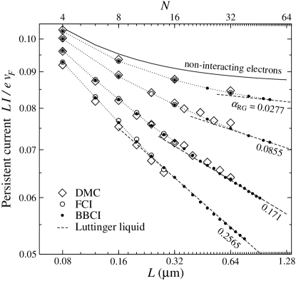
Figure 2: Persistent current $LI/ev_{F}$ versus the ring length $L$ for the GaAs ring with a single scatterer. The transmission of the scatterer is $|\tilde{t}_{k_{F}}|^{2}=0.03$, magnetic flux is $\phi=0.25\phi_{0}$. The upper horizontal axis shows the electron number $N=n_{e}L$, where $n_{e}=5\times 10^{7}$ m^-1. The range of the e-e interaction is fixed to $d=3$nm while the magnitude $V_{0}$ is varied. The full curve is our numerical result for $V_{0}=0$ (non-interacting electrons). This curve saturates for large $L$ exactly at the value $0.5|\tilde{t}_{k_{F}}|$, predicted by the asymptotic formula (1). The symbols show our FCI, BBCI and DMC results for various $V_{0}$ shown in table 1, the dotted lines connecting the BBCI data are a guide for eye. The dashed lines show the Luttinger liquid asymptotics $LI\ \propto L^{-\alpha}$ for $\alpha={(1+2\alpha_{RG})}^{1/2}-1$, where the values of $\alpha_{RG}$ (listed in the figure) are calculated from the formula (56). The input parameters $V_{0}$ and $d$ and the resulting $\alpha_{RG}$ and $\alpha$ are summarized in the table 1.

$V_{0}$ (meV)	$d$ (nm)	$\alpha_{RG}$	$\alpha$
11	3	0.0277	0.0273
34	3	0.0855	0.0821
68	3	0.171	0.158
102	3	0.2565	0.230

Table 1: The input parameters $V_{0}$ and $d$ used in the CI and DMC calculations of the figure 2. Also shown are the resulting theoretical values of $\alpha_{RG}$ and $\alpha$.

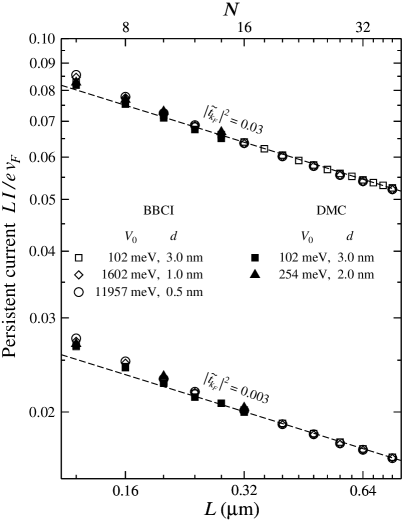
Figure 3: Persistent current $LI/ev_{F}$ versus the ring length $L$ for the ring with a single scatterer in the regime $LI\propto L^{-\alpha}$. Magnetic flux is $\phi=0.25\phi_{0}$, the electron density is $N/L=5\times 10^{7}$ m^-1. We compare the results for a scatterer with two various transmissions $|\tilde{t}_{k_{F}}|^{2}$. We also make comparison for various e-e interactions chosen so that the RG formula (56) predicts for each considered interaction the same $\alpha_{RG}$. Specifically, each set $(V_{0},d)$ listed in the figure is chosen so that the RG formula predicts $\alpha_{RG}(V_{0},d)=0.2565$. The dashed lines show the formula $LI\propto L^{-\alpha}$, where $\alpha={(1+2\alpha_{RG})}^{1/2}-1$ and the proportionality factor is specified in the text. The CI and DMC data are shown by symbols.

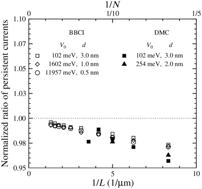
Figure 4: Data from figure 3 plotted as the ratio (59), where $I(\tilde{t}_{k_{F},1})$ and $I(\tilde{t}_{k_{F},2})$ are the persistent currents for $|\tilde{t}_{k_{F},1}|^{2}=0.03$ and $|\tilde{t}_{k_{F},2}|^{2}=0.003$, respectively.

In figure 3 we compare the persistent currents for two very different transmissions $|\tilde{t}_{k_{F}}|^{2}$ in order to demonstrate that the power $\alpha$ is universal - independent on the choice of $\tilde{t}_{k_{F}}$. Indeed, the CI and DMC data in figure 3 exhibit the same $\alpha$ for both transmissions.

One has to note that the formulae (4) and (6) are robust against the choice of the e-e interaction in the sense, that they give the same $\alpha$ for all e-e interactions with the same value of $[V(0)-V(2k_{F})]/v_{F}$. Obviously, this can be the case for many various choices of $V(x-x^{\prime})$.

To see whether such robustness exists in our many-body model, in figure 3 we also make comparison for various e-e interactions chosen so that the formula (56) gives for various sets $(V_{0},d)$ the value $\alpha_{RG}(V_{0},d)=0.2565$. Our CI and DMC data indeed show for all considered $(V_{0},d)$ the decay $LI\propto L^{-\alpha}$, where $\alpha={(1+2\alpha_{RG})}^{1/2}-1$ and $\alpha_{RG}=0.2565$. In summary, our methods seem to give the same $\alpha$ for various sets $(V_{0},d)$ fulfilling the equation $\alpha_{RG}(V_{0},d)=$const. Thus, our methods seem to confirm the above discussed robustness of the formulae (4) and (6) against the choice of the e-e interaction.

However, we will show later on that this robustness in fact holds only for the e-e interactions which are very short-ranged [all sets $(V_{0},d)$ in figure 3 actually belong to this special limit]. We know that we are in this limit as long as our methods confirm the formulae (4) and (6). This is still the case in the following discussion.

We specify the proportionality factor in the formula $LI\propto L^{-\alpha}$. Following the Introduction, we replace in the single-particle formula (1) the bare amplitude $\tilde{t}_{k_{F}}$ by the renormalized amplitude $t_{k_{F}}\propto(\tilde{t}_{k_{F}}/|\tilde{r}_{k_{F}}|)L^{-\alpha}$. We get

$$I=C\ \frac{ev_{F}}{2L}\ \frac{|\tilde{t}_{k_{F}}|}{|\tilde{r}_{k_{F}}|}\ L^{-\alpha}\sin(2\pi\phi/\phi_{0}),\quad\alpha>0,$$ (57)

where $C$ is the proportionality factor. Since $\alpha$ is universal (independent on $\tilde{t}_{k_{F}}$), the formula (57) implies that

$$\frac{I(\tilde{t}_{k_{F},1})}{I(\tilde{t}_{k_{F},2})}=\frac{|\tilde{t}_{k_{F},1}|/|\tilde{r}_{k_{F},1}|}{|\tilde{t}_{k_{F},2}|/|\tilde{r}_{k_{F},2}|}$$ (58)

as long as $C$ does not depend on $\tilde{t}_{k_{F}}$. To see that the CI and DMC data in figure 3 fulfill the equality (58), we show these data again in figure 4 in terms of the ratio

$$\frac{|\tilde{t}_{k_{F},2}|/|\tilde{r}_{k_{F},2}|}{|\tilde{t}_{k_{F},1}|/|\tilde{r}_{k_{F},1}|}\frac{I(\tilde{t}_{k_{F},1})}{I(\tilde{t}_{k_{F},2})},$$ (59)

which should equal unity for $L\rightarrow\infty$. One sees that it indeed approaches unity for the CI as well as DMC results. More precisely, the CI data show a few percent deviation from unity which tends to disappear with increasing $L$. A small deviation from unity show also the DMC data where convergence towards unity is not clear due to the stochastic noise of the Monte Carlo method.

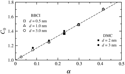
Figure 5: Dependence $C_{0}(\alpha)$ obtained by fitting the formula (60) to our CI and DMC data for $LI/ev_{F}$. Symbols show the fitted values of $C_{0}$. The dashed line is the function $C_{0}(\alpha)=1+1.66\alpha$ which fits the presented data points.

Thus, if we ignore a small finite-size effect in figure 4, our data in figure 3 are in accord with equation (58). Therefore, we can fit our data in the $L^{-\alpha}$ regime by the asymptotic formula (57). For the purpose of fitting it is useful to define $C\ \equiv{n_{e}}^{-\alpha}C_{0}$. Setting this definition into the formula (57) we obtain

$$\frac{LI}{ev_{F}}=\frac{1}{2}C_{0}(\alpha)\ \frac{|\tilde{t}_{k_{F}}|}{|\tilde{r}_{k_{F}}|}\ N^{-\alpha}\sin(2\pi\phi/\phi_{0}),$$ (60)

where $C_{0}$ depends solely on the parameter $\alpha$ (see below). Instead of (57) we use (60) and we fit $C_{0}$ instead of $C$.

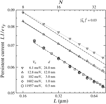
Figure 6: The circles, squares and diamonds are the BBCI data from the figure 3, the triangles and inverted triangles are the BBCI data for another two sets $(V_{0},d)$. For all considered $(V_{0},d)$, the formula (56) gives $\alpha_{RG}(V_{0},d)=0.2565$ and the formula (6) predicts $\alpha={(1+2\alpha_{RG})}^{1/2}-1=0.23$. However, the dependence $LI\propto L^{-0.23}$ (the dashed curves with different offset) can be seen to fit only the BBCI data for $d\leq 3$nm. The BBCI data for $d=12$nm are excellently fitted by the curve $LI\propto L^{-0.222}$ [the full line] and the BBCI data for $d=24$nm are fitted by $LI\propto L^{-0.207}$ [the dotted line]. This shows that the formulae (4) and (6) hold only for the e-e interactions which are very short-ranged (see the text).

The dashed lines in figures 2 and 3 show the dependence (60) fitted to the BBCI data in these figures. Specifically, $C_{0}$ is fitted and the function $N^{-\alpha}$ in (60) is evaluated by using $\alpha={(1+2\alpha_{RG})}^{1/2}-1$, where $\alpha_{RG}(V_{0},d)$ is given by the formula (56). The resulting values of $C_{0}$ are shown by open symbols in the figure 5. The full symbols in the figure 5 show the values of $C_{0}$ obtained when we fit by means of (60) the DMC data in figures 2 and 3. Also shown are the results obtained in the same way for another values of $\alpha$. Note that for all $(V_{0},d)$ giving the same $\alpha(V_{0},d)$ the obtained values of $C_{0}$ are essentially the same. This means that $C_{0}$ depends solely on the parameter $\alpha$. We also note that $C_{0}$ does not depend on $\tilde{t}_{k_{F}}$, as has been documented in the figure 4.

The linear fit in the figure 5,

$$C_{0}(\alpha)=1+1.66\alpha,$$ (61)

should be viewed as a first estimate of the analytical dependence. To extract a very precise formula for $C_{0}(\alpha)$, it would be desirable to simulate larger systems in order to better suppress the finite size effect in figure 4.

We conclude that the right-hand side of (60) depends on a single parameter $\alpha$ via the function $C_{0}(\alpha)N^{-\alpha}$, which is single-valued for various $(V_{0},d)$ giving the same $\alpha(V_{0},d)$. Our results confirm the decay $N^{-\alpha}$, where $\alpha$ is given by the formulae (6) and (4).

However, the formulae (6) and (4) in fact hold only for very small $d$. In the figure 6 we compare the BBCI data from the figure 3 with the BBCI data obtained for another two sets $(V_{0},d)$ with $d$ as large as $12$nm and $24$nm. All considered $(V_{0},d)$ are chosen so that the formulae (56) and (6) give for each $(V_{0},d)$ the same value of $\alpha$, in particular $\alpha=0.23$. However, it can be seen, that the dependence $LI\propto L^{-0.23}$ fits only the BBCI data for $d\leq 3$nm. The BBCI data for $d=12$nm and $d=24$nm are excellently fitted by the curves $LI\propto L^{-0.222}$ and $LI\propto L^{-0.207}$, respectively, i.e., with increasing $d$ our numerically obtained $\alpha$ decreases albeit the value of $\alpha_{RG}(V_{0},d)$ is fixed. This is a strong indication that the formulae (6) and (4) hold only for small $d$. We support this numerical finding by the following analytical proof.

$V_{0}$ (meV)	$d$ (nm)	$\alpha_{RG}$	$\alpha$	symbol in Fig. 7
11	3	0.0277	0.0273	$\circ$
34	3	0.0855	0.0821	$\circ$
68	3	0.171	0.158	$\circ$
1068	1	0.171	0.158	$\Box$
102	3	0.2565	0.230	$\circ$
1602	1	0.2565	0.230	$\Box$
11957	0.5	0.2565	0.230	$\triangle$
15942	1	0.342	0.298	$\Box$
15942	0.5	0.342	0.298	$\triangle$
3142	1	0.5	0.414	$\Box$
23445	0.5	0.5	0.414	$\triangle$

Table 2: The input parameters $V_{0}$ and $d$ used in the BBCI calculations of figure 7 and the values of $\alpha_{RG}$ and $\alpha$ resulting from the formulae (56) and (6). The last column of the table ascribes a symbol to each set $(V_{0},d,\alpha_{RG})$. These symbols are used in figure 7 to show the BBCI data.

In the appendix D we prove analytically that the matrix elements of the e-e interaction are independent on $d$ for $d\rightarrow 0$ at a fixed value of $\alpha_{RG}(V_{0},d)$. In other words, for $d\rightarrow 0$ the matrix elements depend on a single parameter $\alpha_{RG}$, otherwise they depend on two parameters $V_{0}$ and $d$. According to the appendix, the limit $d\rightarrow 0$ means $4k_{F}^{2}d^{2}\ll 1$. In our calculations $1/2k_{F}\simeq 3$nm and the currents in the figure 6 are close to each other for all $d\leq 3$nm. If we increase $\alpha_{RG}$ (for instance as in the table 2 and figure 7), we need to take $d<1/2k_{F}$ to see the $d$-independent current convincingly.

Note also another result in figure 6. As $d$ exceeds $1/2k_{F}$ the persistent current still decays like $LI\propto L^{-\alpha}$, but $\alpha$ depends on two parameters $V_{0}$ and $d$ rather than on a single one, $\alpha_{RG}$. This regime is not captured by the formulae (6) and (4). We have obtained similar results (not shown) also for other values of $\alpha_{RG}$.

Consider now a broader range of the e-e interaction parameters $V_{0}$ and $d$, listed in the table 2. The resulting persistent currents for these parameters are shown in the figure 7. All shown BBCI data asymptotically converge to the Luttinger-liquid behavior described by the formula (60), with the power $\alpha$ in accord with the formulae (6) and (4). We wish to stress the following aspects.

We can write (60) as $\frac{2LI}{ev_{F}C_{0}}=\frac{|\tilde{t}_{k_{F}}|}{|\tilde{r}_{k_{F}}|}x$, where $x\equiv N^{-\alpha}$ and $C_{0}(\alpha)$ is given by (61). Similarly, the BBCI data in the asymptotic regime can be normalized as $2LI/ev_{F}C_{0}$ and plotted as a function of the variable $x\equiv N^{-\alpha}$. This is done in inset to the figure 7. Indeed, all BBCI data in inset collapse to a single curve $f(x)=\frac{|\tilde{t}_{k_{F}}|}{|\tilde{r}_{k_{F}}|}x$. That a single linear curve involves the BBCI data for many various $N$, $V_{0}$ and $d$, is a clear sign of the Luttinger liquid with e-e interaction depending on one parameter $\alpha_{RG}$. It also documents that our calculations are reliable for a broad range of variables $N$, $V_{0}$ and $d$, the function $C_{0}(\alpha)$ is certainly determined with reasonable accuracy.

An interesting finding in figure 7 is that for large $\alpha_{RG}$ the BBCI data show the $LI\propto L^{-\alpha}$ decay already for ten electrons. In other words, the Luttinger-liquid behavior arises in the system with only ten particles. For comparison, in the lattice models Meden ; Enss-2005 ; Meden-2005 ; Andregassen the asymptotic power law is observed for a much larger number of electrons.

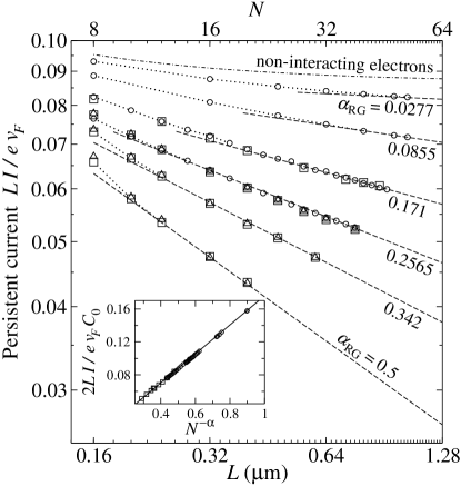
Figure 7: Persistent current versus the ring length for the same ring as in the figure 2, but for a broader range of the interaction parameters $V_{0}$ and $d$ (table 2). The circles, squares and triangles show the results of the BBCI method for various sets $(V_{0},d,\alpha_{RG})$ listed in the table 2. The dotted lines are a guide for eye. The dashed lines show the asymptotic law $LI\ \propto L^{-\alpha}$ plotted in the form (60), where $\alpha={(1+2\alpha_{RG})}^{1/2}-1$ and $\alpha_{RG}$ is obtained from (56). The BBCI data in the asymptotic regime are selected, normalized as $2LI/ev_{F}C_{0}$ [with $C_{0}(\alpha)$ given by the formula (61)], and plotted in inset as a function of the variable $x\equiv N^{-\alpha}$. The full line is the dependence $f(x)=\frac{|\tilde{t}_{k_{F}}|}{|\tilde{r}_{k_{F}}|}x$, predicted by the formula (60).

If we compare the formulae (60) and (1), we see that the interaction modifies the amplitude $\tilde{t}_{k_{F}}$ as

$$t_{k_{F}}\simeq(\tilde{t}_{k_{F}}/|\tilde{r}_{k_{F}}|)N^{-\alpha}=(\tilde{t}_{k_{F}}/|\tilde{r}_{k_{F}}|){(n_{e}^{-1}/L)}^{\alpha}.$$ (62)

This result scales with the length $n_{e}^{-1}$ while the RG result (3) scales with $d$. What is the origin of this difference? The RG result (3) should hold for any $d$ obeying the inequality (5), but the inequality (5) can in principle be fulfilled also for $d\lesssim 1/2k_{F}$, i.e., just for those $d$ for which we have obtained the formula (62). We think that the difference between the two results is due to the different physical models. The formula (62) holds in our continuous model, with the single-particle energy dispersion being truly parabolic. The RG formula (3) holds in the model Matveev , with the energy dispersion linearized in the interval $<\varepsilon_{F}-\hbar v_{F}/d,\varepsilon_{F}+\hbar v_{F}/d>$ around the Fermi energy. For small $d$ the band width $\hbar v_{F}/d$ becomes comparable with $\varepsilon_{F}$ and the model Matveev has a truly linear dispersion, like the Luttinger-liquid model Kane which also shows scaling by factor $(d/L)^{\alpha}$. For $d\gg 1/2k_{F}$ the linearization is unessential because of $\hbar v_{F}/d\ll\varepsilon_{F}$, hence both models should give the same results. The limit $d\gg 1/2k_{F}$ is however not feasible by our numerical methods for computational reasons.

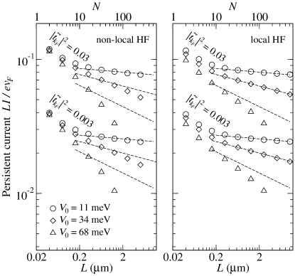
Figure 8: Persistent current $LI/ev_{F}$ versus ring length $L$ for the ring with single scatterer, calculated in the Hartree-Fock approximation for parameters $\phi=0.25\phi_{0}$, $N/L=5\times 10^{7}$ m^-1, $d=3$nm, and various $V_{0}$ and $|\tilde{t}_{k_{F}}|^{2}$ as listed in the figure. The left panel shows the nonlocal Hartree-Fock results, the right panel shows the Hartree-Fock results in the local Fock approximation (see the text). The Hartree-Fock results are shown by symbols, the dashed lines show the Luttinger liquid asymptotics $LI\ \propto L^{-\alpha}$, where $\alpha={(1+2\alpha_{RG})}^{1/2}-1$ and $\alpha_{RG}$ is given by the RG formula (56): $\alpha_{RG}=0.0277,0.0855$, and $0.1710$ for $V_{0}=11,34$, and $68$ meV, respectively.

III.2 Universal scaling in the Hartree-Fock model

Now we discuss the persistent currents obtained in the self-consistent Hartree-Fock approximation (Sect.IIC) which ignores correlations except for the Fock exchange.

In figure 8 we show the $I(L)$ dependence, calculated in the self-consistent Hartree-Fock approximation for the ring parameters already encountered in our correlated many-body calculations. The left panel shows the Hartree-Fock data obtained for the Fock term (33) treated as is, the right panel shows the Hartree-Fock data for the Fock term (33) approximated as Cohen-98 ; Cohen-97

$$U_{F}(x)\simeq-\sum\limits_{n^{\prime}}\int dx^{\prime}V(x-x^{\prime}){\rm Re}\left[\psi_{n^{\prime}}^{*}(x^{\prime})\psi_{n^{\prime}}(x)\right].$$ (63)

Unlike the nonlocal interaction (33) the approximation (63) is local - it does not depend on $n$. One readily obtains (63) from (33) by applying the ’almost closure relation’ $\sum_{n^{\prime}}\psi_{n^{\prime}}^{*}(x^{\prime})\psi_{n^{\prime}}(x)\simeq\delta(x-x^{\prime})$. Once this approximation is adopted, the final expression for the current has to be approximated correspondingly commentI .

Let us compare our Hartree-Fock calculations with the Luttinger liquid asymptotics $LI\ \propto L^{-\alpha}$. As can be seen in the figure 8, both Hartree-Fock approaches show the $I(L)$ dependence decaying for large $L$ faster than $L^{-1-\alpha}$. We will see below that for $L\rightarrow\infty$ the decay is in fact exponential. Only for the weak e-e interaction the Hartree-Fock data show the decay $L^{-1-\alpha}$, reported also in our previous Hartree-Fock studies Nemeth-2005 ; Gendiar . However, also in this case we expect exponential decay at very large $L$.

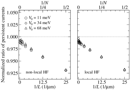
Figure 9: The Hartree-Fock data from the figure 8 plotted as the ratio (59), where $I(\tilde{t}_{k_{F},1})$ and $I(\tilde{t}_{k_{F},2})$ are the persistent currents for the transmission probabilities $|\tilde{t}_{k_{F},1}|^{2}=0.03$ and $|\tilde{t}_{k_{F},2}|^{2}=0.003$, respectively.

Now we show that also in the Hartree-Fock approximation the slope of $\log(I(L))$ becomes for $L\rightarrow\infty$ universal - dependent only on the e-e interaction. Following equations (57)-(59), such universality means that the ratio $\frac{|\tilde{t}_{k_{F},2}|/|\tilde{r}_{k_{F},2}|}{|\tilde{t}_{k_{F},1}|/|\tilde{r}_{k_{F},1}|}\frac{I(\tilde{t}_{k_{F},1})}{I(\tilde{t}_{k_{F},2})}$ approaches unity for $L\rightarrow\infty$. If we redraw in terms of this ratio the Hartree-Fock data from figure 8, we see (in the figure 9), that the ratio converges with increasing $L$ to unity. The stronger the interaction the better the convergence in the figure 9, for further improvement a further increase of $L$ is needed. Universality of the Hartree-Fock results in figure 9 is quite similar to the universality of the correlated results in figure 4.

Moreover, we would like to show that the Hartree-Fock model resembles the correlated model also in the following respect. In the limit $d\rightarrow 0$ the $I(L)$ curve is determined by a single e-e interaction parameter $\alpha_{RG}$ [i.e., $I(L)$ is the same for various $(V_{0},d)$ giving the same value of $\alpha_{RG}(V_{0},d)$]. This is demonstrated in the figure 10.

Figure 10 shows the Hartree-Fock results for the weak and strong e-e interactions. Also shown are the corresponding correlated results from the figure 2, in particular the BBCI data (full lines) and the Luttinger-liquid curves (dashed lines). Note the following details.

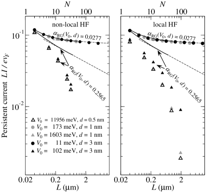
Figure 10: Length-dependence of the persistent current in the ring with single scatterer, obtained in the Hartree-Fock approximation. The Hartree-Fock results are shown by symbols. The ring parameters are: $\phi=0.25\phi_{0}$, $N/L=5\times 10^{7}$ m^-1, and $|\tilde{t}_{k_{F}}|^{2}=0.03$. The weak and strong e-e interactions are simulated for various $(V_{0},d)$ obeying the equations $\alpha_{RG}(V_{0},d)=0.0277$ and $\alpha_{RG}(V_{0},d)=0.2565$, respectively, where $\alpha_{RG}(V_{0},d)$ is given by the RG formula (56). Also shown are the corresponding BBCI data (full lines) and asymptotic $LI\ \propto L^{-\alpha}$ curves (dashed lines), taken from the figure 2.

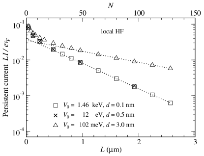
Figure 11: Length-dependence of the persistent current in the ring with single scatterer, obtained in the local Hartree-Fock approximation. The Hartree-Fock data are shown by symbols. The ring parameters are: $\phi=0.25\phi_{0}$, $N/L=5\times 10^{7}$ m^-1, and $|\tilde{t}_{k_{F}}|^{2}=0.03$. The parameters of the e-e interaction, $V_{0}$ and $d$, are listed in the figure. The considered sets $(V_{0},d)$ obey the equation $\alpha_{RG}(V_{0},d)=0.2565$, where $\alpha_{RG}(V_{0},d)$ is given by the RG formula (56). For large $L$ the current decays with $L$ linearly, but note that the scale is semi-logarithmic. The dotted lines fit linearly the Hartree-Fock data at large $L$.

For weak e-e interaction ($\alpha_{RG}=0.0277$) the Hartree-Fock data are robust against various $(V_{0},d)$ obeying the equation $\alpha_{RG}(V_{0},d)=0.0277$. This is illustrated by the agreement of the Hartree-Fock data for ($V_{0}=173$meV, $d=1$nm) and ($V_{0}=11$meV, $d=3$nm). Note also that these Hartree-Fock data almost reproduce the correlated results at sizes $L$ considered in the figure. To obtain conclusions valid for any $L$ and any interaction strength, we have to look at the stronger e-e interaction.

For strong e-e interaction ($\alpha=0.2565$) the Hartree-Fock data fail to agree with the correlated results. However, the Hartree-Fock data still tend to be robust against various $(V_{0},d$) obeying the equation $\alpha_{RG}(V_{0},d)=0.2565$ in the limit $d\rightarrow 0$. This universal dependence on a single e-e interaction parameter $\alpha_{RG}$ is clearly visible both in the nonlocal and local Hartree-Fock calculation.

Finally, we would like to show that the decay of $I(L)$ in the Hartree-Fock approximation is exponential for large $L$. This exponential decay is demonstrated in the figure 11, where the $I(L)$ dependence is presented in the semi-logarithmic scale. We need to consider large $L$ and strong e-e interaction, which strongly prolongs the time of the Hartree-Fock computation. Fortunately, the calculation is feasible in the local approximation (63).

The $I(L)$ curves in figure 11 do not decay equally fast, albeit the value of $\alpha_{RG}(V_{0},d)$ is the same for all considered $(V_{0},d)$. It can however be seen that if we keep the same value of $\alpha_{RG}(V_{0},d)$ in the limit $d\rightarrow 0$, then the slope of $I(L)$ is determined solely by the value of $\alpha_{RG}$. This is again a clear manifestation of the universal dependence on a single e-e interaction parameter. The limit $d\rightarrow 0$ is well represented by the data for $d=0.1$nm.

In summary, our self-consistent Hartree-Fock results show, that the slope of $\log(I(L))$ in the limit of large $L$ is still universal - dependent solely on the e-e interaction not on the strength of the scatterer. Moreover, for $d\rightarrow 0$ this dependence on the e-e interaction is determined by a single e-e interaction parameter, specifically by $\alpha_{RG}$ given by the RG formula (56). These features are very similar to the universal behavior observed in our correlated calculations. A major difference is that in the Hartree-Fock approximation the asymptotic decay of $I(L)$ is exponential with $L$, as we have shown numerically.

III.3 Reliability and limitations of the CI and DMC

Both DMC and CI methods in their most rigorous formulations show exponential scaling of the computer time in the number of particles. In CI this is due the necessity of infinite size of the basis and high level of excitations which are required to make the method size consistent Szabo ; Jensen . In practice, for not too large systems, useful and accurate results can be obtained providing a sufficiently large set of virtual orbitals can be treated. The question is whether the low-order (doubles, triples, quadruples) excitations are enough to capture the key many-body effects. For the DMC method, the exponential scaling originates in the fermion sign problem which is in practice avoided by the fixed-node or fixed-phase approximations. The usefulness of the method crucially relies on accuracy of the trial functions and ability to efficiently describe the impact of the many-body effects on accuracy of the nodes or phase Foulkes-01 . The DMC practice shows that very large systems can be treated nevertheless the fixed-node/phase bias is present and it depends on phenomena of interest whether it can affect the results.

In subsection IIIA, the largest many-body systems ($48$ electrons) were simulated by the CI method while only at most $32$ electrons were simulated by the DMC. This is caused by the fact that the phase of the Hartree-Fock wave function becomes less accurate with increasing strength of the interaction and also with increasing size of the system. This is not too difficult to understand since in larger and strongly interacting systems the collective excitations become more complicated and the single determinant wave function becomes very poor representation of the actual ground state. The many-body effects description built into the trial function thus directly determines the accuracy of the obtained results.

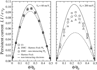
Figure 12: Persistent current versus magnetic flux for the GaAs ring with $N=4$ and $L=N/n_{e}=80$ nm. The transmission of the scatterer is $|\tilde{t}_{k_{F}}|^{2}=0.03$. The e-e interaction range is set to $d=3$ nm and the e-e interaction magnitude is $V_{0}=68$ meV in the left panel and $V_{0}=200$ meV in the right panel. The triangles show the results of the fixed-phase DMC calculation with the trial wave function $\Psi_{T}(\textbf{X})$ equal to the Slater determinant (29) of the self-consistently determined Hartree-Fock ground state. The squares show the results of the fixed-phase DMC calculation with the trial wave function $\Psi_{T}(\textbf{X})$ equal to the Slater determinant of the non-interacting ground state. The CI results are shown by circles connected by the dotted line. For completeness, the results for the non-interacting ground state are shown in a full line and the results of the self-consistent Hartree-Fock calculation are shown in a dashed line.

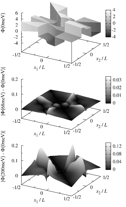
Figure 13: Comparison of various phases from the DMC calculations of figure 12 at $\phi=0.25\phi_{0}$. The top panel shows the phase $\Phi(x_{1},x_{2},x_{3},x_{4})$ of the non-interacting trial wave function $\Psi_{T}(x_{1},x_{2},x_{3},x_{4})$ evaluated at $x_{3}=-L/6$ and $x_{4}=L/6$. It is labelled as $\Phi(0\text{meV})$ since it holds for $V_{0}=0$meV. The middle panel shows the phase difference $|\Phi(68\text{meV})-\Phi(0\text{meV})|$, where $\Phi(68\text{meV})$ is the phase $\Phi(x_{1},x_{2},x_{3}=-L/6,x_{4}=L/6)$ of the trial wave function $\Psi_{T}(x_{1},x_{2},x_{3},x_{4})$ obtained for $V_{0}=68$meV by the Hartree-Fock method. The bottom panel shows the phase difference $|\Phi(200\text{meV})-\Phi(0\text{meV})|$. We note that the abrupt change of the phase for $x_{i}=x_{j}$ arises because the Slater determinant changes abruptly its sign for $x_{i}\leftrightarrow x_{j}$.

In figure 12 we show the persistent current versus magnetic flux for the ring with four electrons. The range of the e-e interaction is $d=3$nm, the e-e interaction magnitude is $V_{0}=68$meV in the left panel and $V_{0}=200$meV in the right panel. The triangles represent the DMC calculation with the trial wave function $\Psi_{T}(\textbf{X})$ equal to the Slater determinant (29) of the Hartree-Fock ground state. The squares show the DMC calculation with the trial wave function equal to the Slater determinant of the non-interacting ground state. The results of both DMC calculations are very close when $V_{0}=68$meV, but they are very different when $V_{0}=200$meV. This suggests that the DMC results for $V_{0}=200$meV are strongly affected by the phase of the trial wave function. Indeed, for $V_{0}=68$meV both DMC calculations essentially agree with the corresponding CI calculation (circles), but for $V_{0}=200$meV the differences with the CI data are very clear.

It is interesting to see the origin of the fixed-phase biases. For illustration, in figure 13 we compare the phases involved in the DMC calculations of figure 12. The phase difference $|\Phi(68\text{meV})-\Phi(0\text{meV})|$ is small and this is why the corresponding DMC currents in the left panel of figure 12 almost coincide. The phase difference $|\Phi(200\text{meV})-\Phi(0\text{meV})|$ is large and the corresponding DMC currents in the right panel of figure 12 clearly differ.

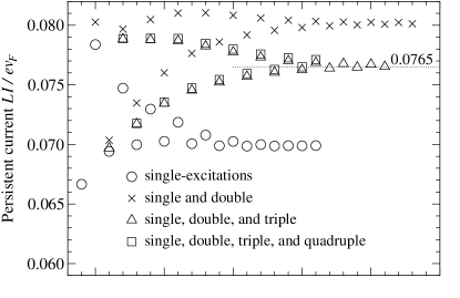
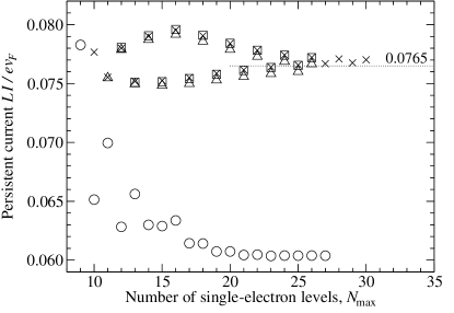
Figure 14: Convergence of the persistent current in the FCI calculation in dependence on the number of the considered single-electron levels for the single-excitations, single- and double-excitations, etc. The top panel shows the currents obtained from the formula $I=\left<\Psi_{0}\right|\hat{I}\left|\Psi_{0}\right>$, the bottom panel shows the currents obtained in the same FCI calculation from the formula $I=-\partial E_{0}/\partial\phi$. The results are shown by symbols. They were obtained for the ring with parameters $N=8$ and $L=N/n_{e}=0.16$ $\mu$m, penetrated by magnetic flux $\phi=0.25\phi_{0}$. The transmission of the scatterer is $|\tilde{t}_{k_{F}}|^{2}=0.03$. The e-e interaction is given by $V_{0}=102$ meV and $d=3$ nm.

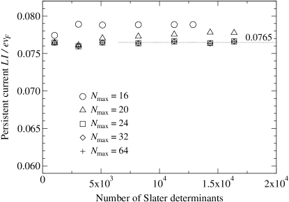
Figure 15: Convergence of the persistent current in the BBCI calculation for various $N_{max}$ in dependence on the number of the Slater determinants involved in the expansion (52). We recall that the determinants are selected by using the bucket-brigade algorithm of Appendix C and $N_{max}$ is the number of the considered single-electron levels. In this BBCI calculation the current is evaluated by using the formula $I=\left<\Psi_{0}\right|\hat{I}\left|\Psi_{0}\right>$ and the parameters of the ring are the same as in the FCI calculation of the preceding figure. The value $0.0765$ is the average from the (well saturated) data for $N_{max}\geq 24$.

We conclude that the main limitation of our DMC results is the Hartree-Fock approximation of the correct phase, which deteriorates with increase of the e-e interaction and system size. In particular, we see in the figure 12 that the DMC with the Hartree-Fock trial wave function underestimates the persistent current. For instance, in figure 2 the DMC data for the $\alpha_{RG}=0.2565$ exhibit a weak underestimation which is of the same origin.

Reliability of the CI results depends on how the results converge with increasing the number of the Slater determinants in the expansion (52).

The figure 14 shows a typical convergence process in the FCI calculation. We recall that we add into the expansion (52) first the Slater determinant of the ground state, then all determinants with a single excited electron (the single-excitations), all determinants with two excited electrons (the double-excitations), etc. The figure 14 demonstrates how the persistent current saturates with increasing the size of the single-electron basis (the number of the considered single-electron levels) for the single-excitations only, for the single- and double-excitations, etc. Moreover, the top and bottom panel compare convergence of the persistent currents calculated by means of the formulae $I=\left<\Psi_{0}\right|\hat{I}\left|\Psi_{0}\right>$ and $I=-\partial E_{0}/\partial\phi$, respectively. It can be seen that both approaches converge to the same final result when the single-, double-, triple-, and quadruple-excitations are considered. However, precision of the results in the bottom panel is good already for the single- and double-excitations while in the top panel also the triple-excitations are needed to achieve a comparable precision.

The FCI calculations with the formula $I=-\partial E_{0}/\partial\phi$ therefore consume much less computer time and memory. The FCI data presented in this text were obtained by means of the formula $I=-\partial E_{0}/\partial\phi$ and by considering the single- and double-excitations. In a few cases, sufficiency of the achieved convergence was confirmed by adding the triple-excitations or even the quadruple-excitations, with a similar success as in the figure 14.

The figure 15 shows typical convergence of the BBCI calculation in dependence on the number of the Slater determinants involved in the expansion (52). The persistent currents in the BBCI converge to the value $0.0765$, in accord with the value reached by the FCI data in figure 14. The BBCI data in this text were obtained by using the formula $I=\left<\Psi_{0}\right|\hat{I}\left|\Psi_{0}\right>$. The BBCI relying on the formula $I=-\partial E_{0}/\partial\phi$ gives the same results (not shown), but the computational time is about twice longer.

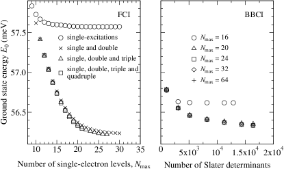
Figure 16: The left panel shows how the ground-state energy $E_{0}$ converges in the FCI calculation of figure 14. The right panel shows how $E_{0}$ converges in the BBCI calculation of figure 15.

In figure 16 we demonstrate convergence of the ground-state energy $E_{0}$ in the FCI (left panel) and BBCI calculation (right panel). In both cases $E_{0}$ converges to a certain minimum. Here $E_{0}$ is better minimized in the FCI calculation than in the BBCI, but we note that the BBCI result would eventually converge (for a significantly larger number of determinants) to the same minimum. In both cases, however, we need to add more determinants to achieve a perfectly saturated $E_{0}$. In contrast to this, if we look at the convergence of the corresponding persistent currents (figures 14 and 15, respectively), we see that it is satisfactory finished both in the FCI and BBCI. Thus, as long as we are interested in the persistent current, it is economical to look at the convergence of the current rather than at the convergence of $E_{0}$.

In figure 17 we show the ground-state energy and persistent current as functions of magnetic flux for the same parameters as in figures 14, 15, and 16. The CI and DMC results for the currents are in good agreement. However, the CI and DMC ground-state energies exhibit small differences which deserve a comment. In particular, in spite of the fixed-phase approximation the DMC ground-state energy shows the best minimum. The reasons for this are the following. First, the FCI results in the figure 17 were obtained by including the single, double, and triple-excitations (see the discussion of figures 14 and 16). The quadruple-excitations, etc., would shift the FCI ground-state energy to a slightly lower value. Second, the presented BBCI results were obtained for $N_{max}=64$ and for $1.6\times 10^{4}$ Slater determinants (see figures 15 and 16). Inclusion of more determinants would shift the BBCI ground-state energy to a lower value.

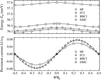
Figure 17: The ground-state energy $E_{0}$ and persistent current as functions of magnetic flux for the ring with parameters $N=8$ and $L=N/n_{e}=0.16$ $\mu$m. The transmission of the scatterer is $|\tilde{t}_{k_{F}}|^{2}=0.03$. The parameters of the e-e interaction are $V_{0}=102$ meV and $d=3$ nm, they give $\alpha_{RG}=0.2565$. The CI, DMC and Hartree-Fock (HF) results are shown by symbols. The full lines are a guide for eye, the dashed line shows the formula (60), with $\alpha={(1+2\alpha_{RG})}^{1/2}-1$ in the function $N^{-\alpha}$ and with the value of $C_{0}$ taken from figure 5.

It is tempting to think that the result showing the lowest ground-state energy is the best one. Such criterion indeed follows from the variational principle if we compare various methods applied to the same Hamiltonian. Here the CI methods are applied to the exact Hamiltonian but the DMC is applied to the effective Hamiltonian. If the ground-state energy of the effective Hamiltonian is lower than the ground-state energy of the exact Hamiltonian, this is not in conflict with the variational principle. It should also be stressed that the convergence of other properties such as expectation value of the current operator is not necessarily governed by the same behavior as the energy convergence. We believe that our CI results are closer to the true ones due to the good CI convergence demonstrated above. On the other hand the crude Hartree-Fock wave functions used in the fixed-phase approximation are probably not accurate enough to provide accurate currents for strongly interacting limit. This remains an interesting point for future studies since more accurate trial wave functions can be constructed by means of pairing orbitals and pfaffians, expansions in pfaffians and/or using backflow (dressed) many-body coordinates Bajdich08 .

IV Summary and concluding remarks

We have studied the persistent current of the interacting spinless electrons in a continuous 1D ring with a single strongly reflecting scatterer. We have included correlations by solving the Schrodinger equation for several tens of electrons interacting via the pair interaction $V(x-x^{\prime})=V_{0}\,\exp(-\left|x-x^{\prime}\right|/d)$. Our aim was to solve this continuous many-body problem without any physical approximation and to examine microscopically the power-law behavior of the Luttinger liquid. We have used advanced CI and DMC methods which, unlike the Luttinger-liquid model, do not rely on the Bozonization technique.

In the past, similar studies were performed by numerical RG methods in the lattice model Meden ; Enss-2005 ; Meden-2005 ; Andregassen . Our methods do not rely on the RG techniques and thus serve as independent confirmation of such approaches. Moreover, dealing with the continuous model, we can vary the range of the e-e interaction in order to test the robustness of the Luttinger-liquid power laws against various shapes of $V(x-x^{\prime})$. This point was not addressed in the lattice-model studies as the range of the interaction was usually fixed to the on-site interaction and/or to the nearest-neighbor-site interaction. Our major findings are:

(i) Our CI and DMC calculations confirm that the persistent current exhibits the asymptotic power-law behavior of the Luttinger liquid, $I\propto L^{-1-\alpha}$.

(ii) In our continuous model, the question whether the power $\alpha$ is determined by a single e-e interaction parameter $\alpha_{RG}$ is addressed by using various shapes of $V(x-x^{\prime})$ giving the same value of $\alpha_{RG}$. Our numerical values of $\alpha$ confirm the theoretical formula $\alpha={(1+2\alpha_{RG})}^{1/2}-1$ with $\alpha_{RG}$ given by the RG expression (4), but only if the range of $V(x-x^{\prime})$ is small ($d\lesssim 1/2k_{F}$).

(iii) The CI data for $\alpha_{RG}\gtrsim 0.3$ show onset of the asymptotics $I\propto L^{-1-\alpha}$ already for ten electrons. In other words, the Luttinger-liquid behavior emerges in the system with only ten particles. For comparison, a far much larger number of electrons is needed to observe the asymptotic power law in the lattice model Meden ; Enss-2005 ; Meden-2005 ; Andregassen . To understand origin of this difference, it would be desirable to study smooth transition from the lattice model to the continuous model.

(iv) We have treated the e-e interaction in the self-consistent Hartree-Fock approximation. We observe for large $L$ the exponentially decaying $I(L)$ instead of the power law. However, the slope of $\log(I(L))$ still depends solely on the parameter $\alpha_{RG}$ given by the RG formula (4), as long as the range of $V(x-x^{\prime})$ approaches zero.

(v) We have discussed the reliability and limits of our CI and DMC calculations. The CI methods appear to provide convergent results for the sizes and strengths of interactions we have studied. The reliability of the FCI and BBCI results is easy to analyze in this case and both methods converge to the same results although the BBCI can treat larger systems. The main limitation of our DMC calculations is the accuracy of Hartree-Fock trial function phase which has been employed in the fixed-phase calculations and appears to be a rather poor approximation for strong e-e interaction.

Figure 18: Electron-electron interaction versus distance in the GaAs 1D system. The dotted line shows the bare e-e interaction $V_{\text{bare}}(x-x^{\prime})=\frac{e^{2}}{4\pi\epsilon}\,\frac{1}{\left|x-x^{\prime}\right|+x_{0}}$ for $\epsilon=12.5\epsilon_{0}$ and $x_{0}=3$ nm, where the cutoff $x_{0}$ mimics the finite wire thickness. The thin full line shows the potential of a single electron screened by the free 1D electron gas, calculated in the Hartree picture comment2 . The full line is the best fit by formula $V(x-x^{\prime})=V_{0}\,e^{-\left|x-x^{\prime}\right|/d}$, where $d=3$nm essentially coincides with the value of $1/2k_{F}$. We expect that external gates would further increase the screening, i.e., it is indeed meaningful to focus on the range $d\lesssim 1/2k_{F}$ as we did in our work. The Friedel oscillations in the figure are artefact of static screening and would be further suppressed by the gates.

Although our work is not aimed to address experimental aspects, nevertheless, one of our findings might be a motivation for experimental work. It might be interesting to observe onset of the Luttinger-liquid behavior in the 1D system with a small number of strongly interacting electrons, e.g. with only ten electrons as predicts our work. In this respect we mention, that the screened e-e interaction (7) with the parameters $V_{0}$ and $d$ considered in our calculations is quite realistic. This is documented in figure 18, where the model interaction (7) is compared with the microscopic Hartree screening of the bare e-e interaction.

V Acknoledgement

The IEE group was supported by the grant APVV-51-003505, grant VEGA 2/6101/27, and ESF project VCITE. L. M. thanks for support from NSF and DOE.

Appendix A: Numerical algorithm for calculation of amplitudes $t_{k}$ and $r_{k}$

Consider again the segment $\langle-L/2,L/2\rangle$ embedded between two perfect semi-infinite leads. Outside the segment the electron wave function reads

$$\varphi_{k}(x)=e^{ikx}+r_{k}e^{-ikx},\ \varphi_{k}(x)=t_{k}e^{ikx}$$ (64)

for the electron impinging the segment from the left and

$$\varphi_{-k}(x)=t^{\prime}_{k}e^{-ikx},\ \varphi_{-k}(x)=e^{-ikx}+r^{\prime}_{k}e^{ikx}$$ (65)

for the electron impinging the segment from the right, where $k>0$, $r_{k}$ is the reflection amplitude, and $t_{k}$ is the transmission amplitude. Therefore, the boundary conditions for elastic tunneling through the segment $\langle-L/2,L/2\rangle$ have a standard form

$$\varphi_{k}(-\frac{L}{2})=e^{-ik\frac{L}{2}}+r_{k}e^{ik\frac{L}{2}},\ \varphi_{k}(\frac{L}{2})=t_{k}e^{ik\frac{L}{2}},$$ (66)

$$\varphi_{-k}(-\frac{L}{2})=t^{\prime}_{k}e^{ik\frac{L}{2}},\ \varphi_{-k}(\frac{L}{2})=e^{-ik\frac{L}{2}}+r^{\prime}_{k}e^{ik\frac{L}{2}}.$$ (67)

To calculate $t_{k}$ and $r_{k}$, we have to solve equation (11) as a tunneling problem with boundary conditions (66). We write equation (11) in the discrete form (21). Consider now the electron with $k>0$. It leaves the segment $\langle-L/2,L/2\rangle$ at $x=L/2$ as a free wave $\propto e^{ikL/2}$. We can thus initialize the scheme (21) at $x=L/2+\Delta$ and $x=L/2$ by using

$$\varphi_{k}^{\text{num}}\left(L/2+\Delta\right)=e^{ik(L/2+\Delta)},\quad\varphi_{k}^{\text{num}}\left(L/2\right)=e^{ikL/2}.$$

By means of (21) we generate the numerical solution $\varphi_{k}^{\text{num}}\left(x_{j}\right)$ starting at $x=L/2-\Delta$ and ending at $x=-L/2$. Since $\varphi_{k}\left(L/2\right)=t_{k}\varphi_{k}^{\text{num}}\left(L/2\right)$, the correctly scaled result is $\varphi_{k}\left(x\right)=t_{k}\varphi_{k}^{\text{num}}\left(x\right)$, where $t_{k}$ is yet unknown. We can readily express $t_{k}$ and $r_{k}$ from the boundary condition

$$t_{k}\,\varphi_{k}^{\text{num}}\left(x\right)=e^{ikx}+r_{k}\,e^{-ikx},\quad x=-\frac{L}{2},$$ (68)

and from the flux continuity equation

$$t_{k}\frac{d}{dx}\,\varphi_{k}^{\text{num}}\left(x\right)=\frac{d}{dx}\,\left[e^{ikx}+r_{k}\,e^{-ikx}\right],\quad x=-\frac{L}{2}.$$ (69)

A similar procedure can be used to obtain the solution $\varphi_{-k}\left(x\right)$ together with the amplitudes $t^{\prime}_{k}$ and $r^{\prime}_{k}$.

Appendix B: Iteration steps of the Hartree-Fock calculation

For numerical purposes it is useful comment1 to replace the potential $\gamma\delta(x)+U_{H}(x)+U_{F}(n,x)$ in the Hartree-Fock equation (35) by the potential

$$U_{new}(n,x)=f[\gamma\delta(x)+U_{H}(x)+U_{F}(n,x)]\\ +(1-f)U_{old}(n,x)\,.$$ (70)

In a given iteration step the equation (35) is solved with the potential $U_{new}(n,x)$, where $U_{old}$ is $U_{new}$ from the previous iteration step, and $f<1$ is a properly chosen weight. In the first iteration step we set $U_{new}\equiv\gamma\delta(x)$.

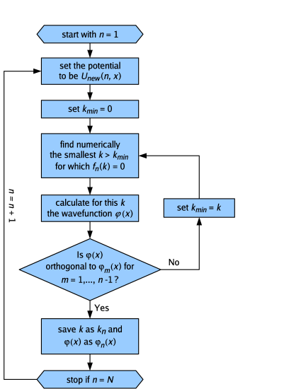
Figure 19: Flowchart of a single Hartree-Fock iteration step as described in the text.

The iteration step works as follows. We search for the Hartree-Fock energies $\varepsilon_{n}$ by solving the equation (19). Precisely, we solve the equation $f_{n}(k)=0$, where

$$f_{n}(k)={\rm Re}\{e^{-ikL}/t_{k}\}-\cos(2\pi\phi/\phi_{0})$$ (71)

and $t_{k}$ is the transmission evaluated for the potential $U_{new}(n,x)$. Clearly, the equation $f_{n}(k)=0$ is fulfilled for many different values of the variable $k$. Among these values we choose as physically correct only those $k=k_{n}$ which fulfill simultaneously two conditions. The first condition is the inequality $\varepsilon_{1}<\varepsilon_{2}<\dots<\varepsilon_{N}$, where $\varepsilon_{1},\varepsilon_{2},\dots\varepsilon_{N}$ are the energies of the $N$ lowest levels, each of them given as $\varepsilon_{n}=\hbar^{2}k_{n}^{2}/2m$. The second condition is that the wave functions $\varphi_{n}(x)$ of these $N$ lowest levels are mutually orthogonal. The flowchart of the iteration step is shown in the figure 19.

After finishing the iteration step we set the obtained $\varphi_{n}(x)$ into the potentials $U_{H}(x)$ and $U_{F}(n,x)$ and we obtain $U_{new}(n,x)$ for the following iteration step. We repeat the iteration steps until the energies $\varepsilon_{n}$ do not change anymore.

We note that we calculate the transmission $t_{k}$ for the given $U_{new}(n,x)$ by means of the algorithm from Appendix A. The wave function $\varphi_{n}(x)$ of the energy level $\varepsilon_{n}=\hbar^{2}k_{n}^{2}/2m$ is calculated by using the procedure described in the last paragraph of Section II.A.

Appendix C: Implementation of BBCI

Here we outline the BBCI algorithm Indlekofer . As mentioned in section II.E, we determine the single-particle basis $\psi_{j}(x)$ with the ladder of the single-particle-energy levels $\varepsilon_{j}$ and we consider only the first $N_{max}$ levels by introducing the upper energy cutoff as illustrated in the figure 1. Due to the cutoff, the expansion (52) contains the finite number of the Slater determinants $\chi_{n}$. This number, equal to $\left({N_{max}}\atop{N}\right)$ by simple combinatorics, is usually huge. The question is how to asses the importance of all $\left({N_{max}}\atop{N}\right)$ determinants and to omit those of them which are unimportant. In principle, the importance criterion adopted in section II.E requires to compute the energy $\left<\chi_{n}\right|\hat{H}\left|\chi_{n}\right>$ for all $\left({N_{max}}\atop{N}\right)$ determinants and to order the obtained numerical values $\left<\chi_{n}\right|\hat{H}\left|\chi_{n}\right>$ increasingly. Since $\left({N_{max}}\atop{N}\right)$ is huge, such direct approach still consumes enormous amount of the computer memory and it is also time-consuming to order increasingly a series of $\left({N_{max}}\atop{N}\right)$ numbers. The bucket-brigade algorithm Indlekofer eliminates these difficulties as follows.

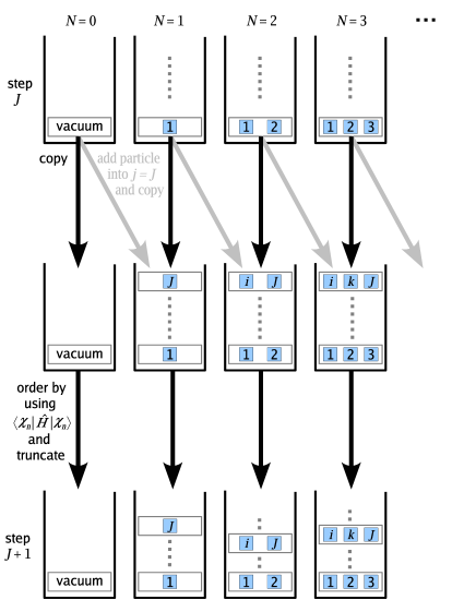
Figure 20: Visualization of the recursion step $J\rightarrow J+1$ discussed in the text: Copy the remaining (after truncation) Slater determinants from the $N$-particle bucket in step $J$ into the $N$-particle bucket in step $J+1$. Copy the remaining (after truncation) Slater determinants from the $(N-1)$ -particle bucket in step $J$ into the $N$-particle bucket in step $J+1$, but, when copying, enlarge each Slater determinant by creating a particle in the state $j=J$. Truncate with the help of the measure $\left<\chi_{n}\right|\hat{H}\left|\chi_{n}\right>$ the Slater determinants of each bucket in the step $J+1$. Go to the step $J+2$. Stop the procedure after $J$ reaches $N_{max}$. The squares represent the occupied single-particle states $j=1,2,\dots,J$. The number of the particles in the bucket is labelled by $N$.

We use the single-particle states $\psi_{j}(x)$ to generate the Slater determinants $\chi_{n}$ via a recursion algorithm (Fig. 20) which is based on the sequence of buckets $S_{J,N}$ with $J=0,\cdots,N_{max}$ and $N=0,\cdots,N_{max}$, where $N$ is the number of the particles in the bucket and $J$ labels the recursion step $J\rightarrow J+1$. Each bucket $S_{J,N}$ contains only the Slater determinants of $N$ particles which occupy the single-particle states $\psi_{j}(x)$ with $j=0,\cdots,J-1$. In each recursion step $J\rightarrow J+1$, we first expand the old buckets $S_{J,N}$ by adding the Slater determinants from the buckets $S_{J,N-1}$, but with an extra particle created in the single-particle state $j=J$. After this expansion, the buckets $S_{J+1,N}$ are truncated by selecting only the most important Slater determinants in accord with our importance criterion based on the chosen measure of importance, which is chosen as $\left<\chi_{n}\right|\hat{H}\left|\chi_{n}\right>$ in this paper. Owing to this algorithm our importance criterion is applied only to the determinants in the bucket rather than to all $\left({N_{max}}\atop{N}\right)$ determinants.

Appendix D: Matrix elements of electron-electron interaction

If we expand the function $f(x+y)$ into the Taylor series around $x$, we can write

$$\int\limits_{-L/2}^{L/2}{\rm d}yV(y)f(x+y)=\sum_{n=0}^{\infty}v_{n}f^{(n)}(x)\,,$$ (72)

where $f^{(n)}(x)=\frac{\partial^{n}}{\partial x^{n}}f(x)$ and

$$v_{n}=\frac{1}{n!}\int\limits_{-L/2}^{L/2}{\rm d}yV(y)y^{n}\,.$$ (73)

Setting the short range interaction $V(y)=V_{0}e^{-|y|/d}$ into (73) we get

$$v_{n}=\frac{V_{0}}{n!}\int\limits_{-L/2}^{L/2}{\rm d}ye^{-|y|/d}y^{n}=\frac{V_{0}}{n!}[1+(-1)^{n}]\int\limits_{0}^{L/2}{\rm d}ye^{-y/d}y^{n}$$ (74)

and after integration per partes we obtain

$$v_{n}=V_{0}d\,[1+(-1)^{n}]\!\left[d^{n}-e^{-L/2d}\sum_{m=0}^{n}\frac{d^{m}(L/2)^{n-m}}{(n-m)!}\right]\,.$$ (75)

Setting this $v_{n}$ back into (72), reordering the summations over $m$ and $n$, identifying the particular Taylor series of $f^{(n)}(x\pm L/2)$, and using the periodicity condition $f^{(n)}(x\pm L)=f^{(n)}(x)$, we obtain the relation

$$\int\limits_{-L/2}^{L/2}{\rm d}yV_{0}e^{-|y|/d}f(x+y)=\\ 2V_{0}d\sum_{n=0}^{\infty}d^{2n}\left[f^{(2n)}(x)-e^{-L/2d}f^{(2n)}(x-L/2)\right]\,.$$ (76)

In the limit $L\gg d$ this relation simplifies to

$$\int\limits_{-L/2}^{L/2}{\rm d}yV_{0}e^{-|y|/d}f(x+y)\approx 2V_{0}d\sum_{n=0}^{\infty}d^{2n}f^{(2n)}(x)\,.$$ (77)

Using the relation (77) and substitution $z=2\pi x/L$ we can rewrite the matrix elements

$$V_{ij}=\frac{1}{2}\sum\limits_{\alpha,\beta,\gamma,\delta}a_{ij\alpha\beta\gamma\delta}V_{\alpha\beta\gamma\delta}$$ (78)

with $a_{ij\alpha\beta\gamma\delta}$ being one of the values $\{-1,0,1\}$ and with

$$V_{\alpha\beta\gamma\delta}=\\ V_{0}\!\!\int\limits_{-L/2}^{L/2}\!\!\!{\rm d}x\;\psi_{\alpha}^{*}(x)\psi_{\gamma}(x)\!\!\int\limits_{-L/2}^{L/2}\!\!\!{\rm d}y\;e^{-|y|/d}\,\psi_{\beta}^{*}(x+y)\psi_{\delta}(x+y)$$ (79)

into the form

$$V_{ij}\approx V_{0}d\frac{L}{2\pi}\sum_{n=0}^{\infty}\left(\frac{2\pi d}{L}\right)^{2n}A_{ijn}\,,$$ (80)

where

$$A_{ijn}=\sum\limits_{\alpha,\beta,\gamma,\delta}a_{ij\alpha\beta\gamma\delta}\int\limits_{-\pi}^{\pi}\!\!\!{\rm d}z\;\psi_{\alpha}^{*}(z)\psi_{\gamma}(z)\frac{\partial^{2n}}{\partial z^{2n}}[\psi_{\beta}^{*}(z)\psi_{\delta}(z)]\,.$$ (81)

Here, the term with $n=0$ corresponds to the $\delta$-function like electron-electron interaction. Due to the Pauli exclusion principle, this term does not contribute to the total energy and total current. The second term in the summation over $n$ is proportional to $d^{3}$. If we parametrize the exponential electron-electron interaction $V(y)=V_{0}e^{-|y|/d}$ by the parameter $\alpha_{RG}$ and express $V_{0}$ from that $\alpha_{RG}$, our matrix elements $V_{ij}$ exhibit two limiting cases. In the case $4k_{F}^{2}d^{2}\ll 1$, where $V_{0}\sim\alpha_{RG}/d^{3}$, the leading term in the summation over $n$ is a $d$-independent constant. This is the reason why our many-body calculations give for small enough $d$ the $d$-independent persistent current. In the case $4k_{F}^{2}d^{2}\gg 1$, where $V_{0}\sim\alpha_{RG}/d$, the summation involves the terms proportional to $d^{2}$, $d^{4}$, etc, i.e., the matrix element is a complicated function of $d$. This is the reason why our calculations for large $d$ give the persistent current depending on two parameters, $d$ and $V_{0}$.

References

- (1) Y. Imry, Introduction to Mesoscopic Physics (Oxford University Press, Oxford, UK, 2002).
- (2) J. H. Davies, The Physics of Low-Dimensional Semiconductors: An introduction (Cambridge University Press, Cambridge, UK, 1998).
- (3) J. Voit, Rep. Prog. Phys. 57, 977 (1994).
- (4) D. L. Maslov and M. Stone, Phys. Rev. B 52, R5539 (1995); V. V. Ponomarenko, Phys. Rev. B 52, R8666 (1995).
- (5) C. L. Kane and M. P. A. Fisher, Phys. Rev. Lett. 68, 1220 (1992).
- (6) A. Furusaki and N. Nagaosa, Phys. Rev. B 47, 4631 (1993).
- (7) Z. Yao, H. W. Ch. Postma, L. Balents, and C. Dekker, Nature 402, 273 (1999).
- (8) M. Shick, Phys.Rev. 166, 404 (1968).
- (9) A. O. Gogolin, N. V. Prokof’ev, Phys. Rev. B 50, 4921 (1994).
- (10) K. A. Matveev, D. Yue, and L. I. Glazman, Phys. Rev. Lett. 71, 3351 (1993); D. Yue, L. I. Glazman, and K. A. Matveev, Phys. Rev. B 49, 1966 (1994).
- (11) D. G. Polyakov and I. V. Gornyi, Phys. Rev. B 68, 035421 (2003).
- (12) V. Meden, U. Schollwöck, Phys. Rev. B 67, 035106 (2003).
- (13) T. Enss, V. Meden, S. Andregassen, X. Barnabé-Thériault, W. Metzner, and K. Schönhammer, Phys. Rev. B 71, 155401 (2005).
- (14) V. Meden, T. Enss, S. Andregassen, V. Meden, W. Metzner, and K. Schönhammer, Phys. Rev. B 71, 041302 (2005).
- (15) S. Andregassen, T. Enss, V. Meden, W. Metzner, U. Schollwöck, and K. Schönhammer, Phys. Rev. B 73, 045125 (2006).
- (16) W. Foulkes, L. Mitas, R. J. Needs, and G. Rajagopal, Rev. Mod. Phys. 73, 33 (2001).
- (17) G. Ortiz, D. M. Ceperley, and R. M. Martin, Phys. Rev. Lett. 71, 2777 (1993).
- (18) K. Moon, H. Yi, C. L. Kane, S. M. Girvin, and M. P. A. Fisher, Phys. Rev. Lett. 71 4381 (1993).
- (19) C. H. Mak and R. Egger, Phys. Rev. E. 49 1997 (1994).
- (20) K. Leung, R. Egger, and C. H. Mak, Phys. Rev. Lett. 75 3344 (1995).
- (21) S. Hügle and R. Egger, Europhys. Lett., 66, 665 (2004).
- (22) The equation (19) can be found say in Ref. Gogolin , but written in a different form.
- (23) W. H. Press, S. A. Teukolsky, W. T. Vetterling, B. P. Flannery, Numerical recipes, Word Wide Web sample from http://www.nr.com, Cambridge University Press, New York 1995.
- (24) U. Eckern, and P. Schwab, J. Low Temp. Phys. 126, 1291 (2002).
- (25) C. Filipi and C. Umrigar, Phys. Rev. B 61, R16291 (2000).
- (26) P. Vagner, M. Moško, R. Nemeth, L. Wagner, L. Mitas, Physica E 32, 350 (2006).
- (27) R. Krčmár, A. Gendiar, M. Moško, R. Nemeth, P. Vagner, L. Mitas, Physica E 40, 1507 (2008).
- (28) A. Szabo and N. S. Ostlund, ”Modern quantum chemistry: Introduction to advanced electronic structure theory”, Dover Publications Mineola, NY (1996).
- (29) F. Jensen ”Introduction to Computational Chemistry: Introduction to advanced electronic structure theory”, John Willey and Sons, Ltd., Chichester (2006).
- (30) K. M. Indlekofer, R. Németh, and J. Knoch, Phys. Rev. B 77, 125436 (2008).
- (31) J. C. Greer, J. Comp. Phys. 146, 181 (1998).
- (32) A. Cohen, K. Richter, and R. Berkovits, Phys. Rev. B 57, 6223 (1998).
- (33) A. Cohen, R. Berkovits, and A. Heinrich, Int. J. Mod. Phys. B 11, 1845 (1997).
- (34) In the local approximation (63) the pesistent current reads . This formula can be derived Cohen-97 by inserting into (28) the ground-state energy (37) and by applying the ’almost closure relation’ .
- (35) R. Nemeth, and M. Moško, Acta Physica Polonica A 108 795 (2005).
- (36) A. Gendiar, M. Moško, P. Vagner, and R. Nemeth, Physica E 34, 596 (2006).
- (37) M. Bajdich, L. Mitas, L. K. Wagner, and K. E. Schmidt, Phys. Rev. B 77, ARTN 115112 (2008).
- (38) Inspired by the Schrödinger/Poisson solver for inversion Si layers [T. Ando, A. B. Fowler, and F. Stern, Rev. Mod. Phys. 54, 437 (1982)], we use the same iterative trick.
- (39) We fix at point inside the clean 1D electron system the static electron charge with bare potential . This charge is screened by the induced Hartree potential. To obtain the Hartree potential, we solve self-consistently the Hartree equation , where is given by equation (32) with being the bare e-e interaction. The Hartree algorithm is similar to the Hartree-Fock algorithm described in the Appendix B except that the Fock interaction is omitted [see also M. Moško and P. Vagner, Phys. Rev. B 59, R10445 (1999)].