The MACHO Project HST Follow-Up: The Large Magellanic Cloud Microlensing Source Stars

Abstract

We present Hubble Space Telescope (HST) WFPC2 photometry of 13 microlensed source stars from the 5.7 year Large Magellanic Cloud (LMC) survey conducted by the MACHO Project. The microlensing source stars are identified by deriving accurate centroids in the ground-based MACHO images using difference image analysis (DIA) and then transforming the DIA coordinates to the HST frame. None of these sources is coincident with a background galaxy, which rules out the possibility that the MACHO LMC microlensing sample is contaminated with misidentified supernovae or AGN in galaxies behind the LMC. This supports the conclusion that the MACHO LMC microlensing sample has only a small amount of contamination due to non-microlensing forms of variability. We compare the WFPC2 source star magnitudes with the lensed flux predictions derived from microlensing fits to the light curve data. In most cases the source star brightness is accurately predicted. Finally, we develop a statistic which constrains the location of the Large Magellanic Cloud (LMC) microlensing source stars with respect to the distributions of stars and dust in the LMC and compare this to the predictions of various models of LMC microlensing. This test excludes at $\gtrsim 90$% confidence level models where more than 80% of the source stars lie behind the LMC. Exotic models that attempt to explain the excess LMC microlensing optical depth seen by MACHO with a population of background sources are disfavored or excluded by this test. Models in which most of the lenses reside in a halo or spheroid distribution associated with either the Milky Way or the LMC are consistent which these data, but LMC halo or spheroid models are favored by the combined MACHO and EROS microlensing results.

1 Introduction

Gravitational microlensing was proposed by Paczyński (1986) as a method to determine if the dark halo of the Milky Way was comprised of objects such as Jupiters, brown dwarfs, or white dwarfs in the planetary to stellar mass range. This proposed program has been carried out by both the MACHO and EROS collaborations with remarkable success. Objects ranging from $10^{-7}$ to $30\,M_{\odot}$ are excluding from dominating the mass of the Milky Way’s dark halo (Alcock et al., 1998, 2000b, 2001a; Tisserand et al., 2007). This rules out what were formerly the leading astrophysical dark matter candidates, and leaves exotic particle dark matter as the clear leading candidate to comprise the dark matter halo of the Milky Way. However, MACHO collaboration has reported a microlensing optical depth toward the central regions of the Large Magellanic Cloud (LMC) that is substantially in excess of the expected microlensing optical depth from known stellar populations (Alcock et al., 2000b). This implies that $\sim 20\,$% of the Milky Way’s dark halo could be in the form of massive compact halo objects or MACHOs. The timescales of these microlensing events suggest that these MACHOs could be low mass stars or white dwarfs. However, the EROS collaboration has found a substantially lower microlensing optical depth (Tisserand et al., 2007) with a survey that focused on the outer regions of the LMC. When interpreted in terms of lensing by a halo population, the MACHO and EROS results are in contradiction.

A number of ways to resolve this apparent contradiction have been considered. One possibility is an error by one of the groups. Within the MACHO team, concern initially focused on the event detection methods and the detection efficiency methods employed by EROS. Unlike MACHO (Alcock et al., 2001d), EROS did not add simulated stars to images from their survey in order to estimate their detection efficiency, and the EROS survey failed to find a number the microlensing events detected by MACHO. However, simulated image tests by EROS show that any systematic error in their efficiency determination is not nearly large enough to explain the difference in the microlensing optical depth measurements toward the LMC (Lasserre et al., 2000; Tisserand et al., 2007). Furthermore, EROS has also shown that the LMC microlensing events that they did not detect probably are properly accounted for by their detection efficiency calculation.

There has also been some concern that the MACHO sample might be contaminated by non-microlensing variability. This was suggested by Belokurov et al. (2004), but their methods were criticized by Griest & Thomas (2005) and Bennett et al. (2005). However, it was later discovered by EROS (Tisserand et al., 2007) that one of the MACHO microlensing candidates (LMC-23) had a repeat variation. This could, in principle, be caused by a binary source or lens, but neither bump on the light curve provides a very good fit to a microlensing light curve, so it is most likely that this event, LMC-23, is a variable star. The possibility of variable star contamination was considered in some detail by Bennett et al. (2005), who found that improved difference imaging photometry of MACHO data as well as CTIO follow-up data generally confirmed the microlensing interpretation of the MACHO events. They also showed that the Belokurov et al. (2004) classified LMC-23 and some background supernovae as microlensing events, while classifying events with extremely good microlensing light curve fits as likely variables. Bennett (2005) developed a method to correct the MACHO LMC optical depth measurement for variable star contamination, and showed that this correction only modestly reduced the MACHO LMC microlensing optical depth measurement.

Since experimental error by either MACHO or EROS seems unlikely, we are led to consider astrophysical solutions to this apparent discrepancy. Since the LMC microlensing rate is too small to be consistent with a dark halo comprised of only MACHOs, there is no reason to assume that the lens objects trace the density distribution of the dark halo. However, the distinction between different potential microlensing populations is complicated by the fact that the crucial observable in microlensing, the event duration, typically admits degeneracy in the three fundamental microlensing parameters: the mass, distance and velocity of the lens. This makes it difficult to distinguish between the two principal geometric arrangements which may explain Large Magellanic Cloud (LMC) microlensing: a) MW-lensing, in which the lens is part of the Milky Way (MW) and b) self-lensing, in which the lens is part of the LMC. In self-lensing, the lens may belong to the disk+bar or spheroid of the LMC, while the source star may come from either of these components or some sort of background population to the LMC.

Most efforts to distinguish between MW-lensing and self-lensing focus on modeling the LMC self-lensing contribution to the optical depth and comparing this to the observed optical depth. Since the observed optical depth is substantially higher than the modelled self-lensing contribution for standard models of the LMC, we have inferred that there must be a substantial MW-lensing signal (Alcock et al., 2000b), although LMC self-lensing is certainly a possibility if we allow non-standard LMC models.

In this work, we take a different approach in which we discriminate between MW lensing and self-lensing by locating the source stars and comparing their location with predictions for various self-lensing and MW-lensing geometries.

We consider three types of LMC self-lensing: LMC disk+bar self-lensing, LMC spheroid self-lensing and background lensing. Each type of self-lensing has a distinct geometry (location of source star and lens), described in detail in § 2. The most important distinction is that the source star populations are different for each self-lensing geometry. In particular, in each self-lensing geometry a different fraction, $f_{\rm BKG}$, of the source stars will lie behind the LMC disk. The remaining fraction $(1.0-f_{\rm BKG})$ of the source stars lie in the LMC disk+bar. Therefore, if we determine the location of the observed microlensing source stars we may compare the observed value of $f_{\rm BKG}$ with the prediction for each model of LMC self-lensing. In this way we may eliminate some self-lensing geometries as possible explanations for the LMC microlensing signal. We emphasize, that as defined in this paper, $f_{\rm BKG}$ implies the fraction of source stars which lie behind the entire LMC disk, not behind the mid-plane of the disk.

If all self-lensing geometries which satisfy other external constraints are eliminated and the observed value of $f_{\rm BKG}$ remains consistent with its prediction in the MW-lensing geometry, we may conclude that the most likely explanation for the microlensing signal is lensing by Massive Compact Halo Objects (MACHOs) in the MW.

We determine the fraction of MACHO source stars drawn from a background population lying behind the LMC disk, $f_{\rm BKG}$, using the suggestion of Zhao (1999), Zhao (2000), and Zhao, Graff & Guhathakurta (2000). These works point out that source stars from a background population should be preferentially fainter and redder than the average population of the LMC because they will suffer from the extinction of the LMC disk, and are displaced along the line of sight. Zhao, Graff & Guhathakurta (2000) present a model for this background population with an additional mean reddening relative to the average population of the LMC, $\overline{E(B-V)}=0.13$ mag, and a displacement from the LMC of $\sim 7.5$ kpc. The displacement results in an increase of the distance modulus by $\overline{\Delta\mu}\sim 0.3$ mag.

We note that, in reality, even disk+bar self-lensing would have a source star distribution which is redder than for MW-lensing. In MW-lensing, the source stars will be distributed evenly throughout the LMC disk. In the disk+bar self-lensing disk there will be more source stars on the far side of the LMC disk (e.g., behind the mid-plane) than on the near side of the LMC disk. The fraction of far-side source stars depends on your model for the LMC disk and the reddening effect depends sensitively on your assumptions about the distribution of dust in the LMC (e.g., the dust scale height). This level of extra reddening is a much more subtle effect, and much more model dependent. We do not address this situation here, instead we only consider the reddening effects of source stars lying behind the entire LMC disk.

We test for possible extra reddening in our source stars relative to the average population of the LMC by comparing a color-magnitude diagram (CMD) of the source stars with the CMD of all nearby LMC stars. The CMDs are created using Wide Field Planetary Camera 2 (WFPC2) Hubble Space Telescope (HST) photometry of the 13 microlensing source stars selected using cut A of Alcock et al. (2000b) and their surrounding fields. The source stars are identified by deriving accurate centroids in the ground-based MACHO images using difference image analysis (DIA) and then transforming the DIA coordinates to the WFPC2 frame. We compare the source star color magnitude diagram (CMD) with a 2-D Kolmogorov-Smirnov (KS) test to model source star CMDs in which varying fractions of the source stars are located in and behind the LMC.

In § 2 we describe the four models of LMC microlensing. In § 3 we construct a CMD of the average LMC population by combining the CMDs of thirteen WFPC2 fields centered on past MACHO microlensing events in the outer LMC bar. In § 4 we describe the identification of the microlensing source stars in these fields by difference image analysis, and find that there are no background galaxies in the vicinity of the source stars. In § 5 we show that the source star brightness implied by the microlensing fits matches the source star observed in the HST images for most events and discuss the reasons why the fit magnitudes occasionally fail to match the observed magnitudes. In § 6 we describe the construction of model source star CMDs with varying fractions of background source stars, $f_{\rm BKG}$. In § 7 we determine the likelihoods that the observed microlensing source stars were drawn from each of the model source star CMDs by using Kolmogorov-Smirnov (KS) tests to compare the observed and model distributions. We discuss the results of the KS test in § 8, in the context of four models of microlensing: a) MW halo-lensing, b) LMC disk+bar self-lensing, c) LMC spheroid self-lensing, and d) background lensing. We also consider other constraints on these microlensing models, such as the microlensing results from the EROS project and events which have lens distance determinations. Finally, in § 9, we summarize our results.

2 Models of LMC microlensing

The most straightforward interpretation of the LMC microlensing signal is that the source stars in the disk+bar of the LMC are being lensed by MACHOs in the Milky Way halo. In this work we refer to this geometry as MW-lensing. Since all the source stars are located in the LMC disk+bar, the expected value of $f_{\rm BKG}$ is $\sim 0.0$. The other models we consider are all variants on LMC self-lensing, meaning that the lenses themselves also belong to some component of the LMC.

Early works by Sahu (1994) and Wu (1994) considered lensing by the LMC in slightly different contexts. Wu (1994) considered lensing by the dark halo of the LMC as well as known stellar populations and showed that the LMC dark halo should have a microlensing optical depth that is slightly larger than the optical depth measured by MACHO. He also argued that lensing by LMC stars could be important. Sahu (1994) argued that the entire LMC microlensing signal could be explained by ordinary stellar LMC populations, so that no dark matter lensing was needed. In this work, we refer to this geometry as LMC disk+bar self-lensing. Both these early works suggested that LMC disk+bar self-lensing could account for a substantial fraction of the observed optical depth. This claim has since been disputed by several other groups (Gould, 1995; Alcock et al., 1997, 2000b; Mancini et al., 2004) who show that when considering only disk stars the LMC self-lensing optical depth is far too low to account for the observed optical depth. Gyuk, Dalal, & Griest (2000) show that allowing for contributions to the lens and source populations from the LMC bar does not substantially increase the LMC self-lensing optical depth. Alves & Nelson (2000) find a low LMC self-lensing optical depth for a flared LMC disk. Gyuk, Dalal, & Griest (2000) also show that much of the disagreement in models of the LMC disk+bar self-lensing optical depth results from disagreement about the fundamental parameters of the LMC, such as the total disk mass and inclination angle. Within their region of allowed parameters Gyuk, Dalal, & Griest (2000) also make a strong case that LMC disk+bar self-lensing makes a small contribution to the observed optical depth, at most $\sim$25% (using the MACHO result, $\tau_{\rm LMC}=(1.0\pm 0.3)\times 10^{-7}$, corrected for variable star contamination (Bennett, 2005)). Mancini et al. (2004) show that the spacial distribution of microlensing events indicates that a large fraction of them are not caused by the LMC disk+bar.

In the LMC disk+bar self-lensing model, the source stars will be preferentially drawn from the far side of the LMC disk (e.g., beyond the midplane of the disk), but are still part of the LMC disk and are not drawn from a distinct entity behind the entire LMC disk. Therefore, this model also gives $f_{\rm BKG}\sim 0.0$.

Although the upper limit on the optical depth expected from LMC disk+bar self-lensing is strongly constrained to be substantially below the observed optical depth, the self-lensing optical depth may be raised much higher if one allows for lenses in an LMC stellar halo population as first shown by Wu (1994). The principal problem surrounding an LMC stellar halo contribution is that tracers of old populations in the LMC seem to indicate that this population has too little mass to contribute more than $\sim 10$% of the optical depth measured by MACHO.

However, another possibility has arisen from the results of Weinberg (2000) who claims that LMC microlensing may be caused by a non-virialized stellar halo or “shroud”. In this geometry the lens may lie in the LMC disk+bar or the foreground part of the shroud, while the source stars lie in the LMC disk+bar or the background part of the shroud. The term shroud was introduced by Evans & Kerins (2000) and is meant to imply an LMC population which is like a halo in that it is spatially not part of the LMC disk, but unlike a halo in that it is non-virialized and thus may have a relatively low velocity dispersion. Such a population is suggested by the simulations of Weinberg (2000), who finds that the LMC’s dynamical interaction with the MW may torque the LMC disk in such a way that the LMC disk is thickened and a spheroid component is populated without isotropizing the stellar orbits and thereby leaving disklike kinematics intact.

However, observational work on RR Lyrae by Kinman et al. (1991), which does not rely on the specific kinematics of the spheroid, limits the total mass of any type of halo (virialized or non-virialized) to perhaps 5% of the mass of the LMC, too small to contribute more than $\sim$5% of the observed optical depth. A more recent revisiting of this argument by Alves (2000) finds room to increase this optical depth contribution to at most 20%, still only a small fraction of the total. The Weinberg (2000) models have been challenged on various grounds by Kuijken & Garcia-Ruiz (2001).

In order for an LMC shroud to account for the total optical depth it must have a mass comparable to that of the LMC disk+bar (Gyuk, Dalal, & Griest, 2000). Even if we accept the existence of such a massive shroud, the microlensing implications are somewhat in dispute. Weinberg (2000) finds an LMC self-lensing optical depth comparable to the observed optical depth. However, this estimate is reduced by a factor of 3 by Gyuk, Dalal, & Griest (2000) who repeat the Weinberg (2000) microlensing analysis using lower values for the disk total mass and inclination angle, and a proper weighting over all observed MACHO fields.

In this work we refer to both LMC halo and shroud self-lensing as LMC spheroid self-lensing. In spheroid self-lensing there are four event geometries: a) background spheroid source and disk lens, b) disk source and foreground spheroid lens, c) disk source and disk lens and, d) background spheroid source and foreground spheroid lens. We might naively expect the former two types dominate the number of expected events, and so if we were to ignore the contribution from the latter two types we would conclude that spheroid lensing would imply $f_{\rm BKG}\sim 0.5$. However, in order to produce the entire observed optical depth, the spheroid must be so massive that it is no longer self-consistent to ignore the final term. Calculations performed in the formalism of Gyuk, Dalal, & Griest (2000) suggest instead that events with a background spheroid source and a foreground spheroid lens become an important contributor and increase the expected fraction of background source stars to $f_{\rm BKG}\sim 0.65$. However, this estimate assumes that the spheroid has the same stellar population as the disk+bar. If the spheroid population is much older, it could lack the main sequence A and F stars that serve as sources for 75% of the LMC microlensing events. In this case, a much smaller value of $f_{\rm BKG}$ would be appropriate.

Yet another self-lensing geometry was introduced by Zhao (1999) who suggests that the observed events are due to “background” self-lensing in which the source stars are located in some background population, displaced at some distance behind the LMC. A veritable plethora of lenses for this population is then supplied by the disk+bar of the LMC. A background population has the advantage of being nearly impossible to confirm or reject observationally, as there are nearly no limits on its size or content (provided of course, it is small enough to “hide” behind the LMC). Since all the source stars belong to the background population, $f_{\rm BKG}\sim 1.0$.

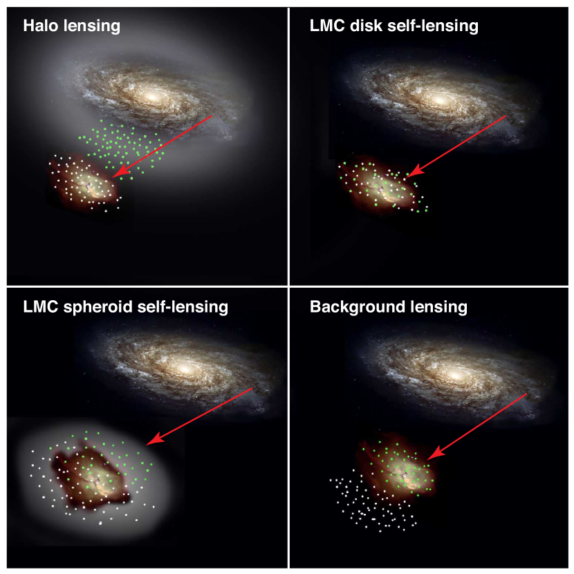
Figure 1: Possible LMC microlensing geometries. The Milky Way is depicted as the large spiral galaxy in the upper right hand corner, the LMC as the irregular galaxy in the lower left hand corner. In each figure the arrow indicates a line of sight from the location of the Earth in the Milky Way towards a random position in the LMC. The white dots indicate the position of the source stars, the green dots the position of the lenses. Figure not to scale.

Each of the above LMC microlensing geometries is depicted pictorially in Figure 1.

A final possibility is foreground self-lensing. This is not self-lensing in the classical sense as in this case the lenses are not drawn from the LMC itself, but rather from some kinematically distinct foreground population, such as an intervening dwarf galaxy. Zaritsky & Lin (1997) claim a detection of a population of stars from such an entity. However, Beaulieu & Sackett (1998) claim that this population is a morphological feature of the LMC red clump, while others show that such a population consistent with other observational constraints could not produce a substantial microlensing signal (Gould, 1998; Bennett, 1998). Zaritsky et al. (1999) argue that may be possible to evade these constraints by tuning the IMF of this putative foreground population. But the a priori probability for such a large mass of stars to exist in the foreground of the LMC is already quite low, so this explanation seems rather unlikely. We do not consider this model any further.

3 WFPC2 Observations of Microlensing Source Stars

Observations were made under proposals GO-05901, GO-7306 and GO-8676 (Principal Investigator: Kem Cook) with the WFPC2 on the HST between May 1997 and July 2000 through the F555W ($V$) and F814W ($I$) filters. The Planetary Camera (PC) was centered on the location of past MACHO microlensing events. The microlensing events, positions, and exposure times are listed in Table 1.

Multiple exposures of a field were combined using a sigma-clipping algorithm to remove deviant pixels, usually cosmic rays. The PC has a pixel size of 0$\buildrel\prime\prime\over{.}$046 which easily resolves the great majority of stars in our frames. Most stars are also resolved in the Wide Field (WF) fields which have a pixel size of 0$\buildrel\prime\prime\over{.}$1. Instrumental magnitudes were calculated from aperture photometry using DAOPHOT II (Stetson, 1987, 1991) with a radius of 0$\buildrel\prime\prime\over{.}$25 and centroids derived from point-spread function (PSF) fitting photometry. Aperture corrections to 0$\buildrel\prime\prime\over{.}$5 were performed individually for each frame. We choose this aperture radius as this is how the Holtzman et al. (1995) calibrations are defined. We correct for the WFPC2 charge transfer effect using the equations from Instrument Science Report WFPC2 97-08. We also make the minimal corrections for contaminants which adhere to the cold CCD window according to Table 28.2 of the HST Data Handbook. We transform our instrumental magnitudes to Landolt $V$ and $I$ using the calibrations from Holtzman et al. (1995).

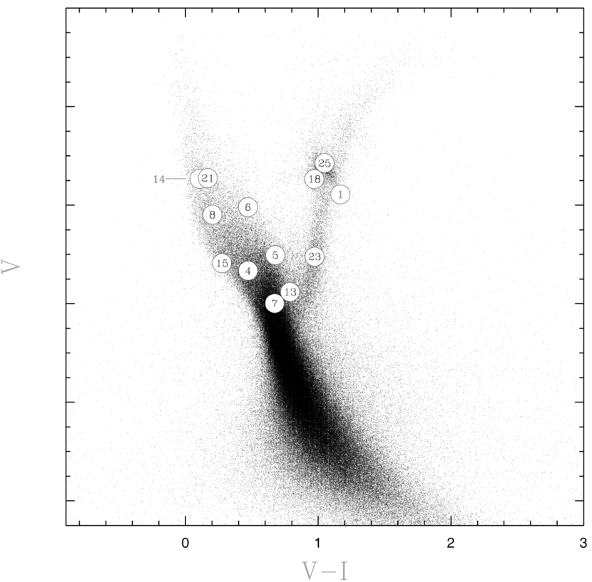
Figure 2: Color magnitude diagram of LMC microlensed source stars. The source stars are overplotted on a composite HST CMD of the fields surrounding each of these events. The numbers indicate the corresponding MACHO microlensing event.

We create a composite LMC CMD by combining the PC and WF photometry for all of our fields except the field of LMC-1. In the case of LMC-1 the $V$ and $I$ observations were taken at different roll angles and there is little area of overlap except in the PC frame. We therefore include the PC field from LMC-1 but not the WF fields. The composite HST CMD is shown in Figure 2.

4 Source Star Identification

A ground-based MACHO image has a pixel size of 0$\buildrel\prime\prime\over{.}$6 and a seeing of at least 1$\buildrel\prime\prime\over{.}$4. In a typically crowded region of the outer LMC bar, a MACHO seeing disk will contain $\sim$11 stars of $V\lesssim 24$. This means that faint “stars” in ground-based MACHO photometry are usually not single stars at all, but rather blended composite objects made up of several fainter stars. Henceforth, we distinguish between these two words carefully, using object to denote a collection of stars blended into one seeing disk, and star to denote a single star, resolved in an HST image or through difference image analysis. The characteristics of the MACHO object that was lensed tell us little about the actual lensed star. However, with the microlensing object centroid from the MACHO images we can hope to identify the microlensing source star in the corresponding HST frame.

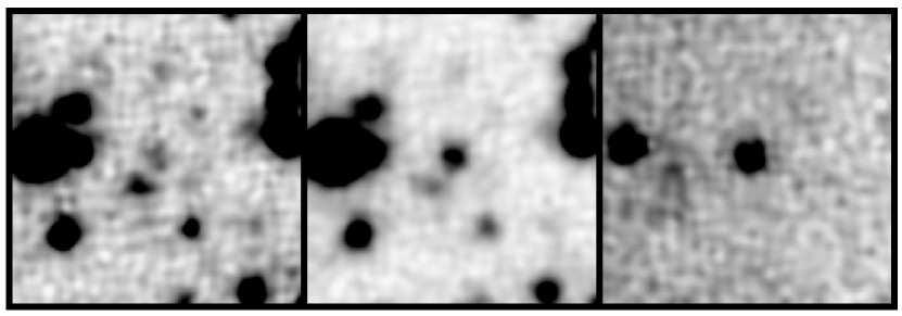
Figure 3: Difference Image Analysis. The left panel shows a $0.6^{\prime}~{}\times~{}0.6^{\prime}$ section of the baseline image of MACHO event LMC-4. The middle panel shows the same region taken at the peak of the microlensing event. The right panel shows the differenced image. The flux in the middle of the differenced image is the extra flux from the microlensing event. The flux at the left hand side of the differenced image is an expected contamination due to an asymptotic giant branch variable star at that location.

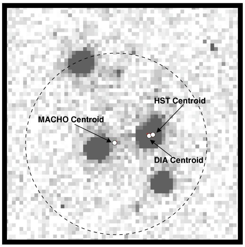
Figure 4: DIA results for event LMC-4. A $3^{\prime\prime}~{}\times~{}3^{\prime\prime}$ HST image of LMC-4. The circle contains the several HST stars which are all contained within one MACHO seeing disk of the lensed object. The arrows indicate the MACHO baseline centroid, the DIA centroid and the centroid of the HST star nearest to the DIA centroid.

A direct coordinate transformation from the MACHO frame to the HST frame often places the baseline MACHO object centroid in the middle of a group of faint HST stars with no single star clearly identified. To resolve this ambiguity we have used DIA. This technique is described in detail by Tomaney & Crotts (1996) and Alcock et al. (1999b), but we review the main points here. DIA is an image subtraction technique designed to provide accurate photometry and centroids of variable stars in crowded fields. The basic idea is to subtract a flux and seeing matched high S/N reference image from each from each program image, leaving a differenced image containing only the variable components. Applied to microlensing, we subtract baseline images from images taken at the peak of the microlensing light curve, leaving a differenced image containing only the flux from the microlensing source star and not the rest of the object. We typically observe a centroid shift between the MACHO object’s location and the residual lensed flux in the difference image. If the centroid from the differenced image is transformed to the HST frame we find that it usually clearly identifies the HST microlensed source star. This process is illustrated in Figures 3 and 4.

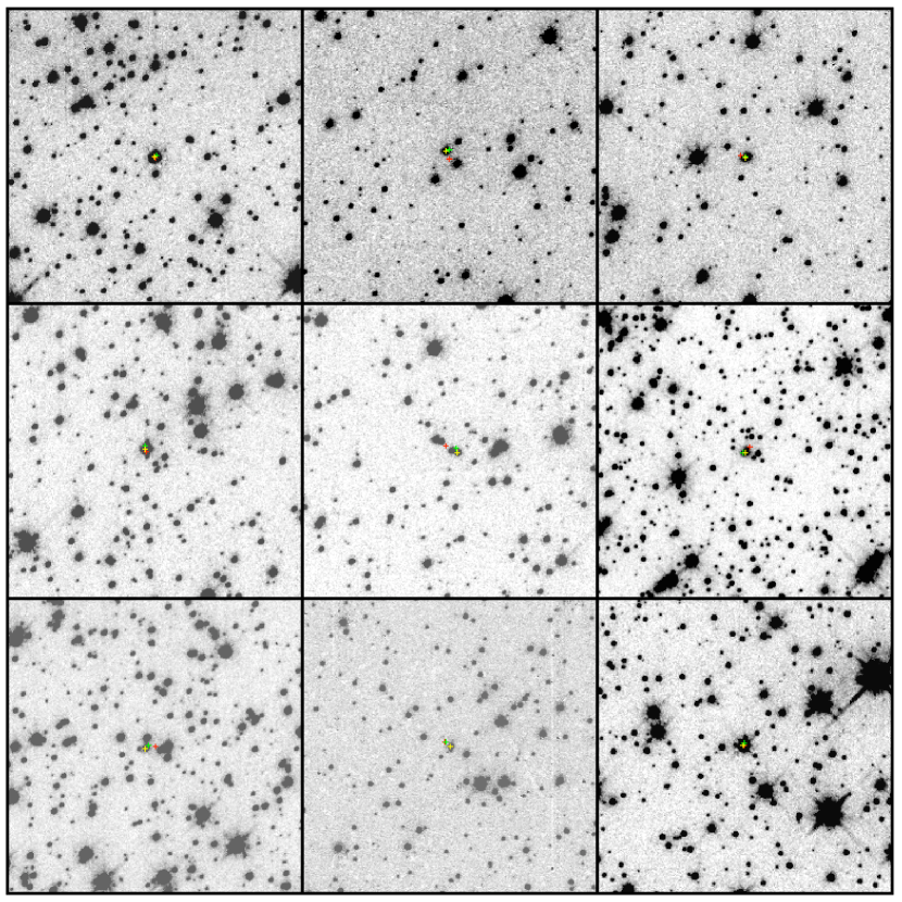
Figure 5: HST finding charts for microlensing source stars I. From top to bottom, left to right, we show LMC-1, LMC-4, LMC-5, LMC-6, LMC-7, LMC-8, LMC-9, LMC-13, and LMC-14. The MACHO object centroid is shown as a red cross, the DIA centroid is shown as a green cross and the centroid of the HST star closest to the DIA centroid is shown as a yellow cross.

In Figures 5 and 6 we present WFPC2 finding charts identifying the MACHO object centroid, the centroid in the DIA image and the centroid of the star in the WFPC2 image closest to the DIA centroid.

This technique allows us to unambiguously identify the 13 microlensed source stars which pass the cut A microlensing tests in Alcock et al. (2000b). In Table 2 we present the $V$, $R$, and $I$ magnitudes of our source stars from the HST data. The errors presented here include the formal photon counting errors returned by DAOPHOT II as well as an additional $0.03$ mag uncertainty due to aperture corrections. We note that the cut A microlensing events do not include LMC-9 (which appeared in a similar analysis by Alcock et al. (2001c)). Although LMC-9 is certainly a valid microlensing event, it is a binary microlensing event (Bennett et al., 1996) and therefore its non-standard light curve does not pass the stringent cut A requirements. Although we list its photometric information in Table 2, it is not used in our statistical analysis.

Our identification of LMC-5 revealed it to be the rather rare case of a somewhat blended HST star (Alcock et al., 2001e). Although there are two stars evident, at an aperture of 0$\buildrel\prime\prime\over{.}$25 the flux of one star was contaminated by that of its neighbor. Therefore, in this case, we perform PSF fitting photometry using PSFs kindly provided by Peter Stetson. The errors presented in Table 2 for LMC-5 are those returned by the profile fitting routine ALLSTAR. The DIA centroid falls 2 pixels closer to the centroid of star one than star two, clearly preferring star one as the source star. Furthermore, as predicted by Alcock et al. (1997) and Gould, Bahcall, & Flynn (1997), star two is a rather red object which is very faint in the V band. Fits to the MACHO light curve presented by Alcock et al. (2000b) suggest lensed flux fractions in the V and R bands of 1.00 and 0.46 respectively, confirming the DIA choice of the much bluer star as the lensed source star. In addition to these HST/WFPC2 observations Alcock et al. (2001e), a second epoch of HST observations using the Advanced Camera for Surveys (ACS) were obtained (Drake et al., 2004), and these data combined with a microlensing parallax analysis (Gould, 2004) resulted in the first stellar mass measurement of a single star besides the Sun (Gould, Bennett, & Alves, 2004). The LMC-5 lens star has a mass of $0.097\pm 0.016M_{\odot}$.

An important source of background for microlensing events in these crowded fields is due to distant galaxies behind the LMC. This was first noticed in Alcock et al. (1997), where event LMC-11 was seen to be very close to an obvious background spiral galaxy. This and the asymmetric light curve indicated that the variability was almost certainly due to a background supernova and not microlensing. Background supernovae were considered in some detail in Alcock et al. (2000b), where a detailed supernova rejection procedure was developed. Events were rejected if

1. a supernova type Ia model provided a better fit than microlensing, or

2. a background galaxy was visible in the proximity of the event.

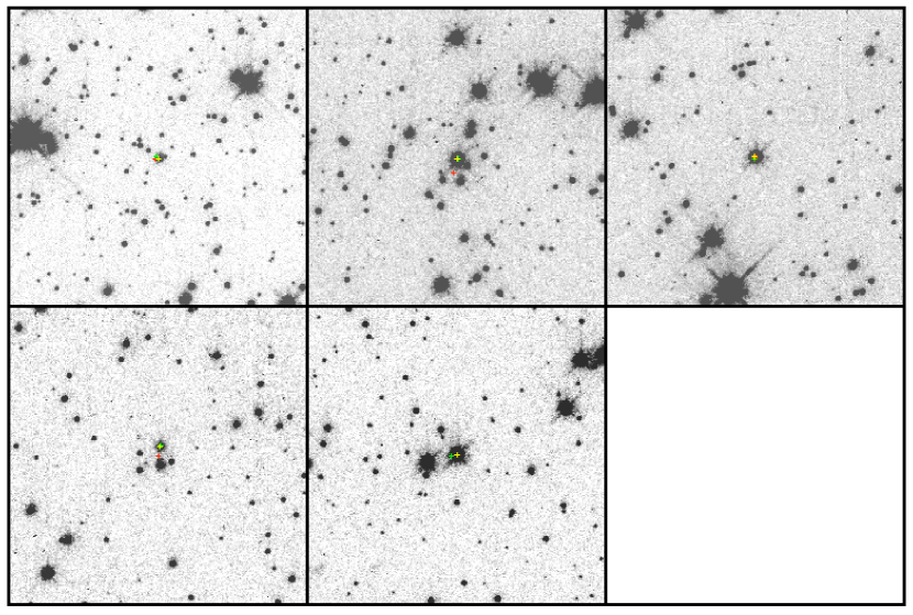
Figure 6: HST finding charts for microlensing source stars II. As in Figure 5 for events LMC-15, LMC-18, LMC-21, LMC-23, and LMC-25.

This procedure is expected to work because the type II supernovae with light curves that don’t resemble type Ia light curves are generally associated with galaxies that are closer and have more young stars, so that they should be visible in the MACHO images. This procedure seems to remove all the supernovae contamination from the MACHO sample, but there are a few events, such as LMC-10 and 22, for which host galaxy is so compact that it looks like a star in the MACHO images. Thus, an important check of our background rejection procedure is that all of the events should not be associated with background galaxies. A careful inspection of the HST images (see Figs. 5 and 6) reveals no extended sources in the vicinity of the lens events, so the efficiency of our supernovae rejection method is confirmed.

5 Comparison with MACHO Blend Fits

As discussed above, in a ground-based MACHO image each microlensed “star” is often a blended composite image of several fainter stars. Only one of the stars which make up the composite object is microlensed. In this section, we have described one method for identifying the microlensed star in the WFPC2 image.

However, there exists another method for estimating the percentage of the total object flux which was actually microlensed. The ground-based object flux may separated into lensed and unlensed components by performing a microlensing blend fit to the ground-based lightcurve. This procedure is described in detail by Alcock et al. (1997) and Alcock et al. (2000b).

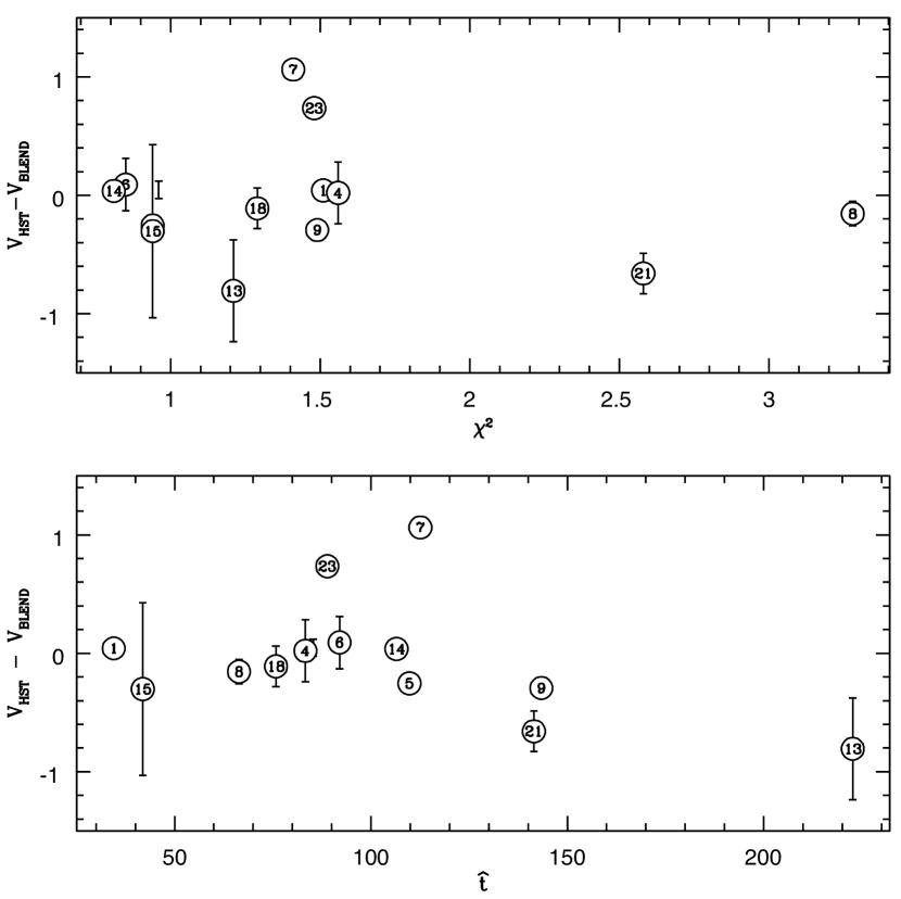
Figure 7: A comparison between the HST source star magnitude, $V_{\rm HST}$ and the estimated source star magnitude derived from a microlensing blend fit to the ground-based lightcurve, $V_{\rm blend}$. We plot the difference versus the event-duration, $\hat{t}$ and the reduced chi-squared of the fit, $\chi^{2}$. We show error bars only when they are larger than the dots.

In Table 2, we calibrate the lensed flux for each event as presented in Table 5 of Alcock et al. (2000b). The calibrated lensed flux is an estimate of the source star (not object) magnitude, derived entirely from the ground-based photometry. Thus, we would expect $V_{\rm HST}\sim V_{\rm blend}$ and $R_{\rm HST}\sim R_{\rm blend}$. We show a plot of the difference $V_{\rm HST}-V_{\rm blend}$ in Figure 7. We plot the difference versus the event duration, $\hat{t}$ and the reduced chi-squared of the microlensing blend fit (see Table 5 of Alcock et al. (2000b)).

The blend fits work reasonably well for all events except LMC-7, LMC-13, LMC-21 and LMC-23. The case of LMC-13 is considered by Bennett et al. (2005), who show that the blend fit is consistent with the source identified in the HST frames when follow-up CTIO photometry and improved DIA photometry of the MACHO survey data is used in the fits. For LMC-21, the blend fits indicate a source that is $\sim 0.7$ mag fainter than the corresponding source in the HST frames, but the $R-V$ colors of the blend fit sources and the HST image are equal to within their errors. Thus, this event might be explained if the source has a binary companion of almost equal brightness at a separation larger than a few AU.

For LMC-7, the blend fit source also has a color that is similar to the color seen in the HST images, but in this case the blend fit source is brighter. So, this cannot be explained by a source companion. The light curve is symmetric and achromatic, with a peak magnification of 6.9, but it also has significant deviations from the standard, single lens microlensing light curve. This could be caused by a non-standard microlensing effect, such as a weak binary lens, microlensing parallax (Gould, 1992; Alcock et al., 1995) or xallarap (Griest & Hu, 1992; Poindexter et al., 2005), which is the result of orbital motion of the source (i.e.parallax reversed). The HST star for this event does appear to be slightly redder than the blend fit source. If this does not reflect photometry problems (as was the case with LMC-13), it might indicate a very red foreground Milky Way disk lens as was the case for events LMC-5 (Alcock et al., 2001e) and LMC-20 (Kallivayalil et al., 2006). (LMC-20 is a lower S/N microlensing event that did not pass all the sample A cuts.) If this excess red flux is really from the source, then there is a very good chance that the light curve will show a parallax deviation.

LMC-23 is the one source that shows a large color offset between the blend fits and the HST photometry, with the HST blend fits indicating a source about 0.3 mag bluer than the HST frame. This event also has significant light curve deviations that can probably not be explained by a reasonable microlensing model (Bennett et al., 2005). In fact, data from the EROS (Tisserand et al., 2007) and OGLE (Udalski, 2004, private communication) groups show an additional brightening that occurred after the MACHO survey stopped taking data. It is possible, but unlikely, for binary source or binary lens model to produce two light curve bumps separated by a year or more (Alcock et al., 2000a), but it is virtually impossible to also ascribe the poor microlensing fit to non-standard microlensing. The only reasonable conclusion is that this event is not microlensing, but is actually due to a variable star. However, this is the only MACHO LMC event that has been confirmed to be something besides a microlensing event, and a careful analysis of all the MACHO LMC events indicates that contamination of the MACHO sample by non-microlensing variability leads to only a small correction to the microlensing optical depth (Bennett, 2005).

6 Creation of Model Source Star Populations

We consider source stars drawn from two distinct populations: the disk+bar of the LMC and a background population located behind the LMC disk. Source stars from the disk+bar of the LMC are well represented by our composite HST CMD shown in Figure 2. Source stars drawn from the background population will be on average redder than the disk+bar by an amount equal to the mean extinction through the LMC and may also be displaced behind the LMC by some distance.

The mean internal extinction of the LMC has been determined using UBV and UBVI photometry of young, hot (O–A type) stars in Oestricher & Schmidt-Kaler (1996) and Harris, Zaritsky & Thompson (1997). Oestricher & Schmidt-Kaler (1996) find a mean internal reddening due to dust in the LMC disk of $\overline{E(B-V)}=0.16$ and Harris, Zaritsky & Thompson (1997) find $\overline{E(B-V)}=0.13$.

A more recent study (Zaritsky, 1999) suggests that the reddening of the LMC may be population dependent. Zaritsky (1999) find $\overline{E(B-V)}=0.17$ for hot, young stars ($T>22,000$ K), but a much lower internal reddening for older, cooler stars ($5500~{}K<T<6500~{}K$) of $\overline{E(B-V)}=0.03$. The lower reddening for older stars may be due to the difference in scale heights of an old population and a young population relative to the scale height of the dust (i.e., the old population may have a larger scale height) combined with the presence of low-extinction “holes” in the dust layer. In this interpretation, the large scale height of old stars implies that about half the cool stars live in front of the LMC dust plane and are only extincted by Galactic foreground dust. In contrast, the small scale height of the young stars implies that the majority live within the dust plane and suffer from both foreground and internal extinction. Of the stars lying behind the LMC midplane, some fraction are found in “holes” and are again only extincted by the Galactic foreground dust. According to Zaritsky (1999) such a model works well in predicting both the hot star and cold star extinctions in the LMC.

If the above interpretation of population dependent reddening is correct, then the mean reddening for the young hot stars is an appropriate measure of the total internal reddening of the LMC disk. However, the concept of a patchy LMC extinction is problematic for our Kolmogorov-Smirnov test in which we assume that the reddening of all of our fields is approximately the same. Empirically, we find that the reddening of our fields is approximately the same. If we shift our CMDs up and down the reddening axis until they seem to line up perfectly (by eye), we find that the maximum shift is within $\Delta E(B-V)\sim 0.03$ of the mean.

The high reddenings for young, hot stars may also be due to environmental effects, e.g., the young stars may still live very close to the dust in which they were formed. In this case, the young star reddening may significantly overestimate the true mean internal reddening of the LMC disk.

In this work, we adopt the same value as used in Zhao, Graff & Guhathakurta (2000), $\overline{E(B-V)}=0.13$. This is the lowest mean value determined using young stars, but is significantly higher than the Zaritsky (1999) value for old stars. We note, that if the true value is significantly lower than $\overline{E(B-V)}=0.13$, the statistical significance of our Kolmogorov-Smirnov test would decrease substantially.

The distance to the background population of $\Delta\mu\sim 0.3$ from Zhao, Graff & Guhathakurta (2000) is very loosely derived by the requirement that the background population be at least transiently gravitationally bound to the LMC. We consider three different displacement distances from $\Delta\mu=0.0$, $\Delta\mu=0.3$ ($\sim 7.5$ kpc) and $\Delta\mu=0.45$ ($\sim 11.5$ kpc). We have no constraints on the location, size or content of a possible background population, except that it must be small enough and similar enough to the LMC stellar population to have avoided direct detection.

For each model source star population we begin with the composite HST CMD and then shift some fraction, $f_{\rm BKG}$, of the stars into the background. That is, we redden and displace a fraction $f_{\rm BKG}$ of the CMD by amounts

$$\Delta V=A_{V}+\Delta\mu~{},$$ (1)

$$\Delta(V-I)=E(V-I)=1.376\cdot E(B-V)=0.18~{}{\rm mag}.$$ (2)

The coefficient in the conversion from $E(B-V)$ to $E(V-I)$ is drawn from Table 6 of Schlegel, Finkbeiner & Davis (1998) and $A_{V}=3.315\cdot E(B-V)=0.43$ mag. We use the Landolt coefficients from Schlegel, Finkbeiner & Davis (1998) since the Holtzman et al. (1995) coefficients calibrate the WFPC2 magnitudes to this system.

Each CMD now contains a fraction $1.0-f_{\rm BKG}$ source stars from the LMC disk+bar and a fraction $f_{\rm BKG}$ of source stars from the background population. The CMD now represents the distribution of source stars down to $V\sim 24$. However, not all possible microlensing events are detected in the MACHO images. To create a CMD representing a population of source stars which produce detectable microlensing events we must convolve the HST CMD with the MACHO detection efficiency. The MACHO efficiency pipeline is extensively described by Alcock et al. (2000b) and Alcock et al. (2001d) and the detection efficiency as a function of stellar magnitude, $V_{\rm{star}}$, and Einstein ring crossing time has been calculated. We average this function over the event durations of the thirteen events from Alcock et al. (2000b) and present the MACHO detection efficiency as a function of $V_{\rm{star}}$ in Figure 8. We convolve this function with our HST CMDs to produce the final model source star CMDs.

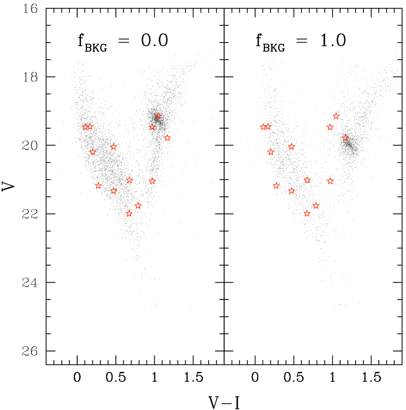
Figure 9: We show the observed microlensing source stars as large red stars, overplotted on two model source star populations (small black dots). The left hand panel represents a source star population drawn entirely from the LMC disk+bar ($f_{\rm BKG}=0.0$). The right hand panel represents a model in which all of the stars belong to a background population ($f_{\rm BKG}=1.0$) with $\Delta\mu=0.3$ and $\Delta E(V-I)=0.18$.

In Figure 9, we illustrate two model source star populations, both with $\Delta\mu=0.30$, one with $f_{\rm BKG}=0.0$ (all source stars in the LMC disk+bar) and one with $f_{\rm BKG}=1.0$ and $\Delta\mu=0.30$ (all source stars in a background population displaced by 7.5 kpc). We overplot the observed microlensing source stars of Table 2 as large red stars.

This procedure is based on several assumptions. First, we assume that our thirteen HST fields collectively well represent the stellar population of the LMC disk. This assumption has two parts, the first being that an observation at a random line of sight in the LMC bar is dominated by stars in the LMC disk and the second that the stellar population across the LMC is fairly constant. The first part holds so long as the surface density of the background population is much smaller than that of the LMC itself. If this were not the case, this population would have been directly detected. The second part has been confirmed by many LMC population studies including Alcock et al. (2001d), Olsen (1999), and Geha et al. (1998), as well as our own comparison of individual CMDs and luminosity functions. In addition, as mentioned above, we find that all of our fields have reddenings within about $\Delta E(B-V)\sim 0.03$ of their mean value.

7 Statistical Method and Results

We now determine which model source star population is most consistent with the observed CMD of microlensed source stars by performing a two-dimensional Kolmogorov-Smirnov test.

In the familiar one dimensional case, a KS test of two samples with number of points $N_{1}$ and $N_{2}$ returns a distance statistic $D$, defined to be the maximum distance between the cumulative probability functions at any ordinate. Associated with $D$ is a corresponding probability $P(D)$ that if two random samples of size $N_{1}$ and $N_{2}$ are drawn from the same distribution a worse value of $D$ will result. This is equivalent to saying that we can exclude the hypothesis that the two samples are drawn from the same distribution at a confidence level of $1.0-P(D)$. If $N_{2}\gg N_{1}$, then this is also equivalent to excluding at a $1.0-P(D)$ confidence level the hypothesis that sample 1 is drawn from sample 2.

The concept of a cumulative distribution is not defined in more than one dimension. However, it has been shown that a good substitute in two dimensions is the integrated probability in each of four right-angled quadrants surrounding a given point (Fasano & Franceschini 1987; Peacock 1983). That is, consider a point $(x_{1},y_{1})$ in distribution $N_{1}$ and draw two perpendicular lines through this point (one line perpendicular to the $x$ axis and the other perpendicular to the $y$ axis) which divide the space into four quadrants. The integrated probability of each quadrant for each distribution is the fraction of data from the distribution which lies in that quadrant. The two dimensional KS statistic $D$ is now taken to be the maximum difference (ranging both over all data points and all quadrants) between the integrated probability of distribution $N_{1}$ and $N_{2}$. See Press et al. (1992) for further details. The distance statistic $D$ and the corresponding $P(D)$ are subject to the same interpretation as in the one dimensional case.

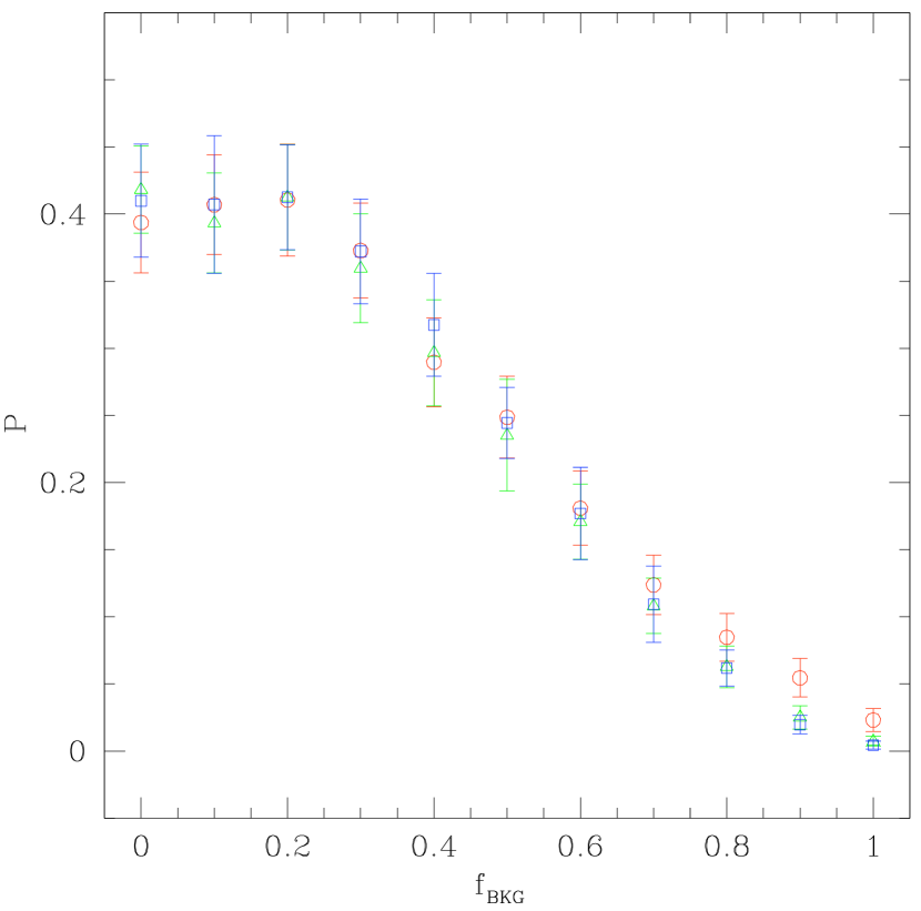
Figure 10: Kolmogorov-Smirnov test results. The 2-D KS test probability $P$ that our observed distribution of source stars was drawn from a source star population in which a fraction $f_{BKG}$ of the source stars are located behind the LMC. The distance moduli of the background stars with $\Delta\mu=0.0,0.30,0.45$ are shown as red circles, green triangles and blue squares respectively. The errors bars indicate the scatter about the mean value for 20 simulations of each model.

We show the resulting $P(D)$ plotted versus $f_{\rm BKG}$ in Figure 10. The results are shown separately for $\Delta\mu=0.0,0.3$ and $0.45$ in red circles, green triangles, and blue squares, respectively. The error bars indicate the scatter about the mean value for 20 simulations of each model. Because the creation of the efficiency convolved CMD is a weighted random draw from the HST CMD, the model population created in each simulation differs slightly. This in turn leads to small differences in the KS statistics. We find that the 2-D KS-test probability is highest at a fraction of source stars behind the LMC $f_{\rm BKG}~{}\sim 0.0-0.2$ with very little dependence on the value of the displacement, $\Delta\mu$. The significant preference for low $f_{\rm BKG}$ arises mostly from reddening/color.

In a strict statistical sense, the KS test can only be used to reject or confirm the hypothesis that two datasets have a common parent distribution. As a general guideline, a probability of less than 10% suggests that the two distributions are significantly different (Press et al. 1992). It is not strictly allowable to compare relative probability, e.g., a KS test probability of 80% does not mean that it is twice as likely that two distributions are identical than if they had returned a KS test probability of 40%. However, we still find it valuable to show the shape of our KS test probability function to demonstrate its insensitivity to $\Delta\mu$.

8 Discussion

We now compare the observational results for $f_{\rm BKG}$ (Figure 10) with the expected value for our four models of microlensing: a) background lensing ($f_{\rm BKG}\sim 1.0$), b) LMC spheroid self-lensing ($f_{\rm BKG}\lower 2.15277pt\hbox{$\;\buildrel<\over{\sim}\;$}0.65$), c) LMC disk+bar self-lensing ($f_{\rm BKG}\sim 0.0$), and d) MW lensing ($f_{\rm BKG}\sim 0.0$).

We rule out a model in which the source stars all belong to some background population at a confidence level of $99$% (e.g., the KS test probability for $f_{\rm BKG}=1.0$ is $<0.01$). Of course, one event of this sample, LMC-5, is known to be caused by a lens in the Milky Way disk, but $f_{\rm BKG}=0.9$ and $f_{\rm BKG}=0.8$ are excluded by $>95\,$% and $>90\,$%, respectively. So, background source models would seem to be excluded. But, this conclusion might be weakened if we had allowed for patchy extinction within the LMC.

We can rule out spheroid self-lensing models where the spheroid has the same luminosity function as the disk+bar ($f_{BKG}\sim 0.65$) at the statistically marginal confidence level of $80-90$%. But old spheroid self-lensing models without A and F stars in the spheroid have $f_{BKG}<0.65$ and are not significantly disfavored by this analysis. The relatively low number density of LMC halo RR Lyrae (Minniti et al., 2003) suggests that the LMC spheroid microlensing optical depth should be quite low, but there are several reasons not to dismiss the LMC spheroid self-lensing models. First, as Weinberg (2000) emphasized, the LMC is not an isolated galaxy, and the interactions of the LMC with the Milky Way and the Small Magellanic Could (SMC) significantly complicate attempts to properly model its structure. Thus, the lack of an LMC model that provides a sufficient microlensing optical depth while fitting the other observational constraints may just reflect our failure to model the MW + LMC + SMC system.

The allowed region of the $f_{\rm BKG}$ plot ($P>10$%) is consistent with the expected location of the source stars in both the MW-lensing and LMC disk+bar self-lensing geometries. However, detailed modelling of LMC disk+bar self-lensing suggests that it contributes only 25% of the observed optical depth (Gyuk, Dalal, & Griest, 2000; Mancini et al., 2004). So, the test presented here seems most consistent with having the majority of events located in the MW halo, with some contribution from the LMC disk+bar and MW disk.

There are, however, additional reasons that favor the LMC spheroid self-lensing model. The strongest point in favor of LMC spheroid self-lensing is the apparent spacial distribution of the LMC microlensing optical depth. While the spacial distribution of the MACHO events does not match expectations from LMC disk+bar self-lensing (Mancini et al., 2004), LMC spheroid self-lensing should produce a much more uniform distribution of events across the central regions of the LMC where the MACHO survey had high sensitivity (within $\lower 2.15277pt\hbox{$\;\buildrel<\over{\sim}\;$}3^{\circ}$ of the LMC-bar center). However, the EROS survey has very low sensitivity to microlensing in this central part of the LMC, as most of their sensitivity comes from fields that are $\lower 2.15277pt\hbox{$\;\buildrel>\over{\sim}\;$}3^{\circ}$ from the center of the LMC-bar. Since LMC spheroid self-lensing should provide a much lower optical depth in these outer fields, it would seem that LMC spheroid self-lensing might provide a reasonable explanation for both the MACHO and EROS results.

Some of the handful of Magellanic Cloud microlensing events with distance estimates also provide some clues to the locations of the other lenses. LMC-5 and LMC-20 (from the B sample of Alcock et al. (2000b)) have both been confirmed to be MW disk lenses (Alcock et al., 2001e; Kallivayalil et al., 2006), but they have been detected by methods that can only detect lenses that are close to us, so they don’t really inform us about the location of other events. The situation is similar for the binary source event, LMC-14, which has been shown to be caused by a lens in the LMC disk+bar or spheroid (Alcock et al., 2001b). The binary source effects that lead to this conclusion are only detectable for lenses that reside in the LMC, some self-lensing events are expected for any reasonable model of the LMC. On the other hand, only a minority of self-lensing events should show this effect, so one might argue that such an event should be accompanied by a number of other self-lensing events that don’t show this effect. But this argument doesn’t have much statistical significance since it is based on only a single event.

It is more informative to consider events that can reveal distance information no matter where the lens resides. There are two types of such events: binary lens events with resolved caustic crossings, and events with space-based microlensing parallax measurements. Event LMC-9 is a binary lens event with a caustic crossing that is marginally resolved by only two measurements (Bennett et al., 1996). The long caustic crossing time favors a LMC disk+bar lens, but due to the poor sampling of the caustic crossing alternative interpretations are possible. Event MACHO-98-SMC-1 was announced by the MACHO Alert system (Alcock et al., 1996, 1999a) prior to the second caustic crossing, which enabled the EROS, MPS, OGLE and PLANET collaborations to join MACHO in monitoring the event. This allowed the second caustic crossing to be well resolved, and the observed caustic crossing timescale indicated that the lens resided in the SMC (Afonso et al., 2000). However, the SMC is known to be much more extended along the line-of-sight than the LMC, so its self-lensing optical depth is expected to be much larger. So, the fact that this lens is likely to be in the SMC does not imply that most LMC sources have lenses that are also in the LMC.

The situation with the only event (OGLE-2005-SMC-1) with a space-based microlensing parallax measurement (Dong et al., 2007) is somewhat more interesting because the analysis favors a MW halo lens over a lens in the SMC by a 20:1 likelihood ratio. However, if the lens is in the MW halo, then it is almost certainly more massive than the lenses for the LMC microlensing events found by MACHO. So, it doesn’t really support the MW halo model for the LMC lenses, either. However, it does seem plausible that this event could be explained by a SMC-spheroid lensing population that is larger than predicted by standard SMC models.

9 Summary

We have presented HST follow-up observations of 13 LMC microlensing events presented in Alcock et al. (2000b) including the 12 genuine microlensing events passing the cuts for for selection criteria A. These HST data support our conclusions, based on light curve modeling, that these are genuine microlensing events, and they also strengthen the conclusion that the MACHO LMC microlensing sample does not have significant contamination due to non-microlensing variability.

We have also compared the colors and magnitudes of our source stars to the predictions of various models to determine which models of LMC microlensing might be consistent with the observed events. At present, the strength of this analysis is severely limited by the number of microlensing events. We are currently able to exclude the most extreme model ($f_{\rm BKG}\sim 1.0$), but with more events, it should be possible to more accurately determine $f_{\rm BKG}$ and judge intermediate models such as LMC spheroid or shroud self-lensing. Ongoing microlensing search projects (OGLE-III, MOA-II, SuperMACHO) may supply a sufficient sample of events in the next few years. The technique outlined in this paper should prove a powerful method for locating the sources, and, subsequently, the lenses with these future datasets.

At present, there exist no theoretical models that adequately explain the microlensing optical depth seen towards the LMC. LMC spheroid or shroud models seem most likely to fit the spacial distribution of microlensing events seen in the combined MACHO plus EROS data sets.

Figure 8: The MACHO detection efficiency as a function of stellar V-magnitude. If a microlensing event occurs in a star of given magnitude $V_{star}$, this is the given efficiency for detecting that event.

.

Table 1: WFPC2 Observations of Microlensing Source Stars

Event	RA	DEC	V	R	I	Obs Date
LMC-1	05:14:44.53	$-$68:47:56.31	$4~{}\times~{}400$	$4~{}\times 400$	$40~{}\times~{}400$	1997/12/16
LMC-4	05:17:14.59	$-$70:46:55.28	$3~{}\times~{}500$	$3~{}\times 500$	$33~{}\times~{}500$	1997/12/12
LMC-5	05:16:41.22	$-$70:29:21.22	$4~{}\times~{}400$	$2~{}\times 400$	$2~{}\times~{}400$	1999/05/13
LMC-6	05:26:13.77	$-$70:21:16.37	$4~{}\times~{}400$	$2~{}\times 400$	$2~{}\times~{}400$	1999/08/26
LMC-7	05:04:03.61	$-$69:33:21.00	$4~{}\times~{}400$	$2~{}\times 400$	$2~{}\times~{}400$	1999/04/12
LMC-8	05:25:09.65	$-$69:47:53.82	$4~{}\times~{}400$	$2~{}\times 400$	$2~{}\times~{}400$	1999/03/12
LMC-9	05:20:20.52	$-$69:15:13.84	$4~{}\times~{}400$	$2~{}\times 400$	$2~{}\times~{}400$	1999/04/13
LMC-13	05:24:02.83	$-$68:49:14.77	$3~{}\times~{}500$	$3~{}\times 500$	$3~{}\times~{}500$	2000/07/28
LMC-14	05:34:44.54	$-$70:25:10.09	$4~{}\times~{}500$	$2~{}\times 400$	$4`\times~{}500$	1997/05/13
LMC-15	05:05:45.86	$-$69:43:54.02	$3~{}\times~{}500$	$3~{}\times 500$	$3~{}\times~{}500$	2000/07/17
LMC-18	05:45:20.87	$-$71:09:15.20	$3~{}\times~{}500$	$3~{}\times 500$	$3~{}\times~{}500$	2000/07/21
LMC-20	04:54:18.81	$-$70:02:21.39	$3~{}\times~{}500$	$3~{}\times 500$	$3~{}\times~{}500$	2000/07/29
LMC-21	04:57:13.82	$-$69:27:50.57	$3~{}\times~{}500$	$3~{}\times 500$	$3~{}\times~{}500$	2000/07/26
LMC-23	05:06:16.85	$-$70:58:49.98	$3~{}\times~{}500$	$3~{}\times 500$	$3~{}\times~{}500$	2000/07/18
LMC-25	05:02:15.86	$-$68:00:55.10	$3~{}\times~{}500$	$3~{}\times 500$	$3~{}\times~{}500$	2000/07/14

Note. — The columns V and I indicate the number of single exposures times the number of seconds per exposure.

Table 2: WFPC2 and MACHO Blend Fit Photometry of Microlensing Source Stars

Event	$V_{\rm HST}$	$R_{\rm HST}$	$I_{\rm HST}$	$V_{\rm blend}$	$R_{\rm blend}$	$\chi^{2}$
LMC-1	$19.78\pm 0.03$	$19.20\pm 0.03$	$18.61\pm 0.03$	$19.74\pm 0.02$	$19.19\pm 0.02$	1.510
LMC-4	$21.33\pm 0.03$	$21.09\pm 0.03$	$20.83\pm 0.03$	$21.31\pm 0.26$	$21.08\pm 0.26$	1.560
LMC-5	$21.02\pm 0.07$	$20.72\pm 0.07$	$20.34\pm 0.08$	$21.27\pm 0.02$	$21.01\pm 0.03$	0.940
LMC-6	$20.04\pm 0.03$	$19.86\pm 0.03$	$19.57\pm 0.03$	$19.95\pm 0.22$	$19.82\pm 0.23$	0.850
LMC-7	$21.99\pm 0.03$	$21.76\pm 0.04$	$21.32\pm 0.03$	$20.93\pm 0.02$	$20.83\pm 0.03$	1.410
LMC-8	$20.20\pm 0.03$	$20.18\pm 0.03$	$19.99\pm 0.03$	$20.35\pm 0.10$	$20.09\pm 0.10$	3.280
LMC-9∗	$21.14\pm 0.03$	$20.65\pm 0.03$	$20.15\pm 0.03$	$21.43\pm 0.02$	$20.88\pm 0.02$	1.490
LMC-13	$21.76\pm 0.03$	$21.38\pm 0.03$	$20.92\pm 0.03$	$22.57\pm 0.43$	$22.11\pm 0.43$	1.210
LMC-14	$19.47\pm 0.03$	$19.46\pm 0.03$	$19.36\pm 0.03$	$19.43\pm 0.08$	$19.46\pm 0.08$	0.810
LMC-15	$21.18\pm 0.03$	$21.07\pm 0.03$	$20.90\pm 0.03$	$21.48\pm 0.73$	$21.37\pm 0.79$	0.940
LMC-18	$19.47\pm 0.03$	$18.99\pm 0.03$	$18.50\pm 0.03$	$19.58\pm 0.17$	$19.31\pm 0.17$	1.290
LMC-21	$19.45\pm 0.03$	$19.39\pm 0.03$	$19.28\pm 0.03$	$20.11\pm 0.17$	$20.08\pm 0.17$	2.580
LMC-23	$21.05\pm 0.03$	$20.64\pm 0.03$	$20.07\pm 0.03$	$20.31\pm 0.04$	$20.18\pm 0.05$	1.480
LMC-25	$19.15\pm 0.03$	$18.61\pm 0.03$	$18.10\pm 0.03$	$19.10\pm 0.07$	$18.58\pm 0.05$	0.960

Note. — The first three columns give the $V$, $R$, and $I$ WFPC2 magnitudes. The errors include the photon-counting errors reported by DAOPHOT II as well as an additional contribution of 0.03 mag of uncertainty due to aperture corrections. The LMC-5 HST photometry includes the PSF fitting photometry errors returned by ALLSTAR. The columns $V_{\rm blend}$ and $R_{\rm blend}$ give the calibrated lensed flux from a microlensing blend fit to the ground-based light curve. The $\chi^{2}$ column reports the reduced $\chi^{2}$ of the microlensing blend fit.

^∗ LMC-9 is believed to be an event in which the lens is a binary object. The data presented here are for a binary blend-fit to the lightcurve.

References

- Afonso et al. (2000) Afonso, C., et al. 2000, ApJ, 532, 340
- Alcock et al. (1995) Alcock, C., et al. 1995, ApJ, 454, L125
- Alcock et al. (1996) Alcock, C., et al. 1996, ApJ, 463, L67
- Alcock et al. (1997) Alcock, C., et al. 1997, ApJ, 486, 697
- Alcock et al. (1998) Alcock, C. et al. 1998, ApJ, 499, L9
- Alcock et al. (1999a) Alcock, C., et al. 1999a, ApJ, 518, 44
- Alcock et al. (1999b) Alcock, C., et al. 1999b, ApJ, 521, 602
- Alcock et al. (2000a) Alcock, C., et al. 2000a, ApJ, 541, 270
- Alcock et al. (2000b) Alcock, C., et al. 2000b, ApJ, 542, 281
- Alcock et al. (2001a) Alcock, C., et al. 2001a, ApJ, 550, L169
- Alcock et al. (2001b) Alcock, C., et al. 2001b, ApJ, 552, 259
- Alcock et al. (2001c) Alcock, C., et al. 2001c, ApJ, 552, 582.
- Alcock et al. (2001d) Alcock, C., et al. 2001d, ApJS, 136, 439
- Alcock et al. (2001e) Alcock, C., et al. 2001e, Nature, 414, 617
- Alves (2000) Alves, D.R. 2000, in “Galaxy Disks and Disk Galaxies,” eds. S.Funes & E. Corsini, 537
- Alves & Nelson (2000) Alves, D.R. & Nelson, C.A. 2000, ApJ, 542, 789
- Beaulieu & Sackett (1998) Beaulieu, J., & Sackett, P. 1998, AJ, 116, 209
- Belokurov et al. (2004) Belokurov, V., Evans, N. W., & Le Du, Y. 2004, MNRAS, 352, 233
- Bennett (1998) Bennett, D.P. 1998, ApJ, 493, L79
- Bennett (2005) Bennett, D. P. 2005, ApJ, 633, 906
- Bennett et al. (2005) Bennett, D. P., Becker, A. C., & Tomaney, A. 2005, ApJ, 631, 301
- Bennett et al. (1996) Bennett, D. P., et al. 1996, Nuc. Phys. B Proc. Sup., 51, 152
- Calchi Novati et al. (2006) Calchi Novati, S., de Luca, F., Jetzer, P., & Scarpetta, G. 2006, A&A, 459, 407
- Dong et al. (2007) Dong, S., et al. 2007, ApJ, 664, 862
- Drake et al. (2004) Drake, A. J., Cook, K. H., & Keller, S. C. 2004, ApJ, 607, L29
- Evans & Kerins (2000) Evans, N.W. & Kerins, E. 2000, ApJ, 529, 917
- Fasano & Franceschini (1987) Fasano, G., & Franceschini, A. 1987, MNRAS, 225, 155
- Gates & Gyuk (2001) Gates, E. I., & Gyuk, G. 2001, ApJ, 547, 786
- Geha et al. (1998) Geha, M., et al. 1998, AJ, 115, 1045
- Gould (1992) Gould, A. 1992, ApJ, 392, 442
- Gould (1995) Gould, A. 1995, ApJ, 441, 77
- Gould (1998) Gould, A. 1998, ApJ, 499, 728
- Gould (2004) Gould, A. 2004, ApJ, 606, 319
- Gould, Bennett, & Alves (2004) Gould, A., Bennett, D. P., & Alves, D. R. 2004, ApJ, 614, 404
- Gould, Bahcall, & Flynn (1997) Gould, A., Bahcall, J.N., & Flynn, C. 1997, ApJ, 482, 913
- Graff et al. (2000) Graff, D.S., Gould, A.P., Suntzeff, N.B., Schommer, R.A., & Hardy, E. 2000, ApJ, 540, 211
- Griest & Hu (1992) Griest, K., & Hu, W. 1992, ApJ, 397, 362
- Griest & Thomas (2005) Griest, K., & Thomas, C. L. 2005, MNRAS, 359, 464
- Gyuk, Dalal, & Griest (2000) Gyuk, G., Dalal, N., & Griest, K. 2000, ApJ, 535, 90
- Harris, Zaritsky & Thompson (1997) Harris, J., Zaritsky, D., & Thompson, I. 1997, AJ, 114, 1933
- Holtzman et al. (1995) Holtzman, J.A., Burrows, C.J., Casertano, S., Hester, J.J., Trauger, J.T., Watson, A.M., & Worthey, G. 1995, PASP, 107, 1065
- Oestricher & Schmidt-Kaler (1996) Oestricher, M.O., & Schmidt-Kaler, T. 1996, A&AS, 117, 303
- Kallivayalil et al. (2006) Kallivayalil, N., Patten, B. M., Marengo, M., Alcock, C., Werner, M. W., & Fazio, G. G. 2006, ApJ, 652, L97
- Kinman et al. (1991) Kinman, T.D., et al. 1991, PASP, 103, 1279
- Kuijken & Garcia-Ruiz (2001) Kuijken, K. & Garcia-Ruiz, I. 2001, in “Galaxy Disks and Disk Galaxies,” eds. S. Funes & E. Corsini., 401
- Lasserre et al. (2000) Lasserre, T., et al. 2000, A&A, 355, L39
- Mancini et al. (2004) Mancini, L., Calchi Novati, S., Jetzer, P., & Scarpetta, G. 2004, A&A, 427, 61
- Minniti et al. (2003) Minniti, D., Borissova, J., Rejkuba, M., Alves, D. R., Cook, K. H., & Freeman, K. C. 2003, Science, 301, 1508
- Olsen (1999) Olsen, K.A.G., 1999, AJ, 117, 2244
- Paczyński (1986) Paczyński, B. 1986, ApJ, 304, 1
- Peacock (1983) Peacock, J.A. 1983, MNRAS, 202, 615
- Poindexter et al. (2005) Poindexter, S., Afonso, C., Bennett, D. P., Glicenstein, J.-F., Gould, A., Szymański, M. K., & Udalski, A. 2005, ApJ, 633, 914
- Press et al. (1992) Press, W.H., Teukolsky, S.A., Vetterling, W.T., & Flannery, B.P. 1992, Numerical Recipes in C, Second Edition (Cambridge: Cambridge Univ. Press)
- Sahu (1994) Sahu, K.S. 1994, Nature, 370, 275
- Schlegel, Finkbeiner & Davis (1998) Schlegel, D.J., Finkbeiner, D.P., & Davis, M. 1998, ApJ, 500, 525
- Stetson (1987) Stetson, P.B. 1987, PASP, 99, 191
- Stetson (1991) Stetson, P.B. 1991, Data Analysis Workshop III (Garching: ESO), 187
- Tisserand et al. (2007) Tisserand, P., et al. 2007, A&A, 469, 387
- Tomaney & Crotts (1996) Tomaney, A.B., & Crotts, A.P.S. 1996, AJ, 112, 2872
- Weinberg (2000) Weinberg, M. 2000, ApJ, 532, 922
- Wu (1994) Wu, X. 1994, ApJ, 435, 66
- Zaritsky (1999) Zaritsky, D. 1999, AJ, 118, 2824
- Zaritsky & Lin (1997) Zaritsky, D., & Lin, D.N.C. 1997, AJ, 114, 2546
- Zaritsky et al. (1999) Zaritsky, D., Shectman, S. A., Thompson, I., Harris, J., & Lin, D. N. C. 1999, AJ, 117, 2268
- Zhao (1999) Zhao, H. 1999, ApJ, 527, 167
- Zhao (2000) Zhao, H. 2000, ApJ, 530, 299
- Zhao, Graff & Guhathakurta (2000) Zhao, H., Graff, D.S., & Guhathakurta, P. 2000, ApJ, 532, L37
.