Complex dynamics emerging in Rule 30 with majority memory

Abstract

In cellular automata with memory, the unchanged maps of the conventional cellular automata are applied to cells endowed with memory of their past states in some specified interval. We implement Rule 30 automata with a majority memory and show that using the memory function we can transform quasi-chaotic dynamics of classical Rule 30 into domains of travelling structures with predictable behaviour. We analyse morphological complexity of the automata and classify dynamics of gliders (particle, self-localizations) in memory-enriched Rule 30. We provide formal ways of encoding and classifying glider dynamics using de Bruijn diagrams, soliton reactions and quasi-chemical representations.

Keywords: Rule 30, memory, elementary cellular automata, chaos, complexity dynamics, gliders, emergency.

¹ Department of Computer Science, University of the West of England, Bristol, United Kingdom.
{genaro.martinez,andrew.adamatzky}@uwe.ac.uk

² ETSI Agrónomos, Polytechnic University of Madrid, Madrid, Spain.
ramon.alonso@upm.es

³ Centro de Investigación Avanzada en Ingeniería Industrial, Universidad Autónoma del Estado de Hidalgo Pachuca, Hidalgo, México.
jseck@uaeh.edu.mx

1 Introduction

Elementary cellular automaton (CA) is a one-dimensional array of finite automata, each automaton takes two states and updates its state in discrete time depending on its own state and states of its two closest neighbours, all cell updates their state synchronously. A general classification of elementary CA was introduced in [41]:

1. Class I. CA evolving to a homogeneous state.

2. Class II. CA evolving periodically.

3. Class III. CA evolving chaotically.

4. Class IV. Include all previous cases, also know as class of complex rules.

In this classification Class IV is of particular interest because rules of the class exhibit non-trivial behaviour with rich and diverse patterns, e.g. Rule 54 CA [23, 24].

2 Basic notation

2.1 One-dimensional cellular automata

One-dimensional CA are represented by an infinite array of cells $x_{i}$ where $i\in\mathbb{Z}$ and each $x$ takes a value from a finite alphabet $\Sigma$. Thus, a sequence of cells {$x_{i}$} of finite length $n$ represents a string or global configuration $c$ on $\Sigma$. This way, the set of finite configurations will be represented as $\Sigma^{n}$. An evolution is represented by a sequence of configurations $\{c_{i}\}$ given by the mapping $\Phi:\Sigma^{n}\rightarrow\Sigma^{n}$; thus their global relation is provided as follows

$$\Phi(c^{t})\rightarrow c^{t+1}$$ (1)

where $t$ is time and every global state of $c$ is defined by a sequence of cell states. Also the cell states in configuration $c^{t}$ are updated at the next configuration $c^{t+1}$ simultaneously by a local function $\varphi$ as follow

$$\varphi(x_{i-r}^{t},\ldots,x_{i}^{t},\ldots,x_{i+r}^{t})\rightarrow x_{i}^{t+1}.$$ (2)

Wolfram represents one-dimensional CA with two parameters $(k,r)$. Where $k=|\Sigma|$ is the number of states, and $r$ is radius of neighboourhood. Elementary CA are defined by parameters $(k=2,r=1)$. There are $\Sigma^{n}$ different neighborhoods (where $n=2r+1$) and $k^{k^{n}}$ different evolution rules.

In computer experiments we were using automata with periodic boundary conditions.

2.2 Cellular automata with memory

Conventional cellular automata are ahistoric (memoryless): i.e., the new state of a cell depends on the neighborhood configuration solely at the preceding time step of $\varphi$ (eq. 2).

CA with memory considers an extension to the standard framework of CA by implementing memory capabilities in cells $x_{i}$ from its own history.

Thus to implement memory we incorporate a memory function $\phi$, as follow:

$$\phi(x^{t-\tau}_{i},\ldots,x^{t-1}_{i},x^{t}_{i})\rightarrow s_{i}$$ (3)

such that $\tau<t$ determines the degree of memory backwards and each cell $s_{i}\in\Sigma$ being a state function of the series of states of the cell $x_{i}$ with memory up to time-step. Finally to execute the evolution we apply the original rule as:

$$\varphi(\ldots,s^{t}_{i-1},s^{t}_{i},s^{t}_{i+1},\ldots)\rightarrow x^{t+1}_{i}.$$

Thus in CA with memory, while the mappings $\varphi$ remain unaltered, historic memory of all past iterations is retained by featuring each cell by a summary of its past states from $\phi$. Therefore cells canalize memory to the map $\varphi$.

As an example, we can see a case of memory $\phi$. The majority memory is defined as follow:

$$\phi_{maj}\rightarrow s_{i}$$ (4)

where in case of a tie given by $\Sigma_{1}=\Sigma_{0}$ from $\phi$ then we will take the last value $x_{i}$. So $\phi_{maj}$ function represents the classic majority function [27] on the cells $(x^{t-\tau}_{i},\ldots,x^{t-1}_{i},x^{t}_{i})$ and define a temporal ring before to get finally the next global configuration $c$.

Figure 1: The effect of majority memory of increasing depth on Rule 30 starting from a single site live cell.

Majority memory exerts a general inertial effect [6]. This effect, when starting from a single site live cell notably restrains the dynamics, as it is illustrated on Rule 30 in fig. 1. This figure shows the spatio-temporal patterns of both the $current$ $x$ state values and that of the underlying $s$ ones.

3 Elementary CA Rule 30

Rule 30 was initially studied by Wolfram in [41] because of its chaotic global behavior; looking for a number random generator. Rule 30 is an elementary CA evolving in one dimension of order $(2,1)$. An interesting property is that Rule 30 has a surjective relation and thus do not have Garden of Eden configurations [1]. In this way, any configuration has always at least one predecessor.

The local rule $\varphi$ corresponding to Rule 30 is following:

$$\varphi_{R30}=\left\{\begin{array}[]{lcl}1&\mbox{if}&100,011,010,001\\ 0&\mbox{if}&111,110,101,000\end{array}\right..$$

Generally speaking, Rule 30 displays a typical chaotic global behavior — Class III in Wolfram’s classification. An interesting study on Rule 30 showing a local nested structure that repeat periodically looking invertible properties [34].

So, initially $\varphi_{R30}$ has a 50% of probability of states zero or one, and consequently each state appears with the same frequency.

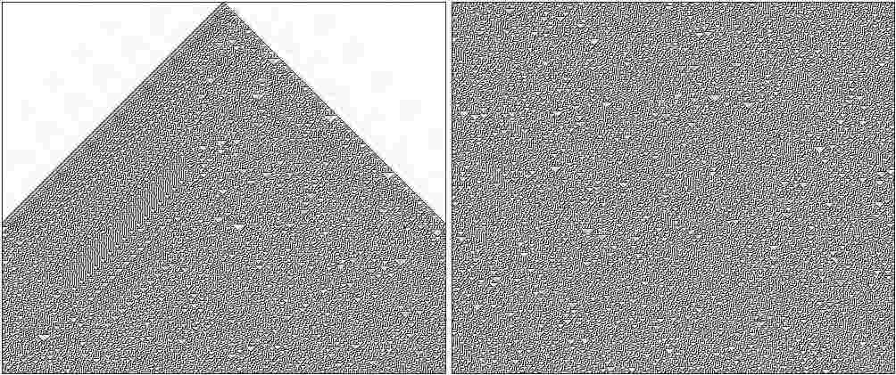
Figure 2: Typical behavior of Rule 30 where a single cell in state 1 leads to chaotic state (left). Second configuration (right) shows automaton behavior from a random initial condition with initial density of 50% for each state. Both automata evolve on a ring of 497 cells (with periodic boundary property) to 417 generations. White cells represent state 0 and dark cells the state 1.

Also the evolution rule presents the following feature: if an initial configuration is covered only of state one then the configuration always evolves into one but if this is empty or filled with state one then this always evolves to state zero. Fig. 2 shows such two cases of typical evolutions in Rule 30.

3.1 De Bruijn and subset diagrams in Rule 30

Given a finite sequence $w\in\Sigma^{m}$; such that $w=w_{1},\ldots,w_{m}$; let $\alpha(w)=w_{1}$, $\beta(w)=w_{2},\ldots,w_{m}$, and $\psi(w)=w_{1},\ldots,w_{m-1}$. With these elements, we can specify a labeled directed graph known as de Bruijn diagram $\mathcal{B}=\{N;E\}$ associated with the evolution rule of the CA. The nodes of $\mathcal{B}$ are defined by $N=\Sigma^{2r}$ and the set of directed edges $E\subseteq\Sigma^{2r}\times\Sigma^{2r}$ is defined as follows:

$$E=\{(v,w)\,\mid\,v,w\in N,\;\beta(v)=\psi(w)\}.$$ (5)

For every directed edge $(v,w)\in E$, let $\eta(v,w)=aw\in\Sigma^{2r+1}$ where $a=\alpha(v)$; that is, $\eta(v,w)$ is a neighborhood of the automaton. In this way, the edge $(v,w)$ is labeled by $\varphi\circ\eta(v,w)$; hence every labeled path in $\mathcal{B}$ represents the evolution of the corresponding sequence specified by its nodes. Since each $w\in N$ can be described by a number base $k$ of length $2r$, every node in $\mathcal{B}$ can be enumerated by a unique element in $\mathbb{Z}_{k^{2r}}$, which is useful to simplify the diagram. The de Bruijn diagram associated to Rule 30 is depicted in fig. 3; where black edges indicate the neighborhoods evolving into $0$ and the ones evolving into $1$ are shown by gray edges.

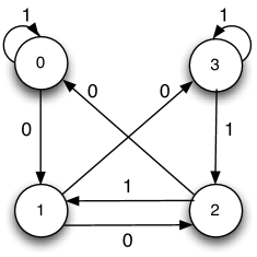
Figure 3: De Bruijn diagram for the elementary CA Rule 30.

Fig. 3 shows that there are four neighborhoods evolving into $0$ and four into $1$; so each state has the same probability to appear during the evolution of the automaton; indicating the possibility of the automaton is surjective, i.e. there are no Garden of Eden configurations. Classical analysis in graph theory has been applied over de Bruijn diagrams for studying topics such as reversibility [36]: cycles in the diagram indicate periodic elements in the evolution of the automaton if the label of the cycle corresponds to the sequence defined by its nodes, in periodic boundary conditions. The cycles in the de Bruijn diagram from fig. 3 are presented in fig. 4.

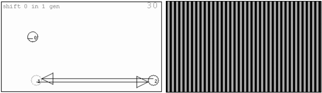
Figure 4: Cycles in the de Bruijn diagram and the corresponding periodic evolution for cycle $(1,2)$.

The largest cycle in fig. 4 indicates that the undefined repetition of sequence $w_{b}=10$ establishes a periodic structure without displacement in one generation during the evolution of Rule 30 we will than $w_{b}$ is the filter in Rule 30; in this case, the filter reported in the original Rule 30 and with memory too. Thus we can see how a de Bruijn diagram can recognize any periodic structures in CA [29, 24].

De Bruijn diagram is nondeterministic in the sense that a given node may have several output edges with the same label; a classical approach to analyse the diagram would be to construct the subset (or power) diagram in order to obtain a deterministic version for the de Bruijn diagram in the evolution rule [26, 38].

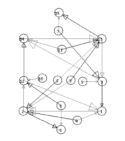
Figure 5: Subset diagram for Rule 30.

The subset diagram is defined as $\mathcal{S}=\{\mathcal{P},\mathcal{Q}\}$ where $\mathcal{P}=\{P\mid P\subseteq\Sigma\cup\emptyset\}$ is the set of nodes of $\mathcal{S}$ and the directed edges are defined by $\mathcal{Q}\subset\mathcal{P}\times\mathcal{P}$ where for $P_{1},P_{2}\in\mathcal{P}$ there is a directed edge $(P_{1},P_{2})$ labeled by $a\in S$ in $\mathcal{S}$ iff $P_{2}$ is the maximum subset such that for every $c\in P_{2}$ there exists $b\in P_{1}$ such that $\varphi(b,c)=a$.

The inclusion of the empty set assures that every edge has a well-defined ending node. For a CA with $k$ states, it is fulfilled that $|\mathcal{P}|=2^{k^{2r}}$ which implies an exponential growth in the number of nodes in $\mathcal{S}$ when more states are considered. Every $P\in\mathcal{P}$ can be identified by a binary number showing the states belonging to this subset; that is, taking the states as an ordered list, the ones in $P$ can be signed by a $1$ and the others by $0$; conforming a unique binary sequence identifying the subset. The decimal value of this binary number can be taken to get a shorter representation; where the empty set has a decimal number $0$ and the full subset $p=\Sigma$ has the number $2^{k^{2r}}-1$. The a subset diagram corresponding to Rule 30 is shown in fig. 5.

In fig. 5, the subset diagram has no path starting from the full subset (node $15$) going to the empty one (node $0$). This means that every sequence can be produced by the evolution of the automaton and there are no Garden-of-Eden sequences. Thus the automaton is surjective. The subset diagram can be also used as a deterministic automaton for calculating ancestors of any desired sequences [35] by recognizing the regular expressions which may be generated by the corresponding automaton. Some of these expressions would be able to represent interesting structures as gliders [30]; however more effort is needed in order to get a straightforward detection of such constructions in the diagram.

Finally, such diagrams helps to get periodic strings than eventually represent a general filter $w_{b}$ working at the original Rule 30 and Rule 30 with memory (next section). Also, we will take advantage of these results to find gliders from these strings.

4 Majority memory helps to discover complex dynamics in Rule 30

This section reports how the majority memory $\phi$ helps to discovers complex dynamics in elementary CA by experimentation, see an introduction to elementary CA with memory in [8, 9, 5].

In this way, fig. 6 displays different scenarios where the majority memory works on Rule 30 and therefore extracting complex dynamics on $\phi_{maj}$. We should read the evolutions from left to right and up to down. Also in this case all evolutions use the same random initial density and the filter $w_{b}$ was utilized in all evolutions (including the original Rule 30 evolution).

Thus the first evolution is the original function Rule 30, i.e, without majority memory in fig 6. From its original evolution we can see gaps that the filter can clean. Traditionally was difficult distinguish such filter in Rule 30 but when $\phi_{maj}$ was applied then its presence was more evident. A general technique to get filters was developed by Wuensche in [44].

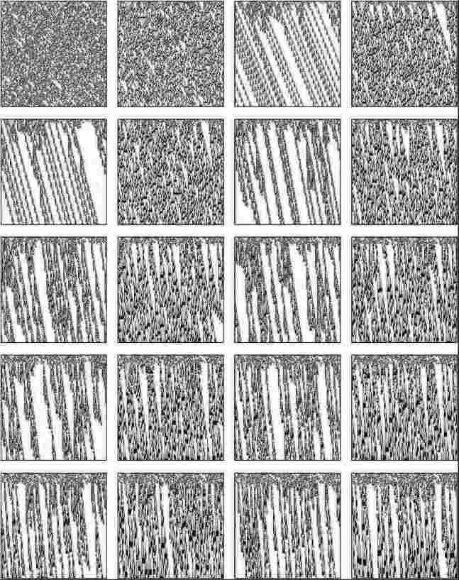
Figure 6: Complex dynamics emerging in Rule 30 with majority memory $\phi_{maj}$ from a range of values from $\tau=3$ to $\tau=21$ although the first evolution shows the original function. Evolutions were calculated on a ring of 104 cells in 104 generations with a random initial density of 50% where the initial condition is the same in all cases. Also the filter $w_{b}$ was applied to see clearly the structures.

Initially, even values of $\tau$ seems extract gliders more quickly and odd values fight to reach an order. Eventually the majority memory will converge to one stability in $\Phi$ while $\tau$ increases.

The first snapshot calculating $\phi_{maj}$ with $\tau=3$ was the second evolution in fig 6. Nevertheless, here is not very clear how the memory could induce another behavior because its global behavior is similar at the original but with small changes.

On the other hand, the third evolution with $\tau=4$ extracts periodic patterns emerging in Rule 30 with memory. The evolution maybe does not display impressive gliders but it already allows to pick up more diversity in mobile localizations on lattices of $100\times 100$ cells. Thus we have enumerated and ordered values of $\tau$ from fig. 6 based on their space-time dynamics they are responsible for.

1. Chaotic global behavior $\tau=0,3,5,7,9,11,13,15,17,19,21$.

2. Periodic patterns $\tau=4,6,8,10,12,14,16,18,19,20,21$.

3. Collision patterns $\tau=6,8,10,12$.

4.1 Morphological complexity in Rule 30 with memory

Looking a way to explore global complex dynamics in Rule 30 and itself with memory $\phi_{maj}$. In this section we will explore some techniques.

We evaluate morphological complexity of CA studied using morphological richness approach [4]. We calculate statistical morphological richness $\mu$ as follows. Given space-time configuration of a one-dimensional CA, for each site of the configuration we extract its $3\times 3$ cell space-time neighborhood state and build distribution of the space-time neighborhood states over extended period of the automaton’s development time.

Examples of morphological richness $\mu$ are shown in fig. 7. A control case, when next state of a cell is calculated at random the distribution (fig. 7a) of space-time neighborhood states is uniform. Two-dimensional random configurations are morphologically rich. Morphology of memoryless, classical, Rule 30 automaton is characterized by few peaks in local domains distributions, where several space-time templates dominate in the global space-time configuration (fig. 7b). The statistical morphological richness $\mu$ decreases.

Figure 7: Morphological richness. CA length 1500 cells, running time 5000 steps. (a) random update of cell states, (b) Rule 30 without memory, (c)–(f) with memory, (c) $\tau=3$, (d) $\tau=5$, (e) $\tau=10$, (f) $\tau=21$.

Incorporation of a memory in the cell-state transition rules leads to erosion of the distribution (fig. 7c) and thus slight increases in $\mu$. With increase of memory depth shape of the morphological distribution changes just slightly, up to minor variations in heights of major peaks (fig. 7d–f).

Number $\rho$ of $3\times 3$ blocks (of states 0 and 1) that never appear in space-time configurations of a cellular automaton can be used as a express estimate of the nominal morphological richness, the less $\rho$ the more rich is a nominally configuration.

The difference between statistical $\mu$ and nominal $\rho$ measures of morphological richness is that $\mu$ allows to pick up most common configurations of local domains, while $\rho$ just shows how many block of $3\times 3$ states appeared in the automaton evolution at least once.

For the case of random update of cell states, all blocks are present in the space-time configuration, $\rho=0$.

Memoryless automata governed by Rule 30 have $\rho=434$ (total number of possible blocks is 512). When memory is incorporated in the cell-state transition function, first richness decreases, e.g. for $\tau=1$, we have $\rho=448$. Then we observe consistent increase in complexity. Thus Rule 30 with small-depth memory ($\tau=2$) $\rho=140$, which drastically decrease to $\rho=68$ for $\tau=3$. The richness is stabilized, or rather oscillate around values $\rho=20-40$ with further increase of memory.

In summary, we found that majority memory increases nominal complexity of cellular automata but decreases statistical complexity.

4.2 Gliders in Rule 30 with memory $\tau=8$

Most frequently the complex dynamics related in elementary CA is related to gliders, glider guns, and non-trivial reactions between localizations, for example, Rule 110 or 54 [28, 23]. The relevance to look for such things is the study of universality [14, 42]. Another additional subject was its representation by regular expressions and other tools [29, 24].

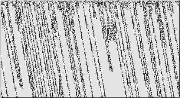
Figure 8: Gliders emerging in Rule 30 with $\phi_{maj}$ and $\tau=8$. This evolution shows how some kinds of gliders arise and still interact from random initial conditions. The evolution was calculated on a ring of 590 cells to 320 generations, and an initial density of 50%.

Among the sets of complex dynamics in Rule 30 determined by $\tau$ (showed in fig. 6), we have chosen the memory $\phi_{maj}$ with $\tau=8$. In this way, fig 8 illustrates an ample evolution space of its global dynamics.

Of course, these gliders maybe are not as impressive as others from well-known complex rules as Rule 110, Rule 54 or other one dimensional rules [12, 28, 23, 41, 43]. However it is interesting how $\phi_{maj}$ is able to open complex patterns from chaotic rules.

Nevertheless, even that Rule 30 does not offer an ample range of complex dynamics, it is useful to describe gliders and collisions. So, we shall illustrate how a chaotic CA can be discomposed as a complex system.

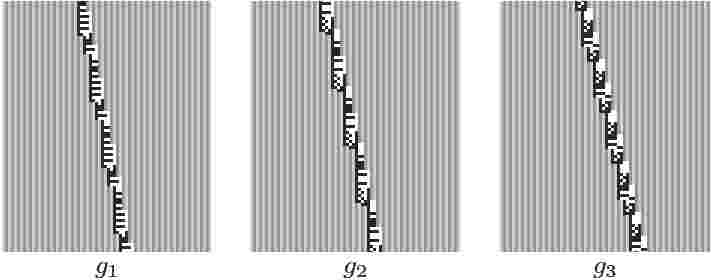
Figure 9: Set of gliders $G_{R30m}$ with memory $\phi_{maj}$ and $\tau=8$.

Thus we classify the family of gliders and enumerate some properties. Then fig. 9 displays the family of gliders $G_{R30m}=\{g_{1},g_{2},g_{3}\}$. Although as was hoped, an immediate consequence was that gliders in CA with memory have longer periods.

structure	$v_{g}$	lineal volume
$w_{b}$	$0/c$ = 0	2
$g_{1}$	$2/11\approx 0.1818$	5
$g_{2}$	$4/19\approx 0.2105$	7
$g_{3}$	$4/17\approx 0.2352$	6

Table 1: Properties of gliders $G_{R30m}$ with memory $\phi_{maj}$ and $\tau=8$.

Tab. 1 summarizes the basic properties of each glider. Particularity all gliders in this domain have a constant displacement of four cells to the right and none glider with speed zero was founded, and yet it was more complicated to find a glider gun in this domain. Nevertheless, some interesting reactions were originated from $G_{R30m}$.

Structure $w_{b}$ does not have a displacement and also it is neither a glider. This pattern is the periodic background in Rule 30 and still represent the filter in Rule 30. It was really hard to detect the existence of a periodic background evolving the original rule; but when $\phi_{maj}$ was applied, a periodic pattern began to emerge inherited from $\varphi_{R30}$. Finally this filter was confirmed with its respective de Bruijn and cycle diagrams (see section 3.1).

4.3 Reactions between gliders from $G_{R30m}$

Let us demonstrate simple examples of collisions between gliders. Codes for all gliders, necessary to generate the whole set of binary collisions, are presented in appendixes A and B.

Fig. 10 shows how a stream of $g_{1}$ gliders is deleted from a reaction cycle:

$$g_{3}+g_{1}\rightarrow g_{2}\mbox{ and }g_{2}+g_{1}\rightarrow g_{3}.$$

Figure 10: Deleting streams of $g_{1}$ gliders initialized with a single $g_{3}$ glider.

To obtain such cycle by glider reaction we can code an unlimited initial condition as $...g_{3}...g_{1}....g_{1}....g_{1}....$, that can be reduced as $...g_{3}...g_{1}(....g_{1})^{*}$ (where a dot represent a copy of $w_{b}$). Finally the evolution produces the cycle above, which is produced with nine periods of $g_{3}$ and eight periods of $g_{2}$. Thus each column presents 1135, 2270 and 3405 generations respectively.. However in this case the codification of gliders is affected because could not natural as was done in other cases [28, 29, 24].

Since the better way to preserve $\varphi_{R30}$ and $\phi_{maj}$ to code gliders as “natural,” we will consider the codification from its original initial condition (see appendix B where some strings are defined to get gliders with memory from its original function).

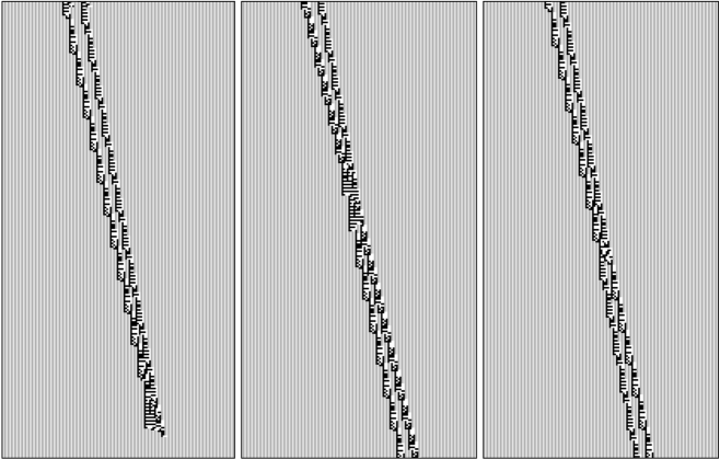
Figure 11: Some simple reactions display how to delete (left), read (centre) and preserve (rigth) information with gliders in Rule 30 with memory.

Some simple but interesting reactions from $G_{R30m}$ are illustrated in the fig. 11. First reaction is annihilation of gliders $g_{2}$ and $g_{1}$. Second reaction is a transformation $g_{3}$ glider transforms $g_{1}$ glider to $g_{2}$. Third reaction is a soliton-like collision between gliders $g_{2}$ and $g_{1}$. The soliton reaction between gliders is particularly promising because it can be used to implement computation, e.g. as it has been done in carry-ripple adder embedded by phase coding solitons in parity CA [32, 19].

4.4 Quasi-chemistry of gliders

Assuming gliders $g_{1}$, $g_{2}$ and $g_{3}$ are chemical species $a$, $b$ and $c$ in a well-stirred chemical reactor we can derive the following set of quasi-chemical reactions from the interactions between the gliders above:

$$\begin{array}[]{l}a+b\stackrel{{\scriptstyle 0.6}}{{\rightarrow}}\epsilon\\ a+b\stackrel{{\scriptstyle 0.2}}{{\rightarrow}}2a\\ a+b\stackrel{{\scriptstyle 0.2}}{{\rightarrow}}c\\ a+c\stackrel{{\scriptstyle 0.44}}{{\rightarrow}}b\\ a+c\stackrel{{\scriptstyle 0.12}}{{\rightarrow}}b+c\\ a+c\stackrel{{\scriptstyle 0.22}}{{\rightarrow}}3a\\ a+c\stackrel{{\scriptstyle 0.22}}{{\rightarrow}}a\\ b+c\stackrel{{\scriptstyle 0.5}}{{\rightarrow}}b\\ b+c\stackrel{{\scriptstyle 0.5}}{{\rightarrow}}2a+b\end{array}$$ (6)

where reaction rates are evaluated from the frequencies of the interactions.

Figure 12: Dynamics of concentrations of species $a$ (circle), $b$ (diamond) and $c$ (square) governed by reaction eqs. 6. (a) Initial concentrations of all species are 0.001 mole/l. (b) Initial concentrations of species $b$ and $c$ are 0.001 mole/l, species $a$ is nil. Horizontal axes is a time in $10^{-3}$ sec.

We evaluated global dynamics of the quasi-chemical system (6) with constant volume (which reflects finite size of the automaton lattice), constant temperature, and variable pressure using Chemical Kinetics Simulator. Fig. 12 shows temporal dynamics of species concentrations in the system with $10^{7}$ molecules.

In the initial conditions when all three species are present in equal concentrations (fig. 12a) we observe exponential decay of species $b$ and $c$ and stabilization of concentration of species $a$. When only species $b$ and $c$ are present in a well-stirred reaction initially, they produce species $c$ in their reactions. This leads to outburst in species $a$ concentration (fig. 12b) on the background of exponential decline of species $c$ and $b$, until species $b$ and $c$ disappear and concentration of species $a$ becomes constant.

4.5 Glider machines

Experimentally found interactions between gliders can be simplified as follows, depending on distance $\sigma$ between interacting gliders:

$$\begin{array}[]{llll}\begin{array}[]{l}\sigma=3\\ b+a\rightarrow\{a,b\}\\ c+a\rightarrow b\\ c+b\rightarrow b\end{array}&\begin{array}[]{l}\sigma=4\\ b+a\rightarrow\{\emptyset\}\\ c+a\rightarrow b\\ c+b\rightarrow b\end{array}\begin{array}[]{l}\sigma=5\\ b+a\rightarrow\{\emptyset\}\\ c+a\rightarrow\{b,c\}\\ c+b\rightarrow\{a,b\}\end{array}\begin{array}[]{l}\sigma=6\\ b+a\rightarrow a\\ c+a\rightarrow\{b,c\}\\ c+b\rightarrow\{a,b\}\end{array}\end{array}$$

Taking into account gliders’ velocities (tab.1), we can construct the following finite state indeterministic machine with an internal state $h$ and input state $p$, $h,p\in\{a,b,c,\emptyset\}$. The machine can be characterised by an input-output transition matrix $M=(m_{ij})_{i,j\in\{a,b,c,\emptyset\}}$, where for $j=h^{t}$, $i=p^{t}$, $m_{ij}=h^{t+1}$. The matrix has the following form:

$$M=\begin{array}[]{l|llll}h^{t+1}&a&b&c&\emptyset\\ \hline\cr a&a&\{a,\emptyset\}&b&a\\ b&b&b&\{a,b\}&b\\ c&c&c&c&c\\ \emptyset&\emptyset&\emptyset&\emptyset&\emptyset\end{array}$$

Starting at a randomly chosen initial state and subjected to random uniformly distributed input strings the machine will end in the state $c$ with probability $\frac{1}{4}$ and in the state set with probability $\frac{3}{3}{4}$. The machine starting in the initial $h$ generates the string $l(h)$ as follows: $l(\emptyset)=\emptyset^{*}$, $l(a)=(ab^{*}a^{*})^{*}\emptyset^{*}$,$l(b)=(b^{*}a^{*})^{*}\emptyset^{*}$, $l(c)=c^{*}$.

5 Discussion

We enriched elementary CA rule 30 with majority memory and demonstrated that by applying certain filtering procedures we can extract rich dynamics of travelling localizations, gliders, and infer sophisticated system of quasi-chemical reactions between the gliders. We shown that the majority memory increases nominal complexity but decreases statistical complexity of patterns generated by the CA. By applying methods of de Brujin diagrams and graph theory we proved that surjectivity of Rule 30 CA with memory and provide blue prints for future detailed analysis of glider dynamics.

Figure 13: New family of elementary CA composed.

Recalling previous results on classification of one-dimensional CA [40, 43, 44] we envisage that introduction of majority memory $\phi_{maj}$ into elementary CA will open a new field of research in selection of non-trivial rules of cell-state transitions and precise mechanics of relationships between chaotic and complex systems.

This is because Rule 30 was grouped into a cluster of rules with similar behaviour, that can be transformed one to another using combinations of reflexion, negation and complement (done by Wuensche in [40]). This way fig. 13 shows a diagram that explains how the original cluster for Rule 30 is presented in [40]. Obviously the cluster can be arbitrarily enriched using not only $\phi_{maj}$ but any types of memory and $\tau$. Thus the dynamical complexity of automata with $\phi_{maj}$ is the same as for the set of function $\{\varphi_{R30},\varphi_{R86},\varphi_{R135},\varphi_{R149}\}$, particularly because the local functions $\varphi_{R86}$ and $\varphi_{R149}$ are responsible for leftward motion of gliders.

Therefore, memory in elementary CA and others families of CA offer a new approach to discover complex dynamics based on gliders and non-trivial interactions between gliders. This can be substantiated by a number of different techniques, e.g. number-conservation [11, 18], exhaustive search [17], tiling [29, 22], de Bruijn diagrams [24], $Z$-parameter [44], genetic algorithms [16], mean field theory [25] or from a differential equations point view [13].

Appendix A. Binary reactions and beyond

We represent binary collisions in Rule 30, $\phi_{maj}$ and $\tau=8$ in the form $g_{j}\xrightarrow{space}g_{i}$, where $j>i$, $g\in G_{R30}$ and space is the interval between gliders given by the number of strings $w_{b}$. Collisions producing $\epsilon$ mean annihilation of gliders. Reactions are developed using increasing the distance between gliders before collision.

Collisions of type $g_{2}\rightarrow g_{1}$

1. $g_{2}\xrightarrow{3}g_{1}=g_{1}+g_{2}$ (soliton)

2. $g_{2}\xrightarrow{4}g_{1}=\epsilon$

3. $g_{2}\xrightarrow{5}g_{1}=\epsilon$

4. $g_{2}\xrightarrow{6}g_{1}=2g_{1}$

5. $g_{2}\xrightarrow{7}g_{1}=\epsilon$

6. $g_{2}\xrightarrow{8}g_{1}=g_{3}$

Collisions of type $g_{3}\rightarrow g_{1}$

1. $g_{3}\xrightarrow{3}g_{1}=g_{2}$

2. $g_{3}\xrightarrow{4}g_{1}=g_{2}$

3. $g_{3}\xrightarrow{5}g_{1}=g_{2}+g_{3}$

4. $g_{3}\xrightarrow{6}g_{1}=g_{1}^{3}$

5. $g_{3}\xrightarrow{7}g_{1}=g_{1}+g_{1}^{2}$

6. $g_{3}\xrightarrow{8}g_{1}=g_{2}$

7. $g_{3}\xrightarrow{9}g_{1}=g_{1}$

8. $g_{3}\xrightarrow{10}g_{1}=g_{2}$

9. $g_{3}\xrightarrow{11}g_{1}=g_{1}$

Collisions of type $g_{3}\rightarrow g_{2}$

1. $g_{3}\xrightarrow{3}g_{2}=g_{2}$

2. $g_{3}\xrightarrow{4}g_{2}=g_{2}$

3. $g_{3}\xrightarrow{5}g_{2}=2g_{1}+g_{2}$

4. $g_{3}\xrightarrow{6}g_{2}=2g_{1}+g_{2}$

Some other reactions with packages of gliders

1. $g_{2}\xrightarrow{5}2g_{1}=g_{1}$

2. $g_{2}\xrightarrow{8}2g_{1}=3g_{1}$

3. $g_{2}\xrightarrow{10}2g_{1}=g_{2}$ (sequence $g_{2}$, $g_{3}$, $g_{2}$)

4. $2g_{2}\xrightarrow{6}g_{1}=3g_{1}$

5. $2g_{2}\xrightarrow{7}g_{1}=g_{2}$

6. $2g_{2}\xrightarrow{8}g_{1}=g_{1}+g_{3}$

7. $g_{3}\xrightarrow{5}2g_{1}=\epsilon$

8. $g_{3}\xrightarrow{6}2g_{1}=g_{3}$

9. $g_{3}\xrightarrow{7}2g_{1}=g_{1}+g_{2}$

10. $g_{3}\xrightarrow{8}2g_{1}=g_{1}^{3}+g_{1}$

11. $g_{3}\xrightarrow{9}2g_{1}=g_{1}^{4}$

12. $g_{3}\xrightarrow{10}2g_{1}=2g_{1}$

13. $2g_{3}\xrightarrow{5}g_{2}=g_{2}$ (wall)

Appendix B. Coding gliders $G_{R30m}$

We can enumerate strings conforming gliders in Rule 30 with $\phi_{maj}$ and $\tau=8$, in given initial conditions and using “phases” (we omit strings that do not produce gliders).

Note that such strings evolve initially with $\varphi_{R30}$ and a value of $\tau$ given, then $\phi_{maj}$ will open these strings when memory works. Thus we can code initial conditions with gliders in CA with memory, that also was implemented in OSXLCAU21 system to get our simulations.

$g_{1}$ glider	$g_{2}$ glider	$g_{3}$ glider
1 – $g_{1}$	100 – $g_{2}$	110110 – $2g_{1}$ join
111 – $g_{1}$	111 – $g_{1}$	101110 – $g_{3}$
10000 – $g_{1}$	10000 – $g_{1}$	111100 – $2g_{1}$
11110 – $g_{1}$	11110 – $g_{1}$	100011 – $2g_{1}$ join
100 – $g_{2}$	1100110 – $g_{2}+g_{3}$	1011 – $g_{3}$
11110 – $g_{1}$	1010110 – $g_{1}$
10000 – $g_{1}$	1101100 – $g_{2}$
11001 – $g_{2}+g_{3}$

Table 2: Strings evolving in gliders of $G_{R30m}$.

Tab. 2 enumerates strings for each glider represented as a tiling so we know their “phases” [28, 29]. Although in this case, it was difficult to classify such strings as regular expressions because not all strings from the tiling representation evolve into gliders.

References

- [1] Amoroso, S. & Cooper, G. (1970) The Garden-of-Eden theorem for finite configurations, Proceedings of the American Mathematical Society.
- [2] Adamatzky, A. (1994) Identification of Cellular Automata, Taylor and Francis, London.
- [3] Adamatzky, A. (ed.) (2003) Collision-Based Computing, Springer.
- [4] Adamatzky, A. & Holland, O. (1998) Phenomenology of excitation in 2-D cellular automata and swarm systems, Chaos, Solitons & Fractals 9 1233–1265.
- [5] Alonso-Sanz, R. (2006) Elementary rules with elementary memory rules: the case of linear rules, Journal of Cellular Automata 1 71–87.
- [6] Alonso-Sanz, R. (2008) Cellular Automata with Memory, Old City Publishing, Inc.
- [7] Alonso-Sanz, R. (2009) Cellular automata with memory. In Meyers, R. (Ed.) Encyclopedia of Complexity and Systems Science, Springer NY, (in press).
- [8] Alonso-Sanz, R. & Martin, M. (2003) Elementary CA with memory, Complex Systems 14 99–126.
- [9] Alonso-Sanz, R. & Martin, M. (2005) One-dimensional Cellular Automata with Memory in cells of the most recent value, Complex Systems 15 (3) 203–236.
- [10] Bar-Yam, Y. (1997) Dynamics of Complex Systems, Perseus Books.
- [11] Boccara, N. & Fukś, H. (2002) Number-Conserving Cellular Automaton Rules, Fundamenta Informaticae 52 1–13.
- [12] Boccara, N., Nasser, J., & Roger, M. (1991) Particle like structures and their interactions in spatio-temporal patterns generated by one-dimensional deterministic cellular automaton rules, Physical Review A 44 (2) 866–875.
- [13] Chua, L.O. (2007) A Nonlinear Dynamics Perspective of Wolfram’s New Kind of Science, World Scientific Publishing Company.
- [14] Cook, M. (2004) Universality in Elementary Cellular Automata, Complex Systems 15 (1) 1–40.
- [15] Culik II, K. & Yu, S. (1988) Undecidability of CA Classification Schemes, Complex Systems 2 177–190.
- [16] Das, R., Mitchell, M., & Crutchfield, J.P. (1994) A genetic algorithm discovers particle-based computation in cellular automata, Lecture Notes in Computer Science 866 344–353.
- [17] Eppstein, D. (2002) Searching for spaceships, MSRI Publications 42 433–452.
- [18] Imai, K., Ikazaki, A., Iwamoto, C., & Morita, K. (2004) A logically universal number-conserving cellular automaton with a unary table-lookup function, IEICE Trans. on Information and Systems E87-D 694–699.
- [19] Jakubowski, M.H., Steiglitz, K., & Squier, R. (2001) Computing with Solitons: A Review and Prospectus, Multiple-Valued Logic 6 (5-6) (also republished in [3]).
- [20] Kauffman, S.A. (1993) The Origins of Order: Self-Organization and Selection in Evolution, Oxford University Press, New York.
- [21] Steiglitz, K., Kamal, I., & Watson, A. (1988) Embedding Computation in One-Dimensional Automata by Phase Coding Solitons, IEEE Transactions on Computers 37 (2) 138–145.
- [22] Margenstern, M. (2007) Cellular Automata in Hyperbolic Spaces, Old City Publishing, Inc.
- [23] Martínez, G.J., Adamatzky, A., & McIntosh, H.V. (2006) Phenomenology of glider collisions in cellular automaton Rule 54 and associated logical gates, Chaos, Solitons and Fractals 28 100–111.
- [24] Martínez, G.J., Adamatzky, A., & McIntosh, H.V. (2008) On the representation of gliders in Rule 54 by de Bruijn and cycle diagrams, Lecture Notes in Computer Science 5191 83–91.
- [25] McIntosh, H.V. (1990) Wolfram’s Class IV and a Good Life, Physica D 45 105–121.
- [26] McIntosh, H.V. One Dimensional Cellular Automata, by publish.
- [27] Minsky, M. (1967) Computation: Finite and Infinite Machines, Prentice Hall.
- [28] Martínez, G.J., McIntosh, H.V., & Seck-Tuoh-Mora, J.C. (2006) Gliders in Rule 110, Int. J. of Unconventional Computing 2 (1) 1–49.
- [29] Martínez, G.J., McIntosh, H.V., Seck-Tuoh-Mora, J.C., & Chapa-Vergara, S.V. (2008) Determining a regular language by glider-based structures called phases fi_1 in Rule 110, Journal of Cellular Automata 3 (3) 231–270.
- [30] Martínez, G.J., McIntosh, H.V., Seck-Tuoh-Mora, J.C., & Chapa-Vergara, S.V. (2008) A note about the regular language of Rule 110 and its general machine: the scalar subset diagram, Proceedings 3rd. International Workshop on Natural Computing, IWNC 2008, Yokohama, Japan, 39–49.
- [31] Mitchell, M. & Newman, M. (2002) Complex Systems Theory and Evolution, In Encyclopedia of Evolution (Pagel, M., ed.), Oxford University Press.
- [32] Park, J.K., Steiglitz, K., & Thurston, W.P. (1986) Soliton-like behavior in automata, Physica D 19 423–432.
- [33] Robinson, C. (1994) Dynamical Systems: stability, symbolic dynamics and chaos, CRC Press.
- [34] Rowland, E.S. (2006) Local Nested Structure in Rule 30, Complex Systems 16 (3) 239–258.
- [35] Seck-Tuoh-Mora, J.C., Martínez, G.J., & McIntosh, H.V. (2004) Calculating ancestors in one-dimensional cellular automata, Int. J. of Modern Physics C 15 (8) 1151–1169.
- [36] Seck-Tuoh-Mora, J.C., Chapa-Vergara, S.V., Martínez, G.J., & McIntosh, H.V. (2005) Procedures for calculating reversible one-dimensional cellular automata, Physica D 202 134–141.
- [37] Sipper, M. (1997) Evolution of Parallel Cellular Machines: The Cellular Programming Approach, Springer-Verlag, Heidelberg.
- [38] Voorhees, B.H. (1996) Computational analysis of one-dimensional cellular automata, World Scientific Series on Nonlinear Science, Series A, Vol. 15.
- [39] von Neumann, J. (1966) Theory of Self-reproducing Automata (edited and completed by A. W. Burks), University of Illinois Press, Urbana and London.
- [40] Wuensche, A. & Lesser, M. (1992) The Global Dynamics of Cellular Automata, Santa Fe Institute Studies in the Sciences of Complexity, Addison-Wesley Publishing Company.
- [41] Wolfram, S. (1994) Cellular Automata and Complexity, Addison-Wesley Publishing Company.
- [42] Wolfram, S. (2002) A New Kind of Science, Wolfram Media, Inc., Champaign, Illinois.
- [43] Wuensche, A. (1994) Complexity in one-d cellular automata, Santa Fe Institute working paper 94-04-025.
- [44] Wuensche, A. (1999) Classifying Cellular Automata Automatically, Complexity 4 (3) 47–66.