Return probabilities and hitting times of random walks on sparse Erdös-Rényi graphs

Abstract

We consider random walks on random graphs, focusing on return probabilities and hitting times for sparse Erdös-Rényi graphs. Using the tree approach which is expected to be exact in the large graph limit, we show how to solve for the distribution of these quantities and we find that these distributions exhibit a form of self-similarity.

I Introduction

Random walks are some of the simplest stochastic processes Hughes (1996); Bouchaud and Georges (1990) and yet they arise in many scientific fields such as pure mathematics, statistical physics or even biology Montroll and Shuler (1979); Newman (2005); Noh and Rieger (2004); Benichou et al. (2005). A fundamental quantity for computing properties of random walks is the first passage time Feller (1950); Redner (2001). Consider a random walk on a graph $G$, starting at node $s$; given another arbitrary node $t$ (the target), the hitting time $H(s,t)$ is just the mean of the first passage time to go from $s$ to $t$. There is a well known relation between the value of $H(s,t)$ averaged over all nodes $t$ of the graph and the spectrum of its adjacency matrix, as derived in Lovász (1993).

In this work we focus on random graphs Bollobás (2001); Lovász (1993). For dense Erdös-Rényi graphs Erdös and Rényi (1959), the spectrum of the diffusion operator converges to that of a Gaussian random matrix and one can show Chung et al. (2003); Sood et al. (2005) that if $N$ is the number of nodes of $G$, the hitting time is $N+o(N)$. As far as we know, there is no analogous result for sparse graphs: only a mean-field approximation has been derived Baronchelli and Loreto (2006) which neglects certain fluctuations. This situation is surprising because the problem has been open for many years, but the lack of progress underlies the difficulty of deriving analytically the spectrum of the adjacency matrix on sparse random graphs Biroli and Monasson (1999); Semerjian and Cugliandolo (2002). Nevertheless, we here bypass this difficulty by exploiting the local structure of sparse random graphs that is tree-like with probability $1$ at large $N$. If, as in a number of other problems Aldous (2001); Mézard et al. (2002), only the graph’s local structure matters at large $N$, then the problem maps in the $N\to\infty$ limit to diffusion processes on random trees. This tree approach, which will be validated in Sect. VII, then provides an analytical calculation for the hitting times and for a closely related quantity, the probability that the walker returns to its starting node in a finite time.

In what follows, we first specify the stochastic dynamics of the random walk and the kinds of random graphs we use. After we compute the hitting times and probabilities of return on random $d$-regular graphs Wormald (1999). That calculation is then generalized to sparse Erdös-Rényi graphs, displaying quite subtle distributions.

II The model

We consider a random walker on a graph $G$. At each time step $n$, the walker hops to one of the neighboring nodes, all such nodes being equi-probable. It is convenient to introduce the adjacency matrix $A$ of $G$: $A_{ij}=1$ if nodes $i$ and $j$ are connected by an edge and $A_{ij}=0$ otherwise. Defining at each time step $n$ the probability $\mathbf{v}_{i}^{(n)}$ of having the walker be at node $i$, the vector of probabilities obeys the master equation

$$\mathbf{v}_{i}^{(n+1)}=\sum_{<ji>}\frac{1}{d_{j}}\mathbf{v}_{j}^{(n)}=\left(AD^{-1}\mathbf{v}^{(n)}\right)_{i}$$ (1)

where the sum is taken over all nodes $j$ that are adjacent to the node $i$. The matrix $D$ is diagonal; its $i$-th diagonal element $D_{ii}$ is equal to the degree $d_{i}$ of the $i$-th node.

To investigate the hitting time of the walker to go from node $s$ to $t$, it is enough to initialize the vector $\mathbf{v}^{(0)}$ to be zero on all nodes except at $s$ where it is 1, and to impose absorbing conditions at the target node $t$, i.e., $\mathbf{v}_{t}^{(n)}=0$ at all $n$. Then the probability of having a first passage time equal to $n$ is given by the flux into node $t$ at that time step Feller (1950). A modified treatment of the walker allows one to also obtain the probability of return to the starting node.

Our mathematical solution concerns Erdös-Rényi graphs in the ensemble $G(N,p)$, where $N$ is the total number of nodes and each pair of nodes has probability $p$ to be connected by an edge. For sparse graphs, $p=c/N$ where $c=\langle d\rangle$ is the mean degree of nodes. We shall also consider fixed degree random graphs, also called random $d$-regular graphs, where each node has the same degree $d$ and connections are otherwise random Wormald (1999).

III Hitting times on random $d$-regular graphs

Let us first compute the hitting time on random regular graphs, exploiting their local tree-like nature. Clearly, loops can arise in random $d$-regular graphs Wormald (1999) but their typical length is $O(\ln(N))$. Thus it is expected that most properties can be obtained by studying what happens locally, as long as boundary conditions at “infinity” are properly handled. Such an approach has been used in many contexts with a high level of success Aldous (2001); Mézard et al. (2002).

For a given random regular graph, of fixed degree $d$, we consider a node $t$ and ask what is the mean of $H(s,t)$ when averaged over all possible departing nodes $s$. We need to solve a diffusion problem where at time $n=0$ a walker is equi-distributed amongst the $N-1$ nodes $s$ ($s\neq t$) and if the walker hits node $t$ it gets absorbed. If one denotes by $F_{t}^{(n)}$ the probability flux into node $t$ at step $n$, then the hitting time averaged over all $s$ is given by the first moment of $n$ distributed according to $F_{t}^{(n)}$.

In the neighborhood of $t$, the graph is a Cayley tree with probability one at large number of nodes $N$ and thus does not depend on the node which we choose as absorbing in the large $N$ limit. Given the diffusion-absorption process, the vector of probabilities quickly converges to the dominant eigenvector of the master equation (that with the largest eigenvalue, decaying the slowest). In the limit of large $N$, the decay rate goes to zero and all the transient behavior (associated with the other eigenvectors) becomes irrelevant. When $N\to\infty$, it is then enough to determine the dominant eigenvector, imposing zero boundary condition at the root node $t$ and $1/(N-1)$ boundary conditions for the far away nodes.

As $N\to\infty$, the recurrence equation that is satisfied by the eigenvector’s elements leads to $dA_{k+1}=A_{k+2}+(d-1)A_{k}$ where $A_{k}$ is the sum of the probabilities on the nodes that are at distance $k$ from the root node. Solving this, subject to the normalization and boundary conditions, leads to the value of $A_{1}$ and thus the flux flowing into the absorbing node using the eigenvector: $F_{t}=A_{1}/d$.

Note that since at large $N$ only the leading eigenvector matters, the first passage time is exponentially distributed with a mean given by the inverse of this flux. This then gives for random $d$-regular graphs a hitting time behaving at large $N$ as

$$\frac{H}{N}=\frac{d-1}{d-2}+o(1)\ .$$ (2)

Finally, it is worth noting that for random $d$-regular graphs, with probability 1 in the large $N$ limit, the ratio $H(s,t)/N$ does not depend on the starting node $s$. Also, because of the regularity of the graph, this quantity does not depend on $t$ either.

IV Probability of return on random $d$-regular graphs

On any finite graph, a walker leaving node $t$ will return with probability one. Nevertheless, if one considers the distribution of return times for increasing values of $N$, one will find that there is a $N\to\infty$ limiting point-wise distribution but which does not integrate to 1. Indeed, in that limit, the return times will be finite with probability $\hat{r}$ and will diverge linearly in $N$ with probability $1-\hat{r}$. If $\hat{r}\neq 1$, the walk is said to be transient. On the infinite Cayley tree, $\hat{r}$ can be computed simply by using the homogeneity of the graph as follows.

Take $t$ to be the root of an infinite Cayley tree. The walker must make a first step; let it be to one of its neighbors $j$. Define $r$ as the probability for the walk to return to $t$ given that it has stepped to $j$. Using the equivalence of all nodes, one can write a series for $r$:

$$r=\frac{1}{d}+\frac{(d-1)r}{d}\frac{1}{d}+\frac{((d-1)r)^{2}}{d^{2}}\frac{1}{d}+\ldots$$ (3)

where $d\geq 2$ is the degree of the Cayley tree. In this series, the term of $O(r^{p})$ corresponds to the probability that the walk returns $p$ times to node $j$ before going back to the root $t$. Summing this geometric series gives two possible values: $r=1$ and $r=1/(d-1)$. Furthermore, it is easy to see that $\hat{r}=r$. If $d=2$, we have a one dimensional walker and $\hat{r}=1$. For $d\geq 3$, the walk is transient and $\hat{r}=1/(d-1)$.

V Probability of return on Erdös-Rényi graphs

Here we extend the previous calculation of return probabilities to the case of Erdös-Rényi graphs. Just as for the random $d$-regular graphs, we exploit the fact that with probability $1$ in the large $N$ limit the neighborhood of a node belonging to a sparse Erdös-Rényi graph is locally tree-like. We denote by $c=\langle d\rangle$ the mean degree of these graphs; the probability to have a node of degree $d$ is $P(d)=e^{-c}c^{d}/d!$, i.e., is given by the Poisson distribution.

To find the probability to return in a finite number of steps (formally at infinite $N$) for a walker starting on the root node $t$, we reconsider the series of Eq. (3). Suppose that at the first step the walker moves to the neighbor $j$ of the root node, and that $d_{j}$ is the connectivity of that node. If the walker is to return to $t$, it can do so immediately, or it can perform $p$ loops from $j$ (avoiding $t$), stepping back to $t$ only after its $(p+1)$th visit to node $j$. By a loop from $j$, we mean a step to one of the $d_{j}-1$ neighbors of $j$ other than $t$, then a finite number of steps that do not visit $j$, and then finally a return to $j$. The point is that in our system the walker cannot come back to $t$ other than through the edge connecting $j$ to $t$: any other route requires going to “infinity” and thus an infinite number of steps. (Since we are dealing with the return probability on an infinite graph, the walks returning to $t$ must have a finite number of steps.)

For the edges connecting node $j$ to a node other than $t$, let the return probabilities be $r_{j}(1)$, $r_{j}(2)$, …$r_{j}(d_{j}-1)$. Given these $r_{j}$s, the probability $r$ to return to the root node if the walk’s first step is to node $j$ is

$$r=\frac{1}{d_{j}-\sum_{m=1}^{d_{j}-1}r_{j}(m)}\,.$$ (4)

However, the $r_{j}(m)$ are i.i.d. random variables belonging to a distribution $\rho(r)$. In the Erdös-Rényi ensemble, $t$ connects to a random node ($j$ here) which itself connects to other random nodes. The distribution of $r$ is thus the same as that of the $r_{j}$s, and Eq. (4) determines implicitly a self-consistent functional equation for $\rho(r)$. This can be written formally as:

$$\rho(r)=P(0)\delta(1-r) + \sum_{z=1}^{\infty}P(z)\int dr_{1}\ldots\int dr_{z}$$ (5)

$$\rho(r_{1})\ldots\rho(r_{z}) \times \delta\left(\frac{1}{1+\sum_{i=1}^{z}(1-r_{i})}-r\right)$$

where $P(z)$ is the Poisson distribution (of $z=d_{j}-1$), and $\delta(x)$ is the Dirac delta function. Note that since we are dealing with an Erdös-Rényi graph, the probability that the node $j$ (which by construction is connected to the absorbing node $t$) has degree $z+1$ is given by $P(z)$. This is due to the fact that for Erdös-Rényi graphs, the edges are independent.

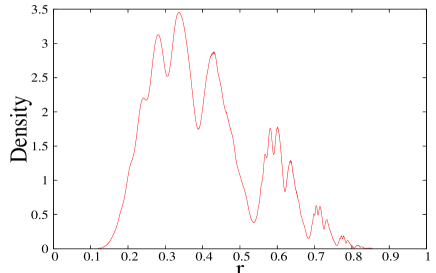
We have solved for $\rho$ by numerical iteration, demanding a stable distribution. Because $\rho$ has both a continuous part for $0\leq r<1$ and a delta function part at $r=1$, it was necessary to treat these two parts separately, and the the convergence in the number of iterations is quite fast. To illustrate our results, we display in Fig. 1 the probability density $\rho(r)$ when the mean degree is $3$. (Numerically, we must introduce a coordination cut-off and binning to compute $\rho(r)$; we find that taking a cut-off value of a few times the graph’s mean coordination leads to negligible errors, while beyond 2500 bins no visible dependence on bin size can be seen. For all the figures presented here, we used $10000$ bins.) It also exhibits a form of self-similarity: the motif for $0<r<0.5$ is repeated at larger values of $r$ but each time with a smaller amplitude and some distortion. Also, note that the distribution is relatively smooth; its continuity can be justified as follows. Consider the ensemble of graphs for which the return probability $r$ is in the interval $[r,r+dr]$. If we increase slightly the degree of a node far away from the absorbing node for all of these graphs, the return probability $r$ will decrease slightly. If this modified node is sufficiently far, the change in $r$ can be made arbitrarily small. Because of this, the distribution of $r$ can have no discontinuities.

Figure 1: (Color online) The probability density of the return probability $r$ after stepping from a given node to one of its neighbors on an infinite Erdös-Rényi graph with mean degree 3. For ease of presentation, the delta function contribution at $r=1$ has been removed and the rest has been rescaled to have a total probability of 1. Note the qualitative self-similarity.

As a last point, the intensity $\Delta$ of the Dirac part of $\rho$ gives the probability for the first step of the walk to connect to a finite part of the graph. It is thus simply given Bollobás (2001) by the solution to the equation $\Delta=\sum_{k=0}^{\infty}P(k)\Delta^{k}$, obtained by forcing the node $j$ to have all its neighbors in a finite part of the graph also. In such a situation, one has $r=1$.

VI Hitting times on Erdös-Rényi graphs

To compute the hitting time $H(s,t)$, we take $s$ and $t$ to be on the same connected component whose size we denote by $N_{\infty}$. For Erdös-Rényi graphs, we work beyond the percolation threshold, $c>1$, on the “infinite” component, so $N_{\infty}\simeq(1-\Delta)N$. With probability $1$, the hitting time $H(s,t)$ scales with $N$, has negligible fluctuations with $s$, and depends only the neighborhood properties of $t$. We thus focus on $H_{t}$, the mean of $H(s,t)$ when averaging over all nodes $s$ distinct from $t$. This problem has been solved for dense Erdös-Rényi graphs and leads to $H_{t}=N+o(N)$ Sood et al. (2005). For the sparse case, no exact treatment has been proposed, but a mean-field like approximation gives rather good results Baronchelli and Loreto (2006). We now provide an exact mathematical approach.

As explained previously, we can follow the probability of finding the walker on any node. The initial condition is that every node except $t$ is occupied with the same probability $1/(N_{\infty}-1)$. The absorption at node $t$ imposes $\mathbf{v}^{(n)}_{t}=0$ at all times. The master equation for this process is therefore

$$\mathbf{v}^{(n+1)}=\left(TAD^{-1}\mathbf{v}^{(n)}\right)$$ (6)

where $T_{ij}=\delta_{ij}(1-\delta_{ti})$.

Figure 2: (Color online) The probability density of $H/N_{\infty}$ on Erdös-Rényi graphs with mean degree 4, in the large graph size limit. $H$ is the hitting time of walks residing on the graph’s infinite (percolating) component and absorbed at a random node $t$; $N_{\infty}$ is the size of that connected component.

Denote by $\mathbf{S}$ the leading eigenvector of the diffusion operator $AD^{-1}$ having no absorption, with eigenvalue $1$. For a normalisation of the probabilities to 1, one has $\mathbf{S}_{i}=d_{i}/(N_{\infty}\langle d\rangle_{\infty})$ where $d_{i}$ is the degree of node $i$ on the infinite component. Furthermore, $\langle d\rangle_{\infty}$ is the mean degree on the connected component considered, which in our case is not $c$ because we have the constraint of belonging to the infinite component, instead it is

$$\langle d\rangle_{\infty}=\frac{\sum_{k=1}^{\infty}k(1-\Delta^{k})P(k)}{\sum_{k=1}^{\infty}(1-\Delta^{k})P(k)}.$$ (7)

It is easy to check that under evolution without absorption $\mathbf{S}$ is unchanged: since the walk is on a connected component, this is the only normalized steady state distribution. Now introduce the vector $\mathbf{b}^{(n)}$ that represents the difference between the vector $\mathbf{S}$ and the vector $\mathbf{v}^{(n)}$ :

$$\frac{1}{N_{\infty}}\mathbf{b}^{(n)}_{i}=\frac{1}{N_{\infty}}\frac{d_{i}}{\langle d\rangle}_{\infty}-\mathbf{v}^{(n)}_{i}.$$ (8)

The absorption condition at $t$ then imposes $\mathbf{b}^{(n)}_{t}=d_{t}/\langle d\rangle_{\infty}$ for all $n$. Far away from the root node, the distribution quickly relaxes to the leading eigenvector of the diffusion equation. In the $N_{\infty}\to\infty$ limit, almost all nodes are oblivious to the absorption, so we can compute the hitting time by assuming that $\mathbf{v}^{(n)}_{m}$ is equal to $\mathbf{S}_{m}$ for all nodes $m$ at “infinity”, which gives us the boundary condition $\mathbf{b}^{(n)}_{m}=0$ at all times.

Now we can interpret the evolution equation for $\mathbf{b}^{(n)}$ as describing a process of multiple random walkers diffusing on the graph, with in addition a fixed source at the root node. Specifically, at each time step $n$, $\mathbf{b}_{t}^{(n)}$ new walkers are created at the root and step away while any walkers incoming to the root are removed from the system. With increasing number of iterations, the vector $\mathbf{b}^{(n)}$ converges to a steady-state $\tilde{\mathbf{b}}$ (as $\mathbf{v}^{(n)}$ converges to $\tilde{\mathbf{v}}$, a leading eigenvector of $TAD^{-1}$) in which for each edge $\langle tj\rangle$ connected to the root node, there is an outgoing flux of $1/\langle d\rangle_{\infty}$ and a corresponding incoming flux of $r_{j}/\langle d\rangle_{\infty}$ where $r_{j}$ is the probability of return to $t$ of a walker given that it has stepped to $j$. The flux into $\tilde{\mathbf{b}}_{t}$ is then equal to the flux of “returning” random walkers:

$$\sum_{<jt>}\frac{1}{d_{j}}\tilde{\mathbf{b}}_{j}=\frac{1}{\langle d\rangle_{\infty}}\sum_{<jt>}r_{j}.$$ (9)

Coming back to the formalism based on $\tilde{\mathbf{v}}$, i.e., the leading eigenvector of $TAD^{-1}$, the net total flux $F_{t}$ into the absorbing node $t$ is given by

$$F_{t}=\sum_{<jt>}\frac{1}{d_{j}}\tilde{\mathbf{v}}_{j}.$$ (10)

Using Eqs. (8) and (9) one obtains the final expression

$$F_{t}=\frac{1}{N_{\infty}\langle d\rangle}_{\infty}\sum_{<jt>}\left(1-r_{j}\right).$$ (11)

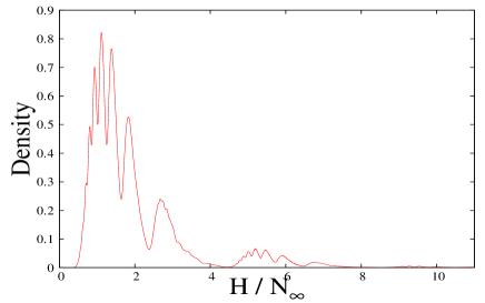
In the previous section we derived the distribution of $r_{j}$; from that we easily obtain the distribution for $H_{t}=1/F_{t}$ as follows. First, for each value of $d_{t}$ (the degree of the root node), we compute the distribution of $F_{t}$. The delta function part of this distribution (at $F_{t}=0$) is removed and the remaining distribution if rescaled to have norm 1. This corresponds to enforcing the constraint that the absorbing node is on the infinite component of the Erdös-Rényi graph (the part of the distribution of $F_{t}$ which gives zero flux corresponds to being on a finite component). Second, the distribution of $H_{t}=1/F_{t}$ is extracted: call it $\mu_{d_{t}}(H_{t})$. Finally, given all the distributions $\mu_{d_{t}}$ ($1\leq d_{t}<\infty$), the distribution of hitting times $H$ at random nodes is obtained by averaging the $\mu_{d_{t}}$ with their respective weights:

$$\mu(H)=\sum_{d_{t}=1}^{\infty}\frac{\mu_{d_{t}}\left(H_{t}\right)P(d_{t})(1-\Delta^{d_{t}})}{\sum_{j=1}^{\infty}P(j)(1-\Delta^{j})}$$ (12)

An example of such a distribution is shown in Fig. 2 when $\langle d\rangle=4$. Furthermore, the distribution of $H$ also gives the distribution of first passage times since at large $N$, for each value of $H$, the first passage time $n$ is distributed as $\exp{(-n/H)}$.

Figure 3: (Color online) Mean hitting times divided by $N_{\infty}$ for Erdös-Rényi graphs in the limit of large graphs, as a function of mean node degree $c=\langle d\rangle$. $N_{\infty}$ is the size of the “infinite” component, $N_{\infty}\approx(1-\Delta)N$ for graphs of $N$ nodes.

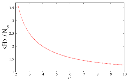
Finally, to obtain the mean hitting time $\langle H\rangle$, it is enough to compute the mean of the distribution of $H$. We have done so and show in Fig. 3 the resulting values, normalized by $N_{\infty}$, as a function of the mean degree of the graphs. At large $\langle d\rangle$, the ratio converges to $1$ with $O(1/\langle d\rangle)$ corrections: one recovers the dense graph result. Also, the behavior is very smooth and we find that it differs from the value when the degree does not fluctuate (the case of random $d$-regular graphs) also by $O(1/\langle d\rangle)$.

VII Validation of the tree approach

Figure 4: (Color online) Plot comparing numerical simulation with analytical results. The x axis shows the size of the largest connected component of the graph, the y axis shows the mean hitting time for such a component.

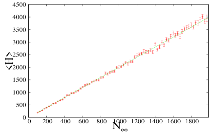
One of the key assumptions in the derivation of our formulas is that, since the graphs under consideration are locally tree-like, quantities such as the return probability can be computed by replacing the graphs by trees with the same statistics for the node degrees. There are certain systems where such an approach can be demonstrated to be exact in the large graph limit Aldous (2001), but unfortunately in most cases one has no such a proof. To see whether the tree approach might be exact (for large graphs) for the mean hitting times, we have computed by simulation the actual values for random graphs without resorting to any approximation. These values can then be compared to the theoretical predictions, in particular in the large graph size limit.

Fig. 4 shows the mean hitting times on the largest connected component of an Erdös-Rényi graph with mean degree $\langle d\rangle=4$. The estimation from Eq. (12) (based on the tree approach) is compared with values obtained from a numerical simulation in which we followed the probability vector $\mathbf{v}^{(n)}$ as in Eq. (6). For each randomly generated graph of size $N$, we numerically calculated the mean hitting time for a randomly chosen absorbing node $t$ on its largest connected component (whose size is $N_{\infty}$). The mean hitting times were then averaged over multiple graphs. The error bars are shown as well. We found that the values $\langle H\rangle/N_{\infty}$ determined from the simulations tend towards their large $N$ limit rather fast and that this limit is compatible with our analytical result, the relative difference being compatible with a $O(1/N)$ convergence. The same conclusion also holds in the context of random $d$-regular graphs (cf. Eq. (2)). In sum, the agreement of the theoretically predicted values with the results from numerical simulations gives some credence to the claim that the tree approach is exact in the large $N$ limit.

VIII Discussion and conclusion

We considered random walks on random graphs, focusing on two quantities: the distribution of hitting times and the probability that a walker will return to its starting point in a finite time. (The hitting time is the mean of first passage times.) By using the local tree approach Aldous (2001); Mézard et al. (2002), we were able to calculate analytically the large $N$ behavior of these quantities on two families of random graphs. We found non-trivial distributions having self-similar features associated with the discrete nature of possible neighborhoods of a node. Finally, we compared the calculated results with numerical simulations and found excellent agreement, justifying the tree approach which assumes that the loops in these graphs can be treated by appropriate boundary conditions on infinite trees.

Acknowledgments— We thank Satya Majumdar for enlightening discussions. This work was supported by the Sixth European Research Framework (proposal number 034952, GENNETEC project). The LPTMS is an Unité de Recherche de l’Université Paris-Sud associées au CNRS.

References

- Hughes (1996) B. Hughes, Random Walks and Random Environments (Clarendon Press, Oxford, 1996).
- Bouchaud and Georges (1990) J.-P. Bouchaud and A. Georges, Phys. Rep. 195, 127 (1990).
- Montroll and Shuler (1979) E. Montroll and K. Shuler, Proceedings of the National Academy of Sciences 76 (12), 6030 (1979).
- Newman (2005) M. Newman, Social Networks 27, 39 (2005).
- Noh and Rieger (2004) J. Noh and H. Rieger, Phys. Rev. Lett. 92, 118701 (2004).
- Benichou et al. (2005) O. Benichou, M. Coppey, M. Moreau, P. Suet, and R. Voituriez, Phys. Rev. Lett. 94, 198101 (2005).
- Feller (1950) W. Feller, An introduction to probability theory and its applications (John Wiley and sons, New York, NY, 1950).
- Redner (2001) S. Redner, A Guide to First-Passage Processes (Cambridge University Press, Cambridge, 2001).
- Lovász (1993) L. Lovász, in Paul Erdös is Eighty (Combinatorics, 1993).
- Bollobás (2001) B. Bollobás, Random Graphs (Cambridge University Press, Cambridge, 2001).
- Erdös and Rényi (1959) P. Erdös and A. Rényi, Publ. Math. Debrecen 6, 290 (1959).
- Chung et al. (2003) F. Chung, L. Lu, and V. Vu, Proceedings of the National Academy of Sciences 100, 6313 (2003).
- Sood et al. (2005) V. Sood, S. Redner, and D. Ben-Avraham, J. Phys. A 38, 109 (2005).
- Baronchelli and Loreto (2006) A. Baronchelli and V. Loreto, Phys. Rev. E 73, 026103 (2006).
- Biroli and Monasson (1999) G. Biroli and R. Monasson, J. Phys. A 32, L255 (1999).
- Semerjian and Cugliandolo (2002) G. Semerjian and L. F. Cugliandolo, J. Phys. A 35, 4837 (2002).
- Wormald (1999) N. Wormald, in Surveys in Combinatorics (Cambridge University Press, 1999), pp. 239–298.
- Aldous (2001) D. J. Aldous, Probability Theory and Related Fields 18(4), 381 (2001), math.PR/0010063.
- Mézard et al. (2002) M. Mézard, G. Parisi, and R. Zecchina, Science 297, 812 (2002).