Abstract A new expression for the characteristic function of log-spot in Heston model is presented. This expression more clearly exhibits its properties as an analytic characteristic function and allows us to compute the exact domain of the moment generating function. This result is then applied to the volatility smile at extreme strikes and to the control of the moments of spot. We also give a factorization of the moment generating function as product of Bessel type factors, and an approximating sequence to the law of log-spot is deduced.

Keywords Heston volatility model, Characteristic function, Extreme strikes, Bessel random variables.

Mathematics Subject Classification (2000) 91B28, 60H10, 60E10

JEL Classification G13, C65

1 Introduction

The first surprising fact about the Heston stochastic volatility model (Heston [11]) is that the characteristic function of log-spot is computable and has a nice expression in terms of elementary functions; its deduction had enormous merit. The second thing, and still more fascinating, is that such characteristic function is analytic, that means (see Lukacs [16, chapter 7] for an equivalent definition and the main properties of analytic characteristic functions) there is a function $\Psi(z)$ of the complex variable $z$, analytic in a neighborhood of 0, such that

$${\mathbb{E}}[e^{iuX_{t}}]=\Psi(iu)$$

for $u$ (real) in a neighborhood of 0, where $X_{t}$ is log-spot at time $t$.

The fact that a characteristic function is analytic has important consequences, and we here exploit some of them. However, the standard form of writing the Heston characteristic function hides the analycity property and difficults its utilization. So we first give a new expression of the characteristic function, but more importantly, we use that the analycity property is equivalent that the random variable has (real) moment generating function in a neighborhood of the origin: there is $\varepsilon>0$ such that

$$M(u)={\mathbb{E}}[e^{uX_{t}}]<\infty,\ -\varepsilon<u<\varepsilon.$$

In that case, the function $M(u)$ is a real analytic function in $(-\epsilon,\epsilon)$ and the main properties of the characteristic function can be studied through $M(u)$, which is a real function, and in general much simpler to analyze.

As a consequence of the study of the moment generating function we obtain the domain of that function and we give a numerical simple procedure to compute the poles of the characteristic function in its strip of convergence. This has several practical consequences and we apply it to the computation of the smile wings parameters in the formula given by Lee [14]. We also apply these results to the assessment of the moments of a particular model; such study is complementary of the one of Andersen and Piterbarg [2].

The second contribution of this paper is that we factorize the moment generating function of log-spot. This allows us to identify a Bessel type densities as the building blocks of the log-spot. This result has interesting applications. For example, it allows us to construct a sequence of random variables converging in law to log-spot. On the other hand, for a certain combinations of the parameters, log-spot $X_{t}$ is a sum of independent non-centered $\chi^{2}$ random variables, and we can identify $X_{t}$ as a member of the non-homogeneous second Wiener chaos (see Janson [13, chapter 6]); this agrees with the intuition that for some parameters, the stochastic volatitlity, given by a CIR model (Cox et al. [3]), has the law of the sum of the squares of a finite number of independent Ornstein-Uhlenbeck processes, that are in the second Wiener chaos, and such property is transferred to $X_{t}$.

The paper is organized as follows. First we deduce the moment generating function and the characteristic function of log-spot; as far as we know, these expressions are new. Both can be obtained manipulating the expressions obtained by Dufresne [6] or the standard expressions of the characteristic functions (see for example, Gatheral [9] or Albrecher et al. [1]), however we prefer to give a new deduction from scratch since our procedure is quite general and can be applied to other problems. In Section 3, we obtain the domain of the moment generating function. In Section 4, we give some applications. Finally, in Section 5, using techniques of complex analysis, the moment generating function of log-spot is factorized. The analysis of the factors allows us to identify them as moment generating functions of Bessel type random variables, and to construct a sequence of random variables that converges in law to log spot. In the Appendix we review some facts on moment generating function of a random variables and we put technical details of the proofs.

2 The Heston model

The Heston model [11] is defined by the system of stochastic differential equations

$$\left.\begin{aligned} dS_{t}&=\mu S_{t}\,dt+S_{t}\sqrt{V_{t}}\,dZ(t)\\ dV_{t}&=a(b-V_{t})\,dt+c\sqrt{V_{t}}\,dW(t)\end{aligned}\right\}$$ (1)

with initial conditions $S_{0}=s_{0}>0$ and $V_{0}=v_{0}\geq 0$, where $a,\,b>0$ and $c\in{\mathbb{R}}-\{0\}$ are constants, and $W$ and $Z$ are two standard correlated Brownian motions, $\langle Z,W\rangle_{t}=\rho t,$ for some $\rho\in[-1,1].$ The process $V_{t}$ is a Feller diffusion (Feller [7]) or, in the financial literature, a CIR model (Cox et al. [3]). The parameter $a$ is called the the mean reversion factor, $b$ is called the long term volatility and it is also written $V_{\infty}$, and $c$ is called the vol-of-vol. Write

$$X_{t}=\log S_{t}-\mu\,t.$$

By the Itô formula,

$$dX_{t}=-\frac{1}{2}V_{t}\,dt+\sqrt{V_{t}}\,dZ_{t},$$

with initial condition $X_{0}=x_{0}=\ln s_{0}$. Thus, we will consider the system

$$\left.\begin{aligned} dX_{t}&=-\frac{1}{2}V_{t}\,dt+\sqrt{V_{t}}\,dZ_{t}\\ dV_{t}&=a(b-V_{t})\,dt+c\sqrt{V_{t}}\,dW(t)\end{aligned}\right\}$$ (2)

2.1 The moment generating function of $\boldsymbol{X_{t}}$

First, we check that $X_{t}$ (indeed $(X_{t},V_{t})$) has moment generating function, and later we deduce its expression as the solution of a (real) PDE obtained from Itô formula.

For every $u,v\in{\mathbb{R}}$, the random variable $e^{uX_{t}+vV_{t}}$ is positive, so we can compute its expectation but it can be infinite. Write

$$Z_{t}=\rho W(t)+\sqrt{1-\rho^{2}}W^{\prime}(t),$$

where $W^{\prime}$ is a Brownian motion independent of $W$, and use the habitual trick

$$g(u,v,t):={\mathbb{E}}\big{[}e^{uX_{t}+vV_{t}}\big{]}={\mathbb{E}}\Big{[}{\mathbb{E}}\big{[}e^{uX_{t}+vV_{t}}/W^{\prime}(s),\ 0\leq s\leq t\big{]}\Big{]}.$$

We obtain

$$g(u,v,t) =\exp\big{\{}x_{0}u-\frac{uv_{0}\rho}{c}-\frac{u\rho abt}{c}\big{\}}$$

$$\cdot{\mathbb{E}}\Big{[}\exp\Big{\{}\big{(}v+\frac{\rho u}{c}\big{)}V_{t}+\big{(}\frac{u^{2}}{2}-\frac{u}{2}-\frac{\rho^{2}u^{2}}{2}+\frac{ua\rho}{c}\big{)}\int_{0}^{t}V_{s}\,ds\Big{\}}\Big{]}.$$

Note that the coefficient of $\int_{0}^{t}V_{s}\,ds$ is the equation of a parabola in $u$ through the origin, so if $u$ is near zero, that coefficient should be also near zero. Since both $V_{t}$ and $\int_{0}^{t}V_{s}\,ds$ have moment generation function (see Dufresne [5]) it follows that the expectation is finite for $(u,v)$ in a neighborhood of $(0,0)$. Fix $T>0$. Applying the Itô formula to $\exp\{uX_{t}+vV_{t}\}$ and taking expectations, we have

$$g(u,v,t) =e^{ux_{0}+vv_{0}}+vab\int_{0}^{t}g(u,v,s)\,ds+\Big{(}-\frac{u}{2}+\frac{u^{2}}{2}+\frac{v^{2}c^{2}}{2}+uv\rho c-va\Big{)}\int_{0}^{t}\frac{\partial g(u,v,s)}{\partial v}\,ds,$$

where we have used the property of the moment generating function

$$\frac{\partial g(u,v,s)}{\partial v}={\mathbb{E}}\big{[}e^{uX_{s}+vV_{s}}V_{s}\big{]}$$

Differentiating with respect to $t$, we get

$$\frac{\partial g(u,v,s)}{\partial t}-p(u,v)\frac{\partial g(u,v,t)}{\partial v}=abvg(u,v,t),$$

where

$$p(u,v)=-\frac{u}{2}+\frac{u^{2}}{2}+\frac{v^{2}c^{2}}{2}+uv\rho c-va.$$

This equation has a unique solution that is

$$g(u,v,t)=\Bigg{(}\frac{p\big{(}u,\phi(u,v,t)\big{)}}{p(u,v)}\Bigg{)}^{ab/c^{2}}\exp\big{\{}ux_{0}+\phi(u,v,t)v_{0}-\frac{abt\rho u}{c}+\frac{a^{2}bt}{c^{2}}\big{\}},$$

where

$$P(u) =\sqrt{(a-\rho cu)^{2}+c^{2}(u-u^{2})},$$

$$\gamma(u,v) =-2\arctan\!{\rm h}\big{(}(c^{2}v+c\rho u-a)/P(u)\big{)}/P(u)$$

$$\varphi(u,v,t) =-\frac{\rho u}{c}+\frac{a}{c^{2}}-\frac{1}{c^{2}}P(u)\tanh\Big{(}P(u)\big{(}t+\gamma(u,v)\big{)}/2\Big{)}.$$

For $v=0$, we get the moment generating function of $X_{t}$, $M_{t}(u)$; when there is no confusion we will suppress the subindex $t$ and write $M(u)$. After some tedious manipulations, $M(u)$ can be written as

$$M(u) ={\mathbb{E}}\Big{[}\exp\big{\{}uX_{t}\big{\}}\Big{]}$$

$$=\exp\{x_{0}u\}\ \bigg{(}\frac{e^{(a-c\rho u)t/2}}{\cosh(P(u)t/2)+\big{(}a-c\rho u)\sinh(P(u)t/2)/P(u)}\bigg{)}^{2ab/c^{2}}$$

$$\qquad\cdot\exp\bigg{\{}-v_{0}\,\frac{(u-u^{2})\sinh(P(u)t/2)/P(u)}{\cosh(P(u)t/2)+\big{(}a-c\rho u\big{)}\sinh(P(u)t/2)/P(u)}\bigg{\}},$$ (3)

where

$$P(u)=\sqrt{(a-\rho cu)^{2}+c^{2}(u-u^{2})}.$$

Remark 2.1.

Formula (2.1) coincides with the one that can be deduced from the joint Laplace-Mellin transformation of $S_{t},V_{t},\int_{0}^{t}V_{s}\,ds$ given by Dufresne [6, Theorem 12].

2.2 The characteristic function of $\boldsymbol{X_{t}}$

For $z$ complex, consider the function

$$\Phi(z)= \exp\{x_{0}z\}\ \bigg{(}\frac{e^{(a-c\rho z)t/2}}{\cosh(P(z)t/2)+(a-c\rho z)\sinh(P(z)t/2)/P(z)}\bigg{)}^{2ab/c^{2}}$$

$$\qquad\cdot\exp\bigg{\{}-v_{0}\ \frac{(z-z^{2})\sinh(P(z)t/2)/P(z)}{\cosh(P(z)t/2)+(a-c\rho z)\sinh(P(z)t/2)/P(z)}\bigg{\}}.$$ (4)

Write $p(z)=(a-\rho cz)^{2}+c^{2}(z-z^{2})$ the second degree polynomial within $P(z)$. Since $p(0)=a^{2}>0$, using standard techniques of complex analysis, we see that $\Phi(z)$ is well defined and analytic in a neighborhood of $0$. Obviously, $\Phi(u)=M(u)$ on a (real) neighborhood of 0. Then (see the Appendix, Proposition A.1, and Section 5), the characteristic function of $X_{t}$ is $\Phi(iu)$. Explicitly, for $u\in{\mathbb{R}}$,

$$\varphi(u)={\mathbb{E}}[e^{iuX_{t}}]=\Phi(iu) =\exp\{ix_{0}u\}\ \bigg{(}\frac{e^{at/2}}{\cosh(dt/2)+\xi\sinh(dt/2)/d}\bigg{)}^{2ab/c^{2}}$$

$$\qquad\cdot\exp\bigg{\{}-v_{0}\,\frac{(iu+u^{2})\sinh(dt/2)/d}{\cosh(dt/2)+\xi\sinh(dt/2)/d}\bigg{\}},$$ (5)

where

$$d =d(u)=P(iu)=\sqrt{(a-c\rho iu)^{2}+c^{2}(iu+u^{2})},$$

$$\xi =\xi(u)=a-c\rho ui.$$

After some computations we arrive to the formula of Albrecher et al. [1]

$$\varphi(u)=\exp\{ix_{0}u\}\exp\Big{\{}\frac{ab}{c^{2}}\Big{(}(\xi-d)t-2\log\frac{1-ge^{-dt}}{1-g}\Big{)}\Big{\}}\,\exp\Big{\{}\frac{v_{0}}{c^{2}}(\xi-d)\frac{1-e^{-dt}}{1-ge^{-dt}}\Big{\}},$$ (6)

where

$$g=g(u)=\frac{\xi-d}{\xi+d}.$$

Of course, formula (2.2) looks more complex than the compact (6). However, when one recovers from the shock, one realizes that the former is easier to handle that the latter.

2.3 Inversion of Heston model and some comments on the parameters

We will say that a process $S=\{S_{t},\ t\in[0,T]\}$ is a Heston type process, and we write $S\sim{\cal HP}_{\mathbb{P}}(a,b,c,\rho,s_{0},v_{0},\mu)$ if $S_{t}$ verifies a system (2) with some stochastic volatility $V_{t}$. When there is no confusion with the underlying probability $\mathbb{P}$ we will omit it.

Recent results of del Baño [4] show that if $S\sim{\cal HP}_{\mathbb{P}}(a,b,c,\rho,s_{0},v_{0},\mu)$, $a>c\rho$, then

$$S^{-1}\sim{\cal H}_{{\mathbb{Q}}}(a-c\rho,ab/(a-c\rho),c,-\rho,s_{0}^{-1},v_{0},-\mu),$$ (7)

where ${\mathbb{Q}}$ is the probability given by

$$\frac{d{\mathbb{Q}}}{d\mathbb{P}}=e^{X_{T}}.$$

To prove that property it is needed to work with the whole process $S$. However, an easy verification can be done using the moment generating function (2.1). We will use this property in Section 3 to compute the values of ${\mathbb{E}}[\exp\{uX_{t}\}]$ for negative values of $u$.

It can also be proved that

$${\cal HP}_{\mathbb{P}}(a,b,c,\rho,s_{0},v_{0},\mu)\sim{\cal HP}_{\mathbb{P}}(a,b,-c,-\rho,s_{0},v_{0},\mu).$$

Again, it is needed to consider the process to prove this equality, but a check is deduced from the expression of the moment generating function (2.1). So, without loss of generality we will assume from now on that $c>0$.

3 The domain of the moment generating function

In this section we deduce the domain of the moment generating function (2.1); this deduction is not direct since we obtained $M(u)$ not by the computation of the expectation ${\mathbb{E}}[e^{uX_{t}}]$ but by an indirect way. So, we only know that the moment generating function coincides with the function given in the right hand side of (2.1) in a neighborhood of zero. However, as stated by Lemma 3.3 below, since the function is analytic, we are in safe land. In the first subsection, using this idea we do a first study of the moment generating function. Later, in the second subsection we work with the analytic continuation of the function in the right hand side of (2.1).

3.1 Preliminary study of the domain of the moment generating function

The main ingredient of the moment generating function given in (2.1) is

$$f(u):=\cosh(P(u)t/2)+(a-c\rho u)\,\frac{\sinh(P(u)t/2)}{P(u)},$$ (8)

where

$$P(u)=\sqrt{(a-\rho cu)^{2}+c^{2}(u-u^{2})}.$$

Write

$$p(u):=(a-\rho cu)^{2}+c^{2}(u-u^{2}).$$ (9)

When $\rho\neq\pm 1$, $p(u)$ represents a parabola with leading coefficient $c^{2}(\rho^{2}-1)\leq 0$, and for $u=0$, we have $a^{2}>0$. So, it is an inverted parabola with real roots, $u_{-}<0<u_{+}$, given by

$$u_{\pm}=\frac{c-2a\rho\pm\sqrt{4a^{2}+c^{2}-4ac\rho}}{2c(1-\rho^{2})}.$$ (10)

When $\rho=-1$, then

$$p(u)=a^{2}+c(c+2a)u,$$

is a straight line with positive slope that intersects the horizontal axis at $u_{-}=-a^{2}/(c(c+2a))<0,$ and we write $u_{+}=\infty$.

Similarly, for $\rho=1$, $p(u)$ degenerates in the straight line

$$p(u)=a^{2}+c(c-2a)u,$$

and the slope can be negative, postitive or zero or negative, and

• When $2a>c$, then $u_{-}=-\infty$.

• When $2a<c$, then $u_{+}=\infty$.

• When $2a=c$, then $u_{-}=-\infty$ and $u_{+}=\infty$.

Thus, for every $\rho\in[-1,1]$, we have that $p(u)\geq 0$ on $[u_{-},u_{+}]$, hence the function $f(u)$ is well defined and analytic in such (possible infinite) interval. Denote by $D(X_{t})$ the domain of $M(u)$,

$${D}(X_{t})=\big{\{}u\in{\mathbb{R}}:\ M(u)={\mathbb{E}}\big{[}e^{uX_{t}}\big{]}<\infty\big{\}}.$$

In principle (see Lemma 3.3 bellow) $M(u)$ is defined in the subinterval of $[u_{-},u_{+}]$ between the biggest negative zero and the smallest positive zero of $f(u)$. Next proposition summarizes the study of such zeroes in that interval.

Proposition 3.1.

For every $t>0$, and $\rho\in[-1,1]$ there is the inclusion $[u_{-},1]\subset D(X_{t})$. Moreover,

1. When $a\geq c\rho$ (in particular, for every $\rho<0$), then for all $t>0$, the function $f(u)$ has no zeroes in $[u_{-},u_{+}]$, and consequently, $[u_{-},u_{+}]\subset D(X_{t}).$ (Except for $\rho=1$ and $c=2a$).

2. When $a<c\rho$, write $t_{0}=2/(c\rho u_{+}-a)\geq 0$

   1. If $t<t_{0}$, then $[u_{-},u_{+}]\subset D(X_{t})$, and $f(u)$ has no zeroes in $[u_{-},u_{+}]$.

   2. If $t\geq t_{0}$, then $f(u)$ has no zeroes in $[u_{-},1]$, and has one and only one zero in $(1,u_{+}]$.

3. When $\rho=1$ and $a=2c$, then $D(X_{t})=\big{(}-\infty,1/(1-e^{-at})\big{)}$.

Remark 3.2.

1. The cases $\rho=\pm 1$ are specially important. We stress that

   1. For $\rho=-1$, we are always in case $1$ and $u_{+}=\infty$.

   2. For $\rho=1$, when $a\geq c$, we are in case 1 (except if $a=2c$). For $a<c$ we are in case 2; however, if $a<c<2a$, then $u_{+}=\infty$, and we have $t_{0}=0$, and thus we are in case (ii) for all $t>0$.

2. From the preceding proposition it follows that ${\mathbb{E}}[S_{t}]<\infty$ for every $a,b,c>0$ and $\rho\in[-1,1]$. Moreover, when $\mu=0$, by construction, $\{S_{t},\,t\in[0,T]\}$ is an exponential local martingale, that is a positive supermartingale, see Revuz and Yor [17, pages 148 and 149], and

   $${\mathbb{E}}[S_{t}]=M(1)=e^{x_{0}},$$

   so $\{S_{t},\,t\in[0,T]\}$ is a true martingale. This was proved by Andersen and Piterbarg [2, Proposition 2.5] using the Feller explosion criteria and Girsanov Theorem.

3. As a continuation of the preceding point, we should remark that $\{S_{t},\,t\in[0,T]\}$ is not always a square integrable martingale. This can cause some problems. See Subsection 4.2.

3.2 Computation of the abscissæ of convergence of the moment generating function

When there is no root of $f(u)$ in $[1,u_{+}]$ the domain $D(X_{t})$ is larger than $[u_{-},u_{+}]$ (in particular, when $a>\rho c$). To carry out this study, we need more properties of the moment generating function. Consider an arbitrary random variable $X$, with moment generating function $M_{X}(u)$, and domain $D_{X}=\big{\{}u\in{\mathbb{R}}:\ M_{X}(u)<\infty\big{\}}$. Remember that $D_{X}$ is a interval of ${\mathbb{R}}$ (finite or infinite, open or closed from one side or the other, that always include the origin, and it may be just $\{0\}$), and $M_{X}$ is analytic in the interior of ${D_{X}}$. The left (respectively right) extreme of ${D_{X}}$ is called the left (resp. right) abscissa of convergence, and plays a major role. The following property is well known, but since it is key in this paper, we stress it. We give the property for the right abscissa of convergence, and a similar statement is true for the left abscissa,

Lemma 3.3.

Let $X$ a random variable such that there is a neighborhood of zero included in $D_{X}$. Assume that $(r,s]\subset{D_{X}}$, and that there is an analytic function $h:(p,q)\to{\mathbb{R}}$ such that

1. $(r,s]\subset(p,q)$.

2. $M_{X}(u)=h(u)$,  for  $u\in(r,s]$.

Then $M_{X}=h$ on $(p,q)$. Moreover, if   $\lim_{u\nearrow q}h(u)=\infty,$ then the right–abscissa of convergence of $M_{X}$ is the point $q$.

Proof.

Denote the interior of $D_{X}$ by $(\alpha,\beta)$. If $\beta=\infty$, by analytic continuation, $M_{X}=h$ on $(r,q)$. Consider $\beta<\infty$, so $\beta$ is the finite right–abscissa of convergence. Then the function $M_{X}$ has a singularity at $\beta$ (see the Appendix, Proposition A.2) Thus, $s\neq\beta$, because $M_{X}(s)=h(s)$ and $h$ is analytic in $s$. Hence, $\beta>s$. In the same way, $\beta<q$ is contradictory, then $\beta\geq q$ and by analytic continuation, $M_{X}=h$ on $(r,q)$. The second part of the Lemma is obvious. $\qquad\square$

Now we apply the preceding lemma to the moment generating function of the log-spot, $M(u)$. When the function $f(u)$ given in (8) has no zeros in $[1,u_{+}]$, since

$$\lim_{u\searrow u_{-}}M(u)<\infty\qquad\text{and}\qquad\lim_{u\nearrow u_{+}}M(u)<\infty,$$

by Lemma 3.3, the domain of $M(u)$, $D(X_{t})$, is bigger than $[u_{-},u_{+}]$ Then, to assess more carefully that domain, consider the function $\cosh\sqrt{x}$, for $x>0$. Its Taylor expansion is

$$\cosh\sqrt{x}=\sum_{n=0}^{\infty}\frac{x^{n}}{(2n)!}.$$

The series on the right defines an entire function, say $L_{1}(x)$. However, when $x<0$, that series coincides with the Taylor expansion of $\cos\sqrt{-x}$. Hence, $L_{1}(x)$ is an entire function that, when written as the composition of elementary functions, has different expression according to whether $x>0$ or $x<0$, that is

$$L_{1}(x)=\begin{cases}\cosh\sqrt{x},&\text{if $x\geq 0$},\\ \\ \cos\sqrt{-x},&\text{if $x\leq 0$}.\end{cases}$$

In a similar way, the function $(\sinh\sqrt{x})/\sqrt{x},\ x>0,$ can be analytically continuated to negative numbers as $(\sin\sqrt{-x})/\sqrt{-x},\ x<0$.

Denote by $u_{-}^{*}\geq-\infty$ the left abscissa of convergence of $M(u)$ and by $u_{+}^{*}\leq\infty$ the right abscissa. Put

$$\widetilde{P}(u)=\sqrt{-p(u)}.$$

For $u\in(u_{-}^{*},u_{-})$ or $u\in(u_{+},u_{+}^{*})$, by Lemma 3.3 the moment generating function is

$$M(u) =\exp\{x_{0}u\}\ \bigg{(}\frac{e^{(a-c\rho u)t/2}}{\cos(\widetilde{P}(u)t/2)+\big{(}a-c\rho u)\sin(\widetilde{P}(u)t/2)/\widetilde{P}(u)}\bigg{)}^{2ab/c^{2}}$$

$$\qquad\cdot\exp\bigg{\{}-v_{0}\,\frac{(u-u^{2})\sin(\widetilde{P}(u)t/2)/\widetilde{P}(u)}{\cos(\widetilde{P}(u)t/2)+\big{(}a-c\rho u\big{)}\sin(\widetilde{P}(u)t/2)/\widetilde{P}(u)}\bigg{\}}.$$ (11)

In that expression, the main part is the function

$$\widetilde{f}(u):=\cos(\widetilde{P}(u)t/2)+(a-c\rho u)\frac{\sin(\widetilde{P}(u)t/2)}{\widetilde{P}(u)}.$$ (12)

Both $f$ and $\widetilde{f}$ are defined in disjoint sets, and can be combined in a new function

$$F(u)=\begin{cases}f(u),&\text{if $u\in[u_{-},u_{+}]$,}\\ \\ \widetilde{f}(u),&\text{if $u<u_{-}$ or $u>u_{+}$,}\end{cases}$$ (13)

that is analytic in ${\mathbb{R}}$. See Figure 1 for a plot of that function.

Figure 1: Plot of $F(u)$. The points $u_{-}^{*}$ and $u_{+}^{*}$ are the abcissæ  of convergence of $M(u)$.

Then, to find the right abscissa of convergence, we need to find the zero of the function $f(u)$ in $[1,u_{+}]$, and if there is no zero, then to find the smallest zero $u>u_{+}$ of $\widetilde{f}(u)$. Note also that the real zeroes of $\widetilde{f}(u)$ are the real solutions of the equation (see Figure 2)

$$\tan(\widetilde{P}(u)t/2)=-\frac{\widetilde{P}(u)}{a-c\rho u}.$$ (14)

(Except when $a/c\rho=k\pi/2$ for some natural number $k$).

Figure 2: Solid line: Plot of $\tanh\big{(}P(u)t/2\big{)}$, for $u\in[u_{-},u_{+}]$ or $\tan\big{(}\widetilde{P}(u)t/2\big{)}$ in the complementary. Dashed line: Plot of $-P(u)/(a-\rho cu)$ or $-\widetilde{P}(u)/(a-\rho cu)$.

For the left abscissa of convergence we need to look for the biggest solution $u<u_{-}$ of $\widetilde{f}(u)=0$, or, equivalently, to work with equation (14).

In order to give a bound for the abscisses of convergence, denote by $\alpha_{\pm 1}$ the solutions of the equation

$$p(u)=-\frac{4\pi^{2}}{t^{2}},$$

that for all $t>0$ are real and $\alpha_{-1}<u_{-}$ and $\alpha_{+1}>u_{+}$. Also put $\beta_{\pm 1}$ the solutions of $p(u)=-2\pi^{2}/t^{2}.$ Consider the following cases:

1. If $a>\rho c$, then $u_{+}^{*}\in(u_{-},\alpha_{+1})$. This can be deduced from the consideration that the image of the function $\tan(\widetilde{P}(u)t/2)$ on that interval is ${\mathbb{R}}$, and the properties of the function in the right hand side of (12). The only case not clear is when $a/(c\rho)=\pi/2$, due to the fact that $-{\widetilde{P}(u)}/(a-c\rho u)$ has a vertical asymptote at $u=\beta_{1}$; this case is studied by direct inspection.

2. If $a<\rho c$, then remember that $f(1)>1$, and, on the other hand,

   $$\widetilde{f}(\beta_{+1})=(a-c\rho\beta_{+1})2/\pi<0,$$

   because $\beta_{+1}>1$ and $\rho>0$. So $F(u)$ has at least one root in $(1,\beta_{+1})$.

Joining these comments with Proposition 3.1 we have

Theorem 3.4.

With the above notations,

1. If $a>\rho c$, the right abscissa of convergence $u_{+}^{*}$ is the smallest zero $u>u_{+}$ of $\widetilde{f}(u)=0$, and $u_{+}^{*}\in(u_{+},\alpha_{+1})$. (Except for $\rho=1$ and $a=2c$).

2. If $a=\rho c$, the right abscissa of convergence is $u_{+}^{*}=1$.

3. If $a<\rho c$, let $t_{0}=2/(c\rho u_{+}-a)\geq 0$.

   1. If $t<t_{0}$, then $u_{+}^{*}$ is smallest zero $u>u_{+}$ of $\widetilde{f}(u)=0$, and $u_{+}^{*}\in(u_{+},\beta_{+1})$.

   2. If $t\geq t_{0}$, then $u_{+}^{*}$ is the zero of $f(u)$ in $(1,u_{+}]$.

4. In every case, the left abscissa of convergence, $u_{-}^{*}$ is the biggest zero $u<u_{-}$ of $\widetilde{f}(u)=0$ and $u_{-}^{*}\in(\alpha_{-1},u_{-})$.

Remark 3.5.

1. When $a>\rho c$ the inversion formula (7) can be used to compute $u^{*}_{-}$ in terms of $u^{*}_{+}$ of the inverted model. Specifically,

   $$u^{*}_{-}(a,c,\rho,t)=-u^{*}_{+}(a-c\rho,c,-\rho,t)+1.$$

2. This theorem gives a direct procedure to invert the formulas of Andersen and Pitebarg [2, Proposition 3.1].

4 Applications

In this section we present some applications of the exact knowledge of the abcissæ  of convergence of the moment generating function of log-spot.

4.1 The smile at extreme strikes

One of the motivations for the study of the abcissæ  of convergence of the moment generating function of log-spot in the Heston model in this work is the outstanding result of Roger Lee ([14]) where an explicit relation is found between the assymptotic behaviour of the volatility smile and these abcissæ. This can be of interest in designing sensible smile interpolation and extrapolation schemes as has been shown by Gatheral [8]. In the case under consideration, that of the Heston dynamics, if $u_{+}^{*}$ and $u^{*}_{-}$ are the abcissæ  of convergence of log-spot, then according to Lee [14] the asymptotic behaviour of the Heston smile for expiry $T$ as the strike $K$ goes to infinity is $\sigma(K)\approx\sqrt{\beta_{R}\ln(K)/{T}}$ where $\beta_{R}\in[0,2]$ is defined by

$$\frac{1}{2\beta_{R}}+\frac{\beta_{R}}{8}-\frac{1}{2}=u_{+}^{*}-1.$$

Likewise the behaviour as $K$ approaches zero is $\sigma(K)\approx\sqrt{-\beta_{L}\ln(K)/{T}}$ where $\beta_{L}\in[0,2]$ is defined by

$$\frac{1}{2\beta_{L}}+\frac{\beta_{L}}{8}-\frac{1}{2}=-u^{*}_{-},$$

As an example, consider market data for a one year equity smile $\rho=-90\%,\,a=2,\,c=80\%,\,b=15\%^{2}$ and $t=1$. The calculations outlined above yield $u_{+}^{*}=37.43$ and $u_{-}^{*}=-3.21$. By Roger Lee’s formulas above this implies the behaviour of the smile wings is ruled by

$$\beta_{R}=0.01\quad\text{and}\quad\beta_{L}=0.13$$

where, as expected, the smile at low strikes has a larger coefficient. These numbers can be of use to design an extrapolation scheme for the Heston smile in extreme strikes where the numerical integration breaks down.

4.2 The importance of second order moment of spot in stochastic volatility models

The moments of spot and the abcissæ  of convergence of log-spot are related because

$$u_{+}^{*}=\sup\{u\in\mathbb{R}:\ {\mathbb{E}}[S_{t}^{u}]<\infty\}\quad\text{and}\quad u_{-}^{*}=\inf\{u\in\mathbb{R}:\ {\mathbb{E}}[S_{t}^{u}]<\infty\}.$$ (15)

So, if $u_{+}^{*}<2$, then the second order moment of spot is infinite. This can cause problems in pricing certain standard European derivatives, as the next couple of examples show.

1. Pricing an FX performance note. Consider a performance note that pays Euros on the performance of the EUR/USD exchange rate. This is a contract that pays the following amount in Euros at expiry $T$

$$\text{Payoff}(EURUSD_{T})=\text{Notional}_{EUR}\left(\frac{EURUSD_{T}}{EURUSD_{0}}-1\right)\qquad EUR$$

The notation should be self explanatory: $EURUSD_{t}$ is the EUR/USD exchange rate at time $t$ and $t=0$ is today. By the standard martingale methods the price of a derivative product is simply its discounted expectation, this might (and does) lead naive market participants to price such a transaction as

$$\text{Present Value}=Df_{T}^{EUR}\text{Notional}_{EUR}\left(\frac{F_{T}}{EURUSD_{0}}-1\right)\qquad EUR$$

where we have used the fact that the risk neutral expectation of spot is the forward $F_{T}$, and write $Df_{T}^{EUR}$ for the relevant discount factor. Unfortunately this approach is flawed since EUR/USD is the price in US Dollars of one Euro and in the equations above we are basing a Euro payment on this quantity. Its correct price can be derived by noting that its payout in Dollars is

$$\text{Payoff}(EURUSD_{T})=\text{Notional}_{EUR}\left(\frac{EURUSD_{T}}{EURUSD_{0}}-1\right)\cdot EURUSD_{T}\qquad USD$$

and here we can apply the martingale methods to yield

Present Value $$= Df_{T}^{USD}\text{Notional}_{EUR}\mathbb{E}\left(\left(\frac{EURUSD_{T}}{EURUSD_{0}}-1\right)\cdot EURUSD_{T}\right)$$

$$= Df_{T}^{USD}\text{Notional}_{EUR}\left(\frac{\mathbb{E}\left(EURUSD_{T}^{2}\right)}{EURUSD_{0}}-F_{T}\right)$$

an expression that involves the second moment of spot. A model that has an infinite second moment for spot (and these things do appear in practice) will price such a contract at infinity.

2. LIBOR paid in arrears. A similar type of deal occurs in the fixed income derivatives market under the name of LIBOR paid in arrears. Normally LIBOR is a rate fixed on a certain date $T_{1}$ and paying at a later date $T_{2}$. A simple contract depending on LIBOR is a FRA (Forward Rate Agreement) whose payout is defined by

$$\delta(L-K)\qquad\text{paid at time }T_{2}$$

here L is the LIBOR rate which fixes at $T_{1}<T_{2}$ and $\delta$ is the day-count fraction which is approximately $T_{2}-T_{1}$. If we use the $T_{2}$-forward measure, the value of such a contract is simply the discounted expectation $\delta P(0,T_{2})\mathbb{E}(L-K)$ where $P(0,T_{2})$ is the $T_{2}$-discount bond. Given that $L_{t}=\frac{1}{\delta}(P(t,T_{1})-P(t,T_{2}))/P(t,T_{2})$ is the ratio of a tradeable instrument by the numeraire, we know it is a martingale in the $T_{2}$-forward measure and since $L_{T_{1}}$ is simply the LIBOR rate, the price of our FRA is

$$P(0,T_{2})\delta\mathbb{E}(L-K) = P(0,T_{2})\delta\mathbb{E}(L_{T_{1}}-K)$$ (16)

$$= P(0,T_{2})\delta(L_{0}-K)$$ (17)

where $L_{0}=\frac{1}{\delta}(P(0,T_{1})-P(0,T_{2}))/P(0,T_{2})$ is the so-called forward LIBOR rate, the rate that makes the FRA have zero value. A LIBOR in-arrears transaction is based on LIBOR paid at the wrong time, its payout being

$$\delta(L-K)\qquad\text{paid at time }T_{1}$$

A naive idea to price these transactions is to simply discount the by the forward discount factor $P(0,T_{2})/P(0,T_{1})$ which of course just affects equation (16) by a multiplicative factor and does not alter the fair forward price $L_{0}$. This is wrong because the expectation of $L$ is no longer the forward LIBOR in the $T_{1}$-forward measure which this approach implicitly uses. Some banks have been arbitraged in the past by using this naive approach. As in the case of the EURUSD note described above, if we convert the payment to a payment at time $T_{2}$ then we can use the expectations in the $T_{2}$-forward measure, the payout at time $T_{2}$ is simply the accrued amount

$$\delta(1+\delta L)\cdot(L-K)\qquad\text{paid at time }T_{2}$$

and its price will be

$$P(0,T_{2})\delta\mathbb{E}\left((1+\delta L)\cdot(L-K)\right)$$

and so the fair strike is strictly larger than the FRA rate

$$L_{0}+\delta\frac{\mathbb{V}ar(L)}{1+\delta L_{0}}$$

an expression that involves the second moment of the LIBOR rate.

4.3 Dependence of the abscissæ of convergence on the time.

In this subsection we assume that $\mu=0$, so $\{S_{t},\,t\in[0,T]\}$ is a martingale. In order to study the dependence of the abcissæ  of convergence on the time, we denote by $u_{+}^{*}(t)$ and $u_{-}^{*}(t)$ the abcissæ  for $X_{t}$. The following proposition is a general property of a positive martingale.

Proposition 4.1.

Consider $0\leq t<t^{\prime}\leq T$. Then

$$u_{+}^{*}(t)\geq u_{+}^{*}(t^{\prime})\quad\text{and}\quad u_{-}^{*}(t)\leq u_{-}^{*}(t^{\prime}).$$

Proof.

Fix for a moment $r\geq 1$. The function $\phi(x)=x^{r}$ on $(0,\infty)$ is convex. Since $\{S_{t},\,t\in[0,T]\}$ is a positive martingale, assuming enough integrablity, $\{S_{t}^{r},\,t\in[0,T]\}$ is a submartingale. Hence, for $t<t^{\prime}$,

$${\mathbb{E}}[S^{r}_{t}]\leq{\mathbb{E}}[S^{r}_{t^{\prime}}].$$

For $\epsilon>0$, such that $u_{+}^{*}(t^{\prime})-\varepsilon>1$, we have that

$${\mathbb{E}}[S^{u_{+}^{*}(t^{\prime})-\varepsilon}_{t}]\leq{\mathbb{E}}[S^{u_{+}^{*}(t^{\prime})-\varepsilon}_{t^{\prime}}]<\infty,$$

and this implies $u_{+}^{*}(t)\geq u_{+}^{*}(t^{\prime})-\varepsilon$, and the result follows from (15).

For the negative abscissa, just observe that for $r<0$, the same function $\varphi(x)=x^{r}$ on $(0,\infty)$ is also convex, and apply the same reasoning. $\square$

For Heston model, we can be more precise. From the bounds given in Theorem 3.4, it is deduced the behaviour of the abcissæ for $t\to\infty$

$$\lim_{t\to\infty}u_{+}^{*}(t)=u_{+}\quad\text{and}\quad\lim_{t\to\infty}u_{-}^{*}(t)=u_{-},$$

and for $t\to 0$:

$$\lim_{t\to 0}u_{+}^{*}(t)=\infty\quad\text{and}\quad\lim_{t\to 0}u_{-}^{*}(t)=-\infty.$$

A plot of these funcions is given is Figure 3.

Figure 3: Solid line: Plot of $u^{*}_{+}(t)$. Dashed line: Plot of $u^{*}_{-}(t)$.

4.4 The effective vol-of-vol and the effective mean reversion

It is interesting that in formula (10) the numbers $u_{\pm}$ only depend on the quotient $\omega:=a/c$. Expressed in terms of this parameter we have, for $\rho\neq\pm 1$,

$$u_{\pm}=\frac{1-2\omega\rho\pm\sqrt{4\omega^{2}+1-4\omega\rho}}{2(1-\rho^{2})}.$$

Intuitively, this is a consequence of the fact that the parameter $a$ (mean reversion) dampens the stochastic volatility whereas $c$ (vol-of-vol) increases it, thus operating in opposite directions. However the parameters $u_{\pm}$ correspond to the moments at infinite time, and in general the relative strength of the parameters $a$ and $c$ in flattening the smile is time dependent. We propose to call this parameter the effective mean reversion factor, and its inverse $c/a$ the effective vol-of-vol. The use of this parameter simplifies the study of $u_{\pm}$ for $\rho$ near $\pm 1$:

$$\lim_{\rho\to-1}u_{-}=-\frac{\omega^{2}}{2\omega+1}\quad\text{and}\quad\lim_{\rho\to-1}u_{+}=\infty,$$

and

$$\lim_{\rho\to 1}u_{-}=\begin{cases}\dfrac{\omega^{2}}{2\omega-1},&\text{if\ $\omega\ <1/2$}\\ \\ -\infty,&\text{if \ $\omega\geq 1/2$}\end{cases}\qquad\text{and}\qquad\lim_{\rho\to 1}u_{+}=\begin{cases}\infty,&\text{if \ $\omega\leq 1/2$}\\ \\ \dfrac{\omega^{2}}{2\omega-1},&\text{if \ $\omega\ >1/2$}\end{cases}$$

5 Factorization of the moment generating function of $\boldsymbol{X_{t}}$.

In this section we will work exclusively with the random variable $X_{t}$ for $t>0$ fixed, and the time $t$ will be considered a parameter. Denote by ${\cal HL}(a,b,c,\rho,x_{0},v_{0},\mu,t)$ the law of $X_{t}$, that is, a probability on ${\mathbb{R}}$ that has the moment generating function given by (2.1). Observe that for all $\lambda>0$,

$${\cal HL}(\lambda a,\lambda b,\lambda c,\rho,x_{0},\lambda v_{0},\mu,t/\lambda)={\cal HL}(a,b,c,\rho,x_{0},v_{0},\mu,t).$$

In particular,

$${\cal HL}(a,b,c,\rho,x_{0},v_{0},\mu,t)={\cal HL}(at/2,bt/2,ct/2,\rho,x_{0},v_{0}t/2,\mu,2).$$

Since we are interested in a property true for all parameters, it suffices to prove that property for arbitrary $a,b,c,\rho,x_{0},v_{0},\mu,$ and $t=2$. So, in all proofs, we will take this value of $t$.

In this section we use some powerful theorems of complex variable analysis that we apply to the complex moment generating function

$$\Phi(z)= \exp\{x_{0}z\}\ \bigg{(}\frac{e^{(a-c\rho z)t/2}}{\cosh(P(z)t/2)+(a-c\rho z)\sinh(P(z)t/2)/P(z)}\bigg{)}^{2ab/c^{2}}$$

$$\qquad\cdot\exp\bigg{\{}-v_{0}\ \frac{(z-z^{2})\sinh(P(z)t/2)/P(z)}{\cosh(P(z)t/2)+(a-c\rho z)\sinh(P(z)t/2)/P(z)}\bigg{\}},$$ (18)

defined in a neighborhood of zero, introduced in Subsection 2.2. We will consider separately the different factors of this function. and at a later stage, we will combine them.

5.1 The entire component

Write

$$F(z)=\cosh(P(z)t/2)+(a-c\rho z)\,\frac{\sinh(P(z)t/2)}{P(z)}.$$ (19)

Recall that

$$p(z)=(a-\rho cz)^{2}+c^{2}(z-z^{2})$$

and $P(z)=\sqrt{p(z)}.$ As in Subsection 3.2, but now in the complex plane, define the entire functions by the power series

$$L_{1}(z)=\sum_{n=0}^{\infty}\frac{z^{n}}{(2n)!},$$ (20)

and

$$L_{2}(z)=\sum_{n=0}^{\infty}\frac{z^{n}}{(2n+1)!}.$$ (21)

We note that at each $z$,

$$L_{1}(z)=\cosh\sqrt{z}\quad\text{and}\quad L_{2}(z)=\frac{1}{\sqrt{z}}\,\sinh\sqrt{z},$$

independently of the branch of the square root. Indeed, in every neighborhood that does not include zero, the previous relations are true fixing an arbitrary branch of the square root. However, in the whole ${\mathbb{C}}$, the functions $L_{1}$ and $L_{2}$ are defined by the power series and not as a composition of $\cosh z$ or $\sinh z$ and a particular branch of $\sqrt{z}$. We consider the extension of $F(z)$ to an entire function using the functions $L_{1}(z)$ and $L_{2}(z)$. Note that both $L_{1}(z)$ and $L_{2}(z)$ take real values on ${\mathbb{R}}$, and that $F(z)$ restricted to ${\mathbb{R}}$ coincides with the function $F(u)$ defined in (13).

The first interesting property of $F(z)$ is that it has all the zeroes real and simple. This can be deduced from a deep theorem of Lucic [15, Theorem 1] who proves that all the singularities of the (complex) characteristic function of $X_{t}$ are purely imaginary. In Appendix B there is an alternative proof of this property. Specifically, we prove that

Proposition 5.1.

The zeroes of $F(z)$ are all real and simple.

Using the Hadamard representation theorem (see the Appendix, Theorem B.1), we deduce the following representation of $F(z)$.

Theorem 5.2.

Let $\{a_{n}(t),\,n\geq 1\}$ be the zeroes of $F(z)$. Then

$$F(z)=e^{at/2}e^{\nu(t)z}\prod_{n=1}^{\infty}\Big{(}1-\frac{z}{a_{n}(t)}\Big{)}\exp\Big{\{}\frac{z}{a_{n}(t)}\Big{\}},$$ (22)

where $\nu(t)\in{\mathbb{R}}$.

Remark 5.3.

The number $\nu(t)$ in (22) is determinated by

$$F(1)=\cosh\big{(}|a-\rho c|t/2\big{)}+\text{sign}\,\{a-\rho c\}\,\sinh\big{(}|a-\rho c|t/2\big{)}=e^{at/2}e^{\nu(t)}\prod_{j=1}^{\infty}\Big{(}1-\frac{1}{a_{j}(t)}\Big{)}\exp\Big{\{}\frac{1}{a_{j}(t)}\Big{\}}.$$ (23)

Remark 5.4.

In all of this Section we exclude the case $\rho=1$ and $a=2c$ because the moment generating function simplifies and has only one pole in that case. Then the factorization is trivial.

5.2 The meromorphic component

Now we will deal with the other factor of the function $\Phi(z)$ given in (5),

$$\frac{(z-z^{2})\sinh(P(z)t/2)/P(z)}{\cosh(P(z)t/2)+(a-c\rho z)\sinh(P(z)t/2)/P(z)}.$$

Write

$$G(z)=\frac{(1-z)\sinh(P(z)t/2)/P(z)}{\cosh(P(z)t/2)+(a-c\rho z)\sinh(P(z)t/2)/P(z)},$$

where, as above, the function is extended to ${\mathbb{C}}$ using the entire functions $L_{1}(z)$ and $L_{2}(z)$. The function $G(z)$ is meromorphic with simple poles at the roots of $F(z)$. Using a theorem of Mittag-Leffler, see the Apendix, Theorem B.2, we prove

Theorem 5.5.

Let $\{a_{n}(t),\,n\geq 1\}$ be the zeroes of $F(z)$, ordered in the following way: $0<|a_{1}(t)|\leq|a_{2}(t)|\leq\cdots$ . Then, for $z\neq a_{n}(t)$, $\forall n\geq 1$,

$$G(z)=\frac{1}{2a}(1-e^{-at})-z\sum_{n=1}^{\infty}\frac{b_{n}(t)}{a_{n}(t)^{2}(1-z/a_{n}(t))},$$ (24)

where $b_{n}(t)>0$, and $\sum_{n}\frac{b_{j}(t)}{a_{j}^{2}(t)}<\infty$, and the series converges uniformly in every compact set included in the disc $|z|<|a_{1}|$.

5.3 Factorization of the moment generating function of $\boldsymbol{X_{t}}$

We return to the real moment generating function $M(u)$. Combining the results of the two preceding subsections we have that the moment generating function $M(u)$ given in (2.1) can be factorized as (we abreviate $a_{n}(t)$ and $b_{n}(t)$ to $a_{n}$ and $b_{n}$ for a moment), for $u\in(-|a_{1}|,\,|a_{1}|),$

$$M(u)=\exp\{du\}\,\prod_{n=1}^{\infty}\Big{(}1-\frac{u}{a_{n}}\Big{)}^{-2ab/c^{2}}\exp\Big{\{}-\frac{2ab}{c^{2}}\frac{u}{a_{n}}+v_{0}\frac{u^{2}b_{n}}{a_{n}^{2}(1-u/a_{n})}\Big{\}},$$

where $d$ is a parameter to be defined later. Each exponential can be written as

$$c_{n}u+\frac{g_{n}u}{1-u/a_{n}}.$$

where

$$c_{n}=-(v_{0}b_{n}+2ab/c^{2})/a_{n}\quad\text{and}\quad g_{n}=v_{0}b_{n}/a_{n}.$$ (25)

Remark 5.6.

When $4ab/c^{2}=k$ is a natural number, we can identify the moment generating function as the one given by Janson [13, Theorem 6.2], each eigenvalue with multiplicity $k$. That means, for such parameters, $X_{t}$ is in the (non-homogeneous) second Wiener chaos. It is well known that for such combination of parameters the CIR model has the law of a sum of the squares of $k$ independent Ornstein-Uhlenbeck processes, and this fact has been used for many applications. See, for example, Grasselli and Hurd [10] and the references therein.

On the other hand, for $u$ in a neighborhood of 0, the moment generating function of each factor can be written as

$$N_{j}(u)=e^{c_{n}u}\Big{(}1-\frac{u}{a_{n}}\Big{)}^{-2ab/c^{2}}\exp\Big{\{}\frac{g_{n}u}{1-u/a_{n}}\Big{\}},$$

where $a_{n}\cdot g_{n}>0$.

Proposition 5.7.

For $\xi>0$ and $\zeta,\gamma\in{\mathbb{R}}$, such that $\zeta\cdot\gamma>0$, the function

$$N(u)=\big{(}1-u/\gamma\big{)}^{-\xi}\exp\Big{\{}\frac{\zeta u}{1-u/\gamma}\Big{\}}$$

for $u$ in a neighborhood of 0, is the moment generating function of an absolutely continuous random variable with probability density function

$$h(x)=\frac{1}{2}\bigg{(}\frac{x}{\zeta}\bigg{)}^{\tau}\exp{\{-(x+\zeta)\gamma\}}I_{2\tau}(2\gamma\sqrt{\zeta x}){\bf 1}_{(0,\infty)}(x),\ \text{if}\ \zeta,\gamma>0,$$

or

$$h(x)=\frac{1}{2}\bigg{(}\frac{x}{\zeta}\bigg{)}^{\tau}\exp{\{-(x+\zeta)\gamma\}}I_{2\tau}(-2\gamma\sqrt{\zeta x}){\bf 1}_{(-\infty,0)}(x),\ \text{if}\ \zeta,\gamma<0,$$

where $\tau=(\xi-1)/2$ and $I_{2\tau}$ is the Bessel function of index $2\tau$.

Proof.

For $\zeta,\gamma>0,$ the moment generating function $N(u)$ corresponds to the law of $Y_{1/(2\gamma)}$ for a Bessel process

$$Y_{t}=\zeta+2\xi t+2\int_{0}^{t}\sqrt{Y_{s}}\,dW_{s}.$$

See Revuz-Yor [17, Chapter 11]. Its density is also given in Revuz-Yor [17, page 441].

For $\zeta,\gamma<0,$ consider the random variable $Y$ defined above with parameters $-\zeta$ and $-\gamma$, and let $Y^{\prime}=-Y$. Its moment generating function is

$$M_{Y^{\prime}}(u)=M_{Y}(-u)=\big{(}1-u/\gamma\big{)}^{-\xi}\exp\Big{\{}\frac{\zeta u}{1-u/\gamma}\Big{\}}.$$

Its density is $h_{Y}(-x)$, where $h_{Y}$ is the density of $Y$. And the result follows.  $\square$

Return to the factors $N_{j}(u)$. The term $e^{c_{n}u}$ is a translation factor of the random variable considered above, so $N_{j}(u)$ corresponds to a random variable with density $h_{n}(x-c_{n}),$ where $h_{n}$ is the probability density function given in Proposition 5.7.

Finally, the product of characteristic functions of absolutely continuous laws with densities $k_{1}$ and $k_{2}$ corresponds to the convolution $k_{1}\star k_{2}$:

$$k_{1}\star k_{2}(x)=\int_{-\infty}^{+\infty}k_{1}(y)k_{2}(x-y)\,dy.$$

Denote by $\bigstar_{j=1}^{n}k_{j}$ the product $k_{1}\star\cdots\star k_{n}$, that is defined without ambiguity because the convolution product is associative and commutative.

With all these ingredients we construct a sequence of random variables that converges in law to $X_{t}$. In general, the convergence in law does not imply the convergence of the corresponding probability density functions. However, from a practical point of view, this fact does not matter.

Theorem 5.8.

The sequence of laws with densities $\bigstar_{j=1}^{n}\widetilde{h}_{j}$ converges to the law of $X_{t}+d(t)$, where $\widetilde{h}_{n}(x)=h_{n}(x-c_{n})$, and $h_{n}$ is the probability density function given in Proposition 5.7, with parameters

$$\xi=2ab/c^{2},\,\gamma=a_{n}(t),\,\zeta=g_{n}(t),$$

where

1. $a_{n}(t)$ are the roots of the function $F(u)$.

2. $$b_{n}(t)=\frac{4p\big{(}a_{n}(t)\big{)}\big{(}1-a_{n}(t)\big{)}}{tp^{\prime}\big{(}a_{n}(t)\big{)}p\big{(}a_{n}(t)\big{)}-4c\rho p\big{(}a_{n}(t)\big{)}-p^{\prime}\big{(}a_{n}(t)\big{)}(a-c\rho a_{n}(t))\big{(}(a-c\rho a_{n}(t))t+2\big{)}}.$$

3. $c_{n}(t)$ and $g_{n}(t)$ are given in equation (25).

4. $$d(t)=x_{0}-\frac{\rho abt}{c}-\frac{2ab\nu(t)}{c^{2}}-\frac{v_{0}(1-e^{-at})}{2a}.$$

5. $\nu(t)$ is given in formula (23).

Conclusions

We have presented a new expression of the characteristic function of log-spot in Heston model that shows its good analytical properties and that facilitates its study. Through an analysis of the corresponding moment generating function, we give numerical formulas to obtain the abscissæ of convergence, that have interesting applications. As examples we considered the computation of the parameters describing the asymptotic behaviour of the volatility smile for extreme strikes, and the verification that the model has enough moments to price wing dependent deals. Another application may be the possibility of assessing the stability of the moments in a calibration of a Heston model.

In the second part of the paper, we factorized the moment generating function as an infinite product of Bessel type moment generating function. This gives a new insight of the Heston model, showing its complexity, and its relationship with Ornstein-Uhlenbeck processes. Further, each factor can be inverted, and a sequence of random variables that converges in law to log-spot can be deduced. Though such sequence is not easy to manage, because it relies on the computation of the roots of a (real) function and other parameters, and the convolution of densities involving Bessel functions. The fact that all computations are real can open the possibility of alternative methods to the numerical inversion of the characteristic function that are currently used by practitioners.

Appendix

Appendix A. Complex and real moment generating function

For a sake of completeness, we recall some of the properties of the complex and real moment generating function of an arbitrary random variable $X$. We follow Hoffmann-Jørgensen [12]. The complex function

$$M_{\mathbb{C}}(z)={\mathbb{E}}[e^{zX}],$$

defined on the set

$${D}_{\mathbb{C}}=\big{\{}z\in{\mathbb{C}}:\ {\mathbb{E}}\big{[}\big{|}e^{zX}\big{|}\big{]}<\infty\big{\}},$$

is called the complex moment generating function (cmgf from now on) of $X$. We will denote by $\mathrel{\mathop{\kern 0.0ptD}\limits^{\raisebox{-5.0pt}{\text{\scriptsize$\circ$}}}}_{\mathbb{C}}$ the interior of ${D}_{\mathbb{C}}$. The restriction of $M_{\mathbb{C}}(z)$ to the real numbers is the moment generating function (mgf)

$$M_{\mathbb{R}}(u)={\mathbb{E}}[e^{uX}],$$

defined on the set

$$D_{\mathbb{R}}=\big{\{}u\in{\mathbb{R}}:\ {\mathbb{E}}\big{[}e^{uX}\big{]}<\infty\big{\}}.$$

(we also put $\mathrel{\mathop{\kern 0.0ptD}\limits^{\raisebox{-5.0pt}{\text{\scriptsize$\circ$}}}}_{\mathbb{R}}$ by the interior of $D_{\mathbb{R}}$). For the present purposes it is convenient to maintain the double notation with the subindices ${\mathbb{R}}$ and ${\mathbb{C}}$. Since for $z\in{\mathbb{C}}$ and $a\in{\mathbb{R}}$, $|\exp\{az\}|=\exp\{a\,\Re z\},$ we deduce that

$${D}_{\mathbb{C}}=\big{\{}z\in{\mathbb{C}}:\ \Re z\in{D}_{\mathbb{R}}\big{\}}=D_{\mathbb{R}}+i\,{\mathbb{R}}.$$

The most important property of both $M_{\mathbb{C}}(z)$ and $M_{\mathbb{R}}(u)$ is that they are analytic functions on the interior of its domains, and that the Taylor expansion of $M_{\mathbb{C}}(z)$ in a point of the real axis has the same (real) coefficients than $M_{\mathbb{R}}(u)$. Again, here, it is useful to introduce a double notation for the neighborhoods. For $u\in{\mathbb{R}}$ and $r>0$, we denote by $B_{\mathbb{R}}(u,r)$ the neighborhood centered at $u$ with radius $r$, and for $z\in{\mathbb{C}}$, $B_{\mathbb{C}}(z,r)$ is the neighborhood in ${\mathbb{C}}$. If $D_{\mathbb{R}}\neq\{0\}$, the cmgf $M_{\mathbb{C}}$ (respectively the mgf $M_{\mathbb{R}}$) is analytic in $\mathrel{\mathop{\kern 0.0ptD}\limits^{\raisebox{-5.0pt}{\text{\scriptsize$\circ$}}}}_{\mathbb{C}}$ (resp. $\mathrel{\mathop{\kern 0.0ptD}\limits^{\raisebox{-5.0pt}{\text{\scriptsize$\circ$}}}}_{\mathbb{R}}$). and for $z_{0}\in\mathrel{\mathop{\kern 0.0ptD}\limits^{\raisebox{-5.0pt}{\text{\scriptsize$\circ$}}}}_{\mathbb{C}}$ there is $r>0$ such that

$$M_{\mathbb{C}}(z)=\sum_{n=0}^{\infty}\,\frac{{\mathbb{E}}\big{[}e^{z_{0}X}X^{n}\big{]}}{n!}\,(z-z_{0})^{n},\quad\forall z\in B_{\mathbb{C}}(z_{0},r),$$ (26)

and for $u_{0}\in\mathrel{\mathop{\kern 0.0ptD}\limits^{\raisebox{-5.0pt}{\text{\scriptsize$\circ$}}}}_{\mathbb{R}}$ there is $r>0$ such that

$$M_{\mathbb{R}}(u)=\sum_{n=0}^{\infty}\,\frac{{\mathbb{E}}\big{[}e^{u_{0}X}X^{n}\big{]}}{n!}\,(u-u_{0})^{n},\quad\forall u\in B_{\mathbb{R}}(u_{0},r).$$ (27)

In particular, if $0\in\mathrel{\mathop{\kern 0.0ptD}\limits^{\raisebox{-5.0pt}{\text{\scriptsize$\circ$}}}}_{\mathbb{R}}$, then $X$ has finite moments of all orders and, writing

$$m_{n}=E[X^{n}],\ n\geq 1,$$

we have that for some $r>0$,

$$M_{\mathbb{C}}(z)=\sum_{n=1}^{\infty}\frac{m_{n}}{n!}\,z^{n},\ \forall z\in B_{\mathbb{C}}(0,r),$$

and

$$M_{\mathbb{R}}(u)=\sum_{n=1}^{\infty}\frac{m_{n}}{n!}\,u^{n},\ \forall u\in B_{\mathbb{R}}(0,r).$$

Moreover,

$${\mathbb{E}}[X^{n}]=M^{(n)}(0).$$

Proposition A.​ 1.

Assume that there is a function $\Phi(z)$ of the complex variable $z$ analytic in a neighborhood of   0 such that

$$M_{\mathbb{R}}(u)=\Phi(u),$$

for $u$ in a (real) neighborhood of 0. Then the function $\Phi(z)$ can be analytically continuated in a strip that includes the imaginary axis, and the characteristic function of $X$ is

$${\mathbb{E}}[iuX_{t}]=\Phi(iu),\ \forall u\in{\mathbb{R}}.$$

Proof. Since $M_{\mathbb{R}}(u)$ and $M_{\mathbb{C}}(z)$ have the same Taylor coefficients in a neighborhood of 0, we have that $\Phi(z)=M_{\mathbb{C}}(z)$ in a complex neighborhood of 0. Since $M_{\mathbb{C}}(z)$ is analytic in $\mathrel{\mathop{\kern 0.0ptD}\limits^{\raisebox{-5.0pt}{\text{\scriptsize$\circ$}}}}_{\mathbb{C}}$, the function $\Phi$ can be continuated to that strip that includes the imaginary axis.  $\square$

Remember that $D_{\mathbb{R}}$ is an interval of ${\mathbb{R}}$ (it may be ${0}$), and the right extreme (respectively the left extreme) of $D_{\mathbb{R}}$ is called the right–abscissa (resp. the left–abscissa) of convergence.

Proposition A.​ 2.

Assume that $0\in\mathrel{\mathop{\kern 0.0ptD}\limits^{\raisebox{-5.0pt}{\text{\scriptsize$\circ$}}}}_{\mathbb{R}}$, and that the right-abscissa of convergence, $\beta$, (respectively the left-abscissa $\alpha$) is finite. Then $M_{\mathbb{R}}(u)$ has a singularity at $\beta$ (resp. $\alpha$).

Proof. When $X$ is positive, the cmgf coincides with the Laplace transform (except a change of sign on $z$) of the distribution function of $X$. By Widder [19, Theorem II.5b]), $M_{\mathbb{C}}(z)$ has a singularity at the real point $\beta$. From the fact that in the real axis both $M_{\mathbb{C}}$ and $M_{\mathbb{R}}$ have the same coefficients of the Taylor expansion, Widder’s proof can be translated to $M_{\mathbb{R}}$. For a general $X$, we can use the habitual technique of decomposing a bilateral Laplace transform as the addition of two unilateral ones (see Widder [19, page 237])).  $\square$

Appendix B. Proofs

Proof of Proposition 3.1

We have that $p(0)=a^{2}$ and $p(1)=(a-\rho)^{2}\geq 0,$ then, given the form or $p(u)$, it follows that $1\leq u_{+}$. Hence, the affirmation $[u_{-},1]\subset D(X_{t})$ is obtained from the other points of the proposition.

1. Consider the case $a\geq\rho c$, $\rho\neq\pm 1.$ A bit of algebra shows that $a-\rho cu_{-}>0$ and $a-c\rho u_{+}>0$. So the straightline $y=a-\rho cu$ is positive for $u\in[u_{-},u_{+}]$ (see Figure 4). Since $\cosh x\geq 1,\forall x\in{\mathbb{R}}$, and $\sinh x>0,\forall x>0$, it follows that $f(u)>0$ in $[u_{-},u_{+}]$. Note that if $a=\rho c$, then $u_{+}=1$.

Figure 4: Solid line: straightline $y=a-\rho cu$, case $a>\rho c$, for $\rho>0$. Dashed line: parabola $p(u)$

When $\rho=-1$, then $u_{-}=-a^{2}/(c(c+2a))<0,$ and it is trivial that $a+cu_{-}>0$. So the straithgtline $y=a+cu$ is positive for $u\geq u_{-}$, and hence $f(u)>0$ in $[u_{-},\infty)$.

When $\rho=1$, and $c\neq 2a$, then $u_{+}=a^{2}/(c(2a-c))$, and some calculations shows that in this case ($a\geq c)$, then

$$\frac{a}{c}\geq\frac{a^{2}}{c(2a-c)},$$

and hence, $a-cu_{+}\geq 0$. Then $a-cu\geq 0$ for all $u\leq u_{+}$, and it follows $f(u)>0$ in $(-\infty,u_{+}].$

2. Consider the case $a<\rho c$ (note that this implies $\rho>0$). Then $a-c\rho u_{-}>0$ and $a-c\rho\big{(}\frac{a}{c\rho}\big{)}=0$. So the straighline $y=a-c\rho u$ is positive for $u\in[u_{-},a/(c\rho)]$. Thus $f(u)$ has no zeroes in such interval. On the other hand, the real zeroes of $f(u)$ in $[u_{-},u_{+}]$ are the same of the ones corresponding to the function

$$1+\frac{a-c\rho u}{P(u)}\tanh(P(u)t/2),$$

because of the real hyperbolic cosine is never zero. For $u\geq a/(\rho c),$ and the bound $0<\tanh x<1$, for all $x>0$, we have

$$1+\frac{a-c\rho u}{P(u)}\tanh(P(u)t/2)>1+\frac{a-c\rho u}{P(u)},$$

and when $u\in[a/(\rho c),1]$, from $c^{2}u(1-u)\geq 0$ it is deduced that

$$1+\frac{a-c\rho u}{P(u)}\geq 0,$$

hence $f(u)>0$ also in $[a/(\rho c),1]$. Now, we analyze the behaviour of $f(u)$ for $u\in[1,u_{+}]$. Assume $\rho\neq 1$. From

$$\lim_{u\nearrow u_{+}}\frac{\sinh\big{(}P(u)t/2\big{)}}{P(u)t/2}=1.$$

it follows that

$$\lim_{u\nearrow u_{+}}f(u)=1+(a-c\rho u_{+})t/2.$$

Consider the straightline $y=a-c\rho u$. We have $y(0)=a$ and $y(1)=a-c\rho<0$, and since $u_{+}>1$, then $a-c\rho u_{+}<0$. Let $t_{0}=2/(c\rho u_{+}-a)>0.$

1. If $t<t_{0}$, from $(c\rho u_{+}-a)t_{0}/2=1$, then for all $u\in[1,u_{+}],$

   $$0<(c\rho u-a)t_{0}/2<1,$$

   and thus

   $$0<(c\rho u-a)t/2<1.$$

   Hence, $\forall u\in[1,u_{+}],$

   $$\frac{(c\rho u-a)t}{2}\ \frac{\sinh\big{(}P(u)t/2\big{)}}{P(u)t/2}<\frac{\sinh\big{(}P(u)t/2\big{)}}{P(u)t/2}\leq\cosh\big{(}P(u)t/2\big{)},$$

   because ${\sinh x}/{x}\leq\cosh x$. Then $f(u)>0.$

2. Let $t\geq t_{0}$. Then $\ f(1)>0$ and $f(u_{+})<0,$ and thus there is at least one zero of $f(u)$ in $[1,u_{+}].$ The fact that there is only one zero is proved in Section 5.

Finally, the case $\rho=1$ and $a<c$  or $a=2c$ are studied in a similar way. $\square$

Proof of the results of Section 5.

For easy reference, we recall here the two main theorems used in the proofs, expressed in the form that we need. The first one is the factorization Theorem of Hadamard (see, for example, Titchmarsch [18])

Theorem B.​ 1.

Let $F(z)$ an entire function, $F(0)\neq 0$, with roots $a_{1},\,a_{2},\dots,$ such that

$$\sum_{n}1/|a_{n}|^{2}<\infty.$$

Then $F$ can be represented as

$$F(z)=F(0)e^{Cz}\prod_{n}\Big{(}1-\frac{z}{a_{n}}\Big{)}e^{z/a_{n}}.$$

The second theorem is due to Mittag-Leffler (Titchmarsch [18, page 110])

Theorem B.​ 2.

Let $G(z)$ be a meromorphic function such all the poles are simple, denoted by $a_{1},\,a_{2},\dots,$ where $0<|a_{1}|\leq|a_{2}|\leq\cdots,$ and with residues at the poles $b_{1},\,b_{2}\dots$ respectively. Suppose that there is a sequence of closed contours $C_{n}$ such that $C_{n}$ includes $a_{1},\dots,a_{n}$ but no other poles, such that the minimum distance $R_{n}$ of $C_{n}$ to the origin tends to infinite with n, while the length of $C_{n}$ is $O(R_{n})$, and on $C_{n}$, $f(z)=o(R_{n})$. Then

$$G(z)=G(0)-z\sum_{n}\frac{b_{n}/a_{n}^{2}}{1-z/a_{n}}.$$

In order to prove Proposition 5.1 we need three lemmas.

Lemma B.​ 3.

For all $z\in{\mathbb{C}}$,

$$\big{|}\coth\sqrt{z}\big{|}\leq\sup_{|w|=\sqrt{|z|}}\big{|}\coth w\big{|},$$

and similarly for $\tanh\sqrt{z}$.

Proof.

Consider the formula

$$|\coth z|^{2}=\frac{\sinh^{2}x+\cos^{2}y}{\sinh^{2}x+\sin^{2}y}.$$ (28)

Write $z=r\,e^{i\theta}$ and choose an arbitrary branch of the square root, for example, take the principal one. Then

$$\big{|}\coth\sqrt{z}\big{|}^{2} =\frac{\sinh^{2}(\sqrt{r}\,\cos(\theta/2))+\cos^{2}(\sqrt{r}\,\sin(\theta/2))}{\sinh^{2}(\sqrt{r}\,\cos(\theta/2))+\sin^{2}(\sqrt{r}\,\sin(\theta/2))}$$

$$\leq\sup_{\phi\in[0,\,2\pi)}\frac{\sinh^{2}(\sqrt{r}\,\cos\phi)+\cos^{2}(\sqrt{r}\,\sin\phi)}{\sinh^{2}(\sqrt{r}\,\cos\phi)+\sin^{2}(\sqrt{r}\,\sin\phi)}$$

$$=\sup_{|w|=\sqrt{r}}\big{|}\coth w\big{|}^{2}.\quad\square$$

Lemma B.​ 4.

For every $\varepsilon>0$ there is $n_{0}\geq 1$ such that for $n\geq n_{0}$,

$$\sup_{|z|=(n+\frac{1}{2})\pi}|\coth z|<1+\varepsilon$$

and

$$\sup_{|z|=n\pi}|\tanh z|<1+\varepsilon.$$

Proof

From the formula (28) it is clear that $|\coth z|$ is the same for the points $z=x+iy,\,-x+iy,\ x-iy,\ -x-iy$. Hence, to bound $\coth z$ in the circle $\{z\in{\mathbb{C}}:\ |z|=(n+\frac{1}{2})\pi\}$ we can restrict ourselves to study the arc with $\Re z\geq 0$ i $\Im z\geq 0.$ (see the Figure 5 for $n=2$).

Figure 5: Arc $|z|=(n+\frac{1}{2})\pi,\ \Re z\geq 0,\ \Im z\geq 0$ for $n=2$.

Given the periodicity $\coth(z+k\pi i)=\coth z$, for all $k\in{\mathbb{Z}}$, it suffices to bound the translation to the strip $0\leq\Im z\leq\pi$ (see Figure 6 (a)). For $K$ big enough, for $n\geq n_{0}$ all translations are included in the shaded region $A_{K}\cup B_{K}$ of Figure 6 (b). Thus, it suffices to prove that for $K$ big enough, $\sup_{z\in A_{K}\cup B_{K}}|\coth z|<1+\varepsilon.$ For $z=x+iy\in A_{K}$, (that is, $x>K$), we have

$$|\coth z|^{2}=\frac{\sinh^{2}x+\cos^{2}y}{\sinh^{2}x+\sin^{2}y}\leq\frac{\sinh^{2}x+1}{\sinh^{2}x}=1+\frac{1}{\sinh^{2}x}\leq 1+\frac{1}{\sinh^{2}K},$$

that goes to 1 when $K\to\infty.$

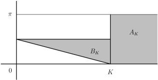
Figure 6: (a) Translation to the arc of Figure 5 to the strip $0\leq|\Im z|\leq\pi$. (b) The translation for all $n\geq n_{0}$ are included in the shadow region

Now we study the bound on the triangle $B_{K}$ of the Figure 6 (b). By the principle of the maximum, we need only to study the function on the border of $B_{K}$. On the vertical side, $z=K+iy,\ y\in[0,\pi/2]$, works the bound that we have found above. On the horizontal side, $z=x+i\frac{\pi}{2},\ x\in[0,K]$, by the formula (28),

$$|\coth z|^{2}=\frac{\sinh^{2}x}{\sinh^{2}x+1}\leq 1.$$

Finally, the hypotenuse is $z=x+iy$ with $y\in[0,\pi/2]$ i $x=-2Ky/{\pi}+K.$ For $y\in[\pi/4,\,\pi/2],$ we have that $\cos 2y\leq 0$, and by

$$|\coth z|^{2}=\frac{\cosh 2x+\cos 2y}{\cosh 2x-\cos 2y},$$

we deduce that

$$|\coth z|\leq 1.$$

For $y\in[0,\,\pi/4]$, we have $x\in[K/2,K]$, and again by (28) we obtain the bound.

To bound $|\tanh z|$ for $|z|=n\pi$ we do the same reductions as before, and use the relationship

$$\tanh z=\coth\big{(}z-i\frac{\pi}{2}\big{)},$$

to translate the bounds of $\coth z$ to $\tanh z$.  $\square$

We also need the properties of the contour determinated by the polynomial $p(z)$. For $d>0$ let $C_{d}$ be the contour

$$C_{d}=\{z\in{\mathbb{C}}:\,|p(z)|=d\},$$

and denote by $L_{d}$ its length and by $R_{d}$ the minimum distance from $L_{d}$ to the origin. See Figure 7

Lemma B.​ 5.

With the above notations, for $d$ big enough, $C_{d}$ is a homotopic to 0, $\lim_{d\to\infty}R_{d}=\infty,$ and $L_{d}\sim o(R_{d}^{2})$, when $d\to\infty$.

Proof

Since $p(z)$ is a second degree polynomial, there are two constants $K_{1},\,K_{2}>0$ such that for $|z|$ big enough,

$$K_{1}|z|^{2}\leq|p(z)|\leq K_{2}|z|^{2}.$$

It follows that for $d$ big enough, the circles with radius $d/K_{2}$ i $d/K_{1}$ bound lower and upper the contour $C_{d}$. This implies that $C_{d}$ is closed.

Figure 7: Contour $|p(z)|=d$, for $d$ big.

The polynomial $p(z)$ has real coefficients and has a positive and a negative root ($\rho\neq\pm 1$), and since the length of a contour does not change by translation, we can consider that $p(z)=z^{2}-a$, with $a>0$ (change also $d$ in order that the coefficient of $z^{2}$ is 1). Write $z=x+iy$; then the equation that determines $C_{n}$ is

$$(x^{2}+y^{2}+a)^{2}-4ax^{2}=d^{2}.$$

In polar coordinates, $x=r(\theta)\cos\theta$ and $x=r(\theta)\sin\theta$, the contour is given by

$$r^{4}(\theta)-2a\cos(2\theta)r^{2}(\theta)+a^{2}-d^{2},\ \theta\in[0,2\pi].$$

For $d$ big enough, we need only to consider the solution

$$r(\theta)=\sqrt{a\cos(2\theta)+\sqrt{a^{2}cos(4\theta)+d^{2}}},$$

that determines a curve clearly homotopic to 0. To compute the length $L_{d}$, by symmetry,

$$L_{d}=4\int_{0}^{\pi/2}\sqrt{r^{2}(\theta)+\big{(}r^{\prime}(\theta)\big{)}^{2}}\,d\theta.$$

We have $\lim_{d\to\infty}r(\theta)/d=0$ and $\lim_{d\to\infty}r^{\prime}(\theta)/d=0$, uniformly in $\theta\in[0,\pi/2]$, and the lemma follows.  $\square$

Proof of Proposition 5.1

Remember that we consider $t=2$. First, note that for $\rho\neq\pm 1$,

$$\lim_{z\to\infty}\frac{(a-c\rho z)^{2}}{(a-c\rho z)^{2}+c^{2}(z-z^{2})}=\frac{\rho^{2}}{\rho^{2}-1}.$$

Hence,

$$\lim_{z\to\infty}\Bigg{|}\frac{a-c\rho z}{P(z)}\Bigg{|}=\frac{|\rho|}{\sqrt{1-\rho^{2}}}.$$ (29)

Consider the following three cases:

Case 1. $|\rho|/{\sqrt{1-\rho^{2}}}>1.$

First step. The objective of this step is to prove that in the contour

$$C_{n}=\{z\in C:\,|p(z)|=(n+0.5)^{2}\pi^{2}\},$$

for $n$ big,

$$|\cosh P(z)|<\Big{|}(a-c\rho z)\frac{\sinh P(z)}{P(z)}\Big{|}.$$ (30)

Then, by Rouche Theorem, both functions $F(z)$ and $(a-c\rho z)\sinh(P(z))/P(z)$ have the same number of zeroes in $C_{n}$. To prove the inequality (30), take $\varepsilon>0$ such that $1<1+\varepsilon<|\rho|/{\sqrt{1-\rho^{2}}}.$ By Lemmas B3 and B4, for $n$ big enough, and $z\in C_{n}$, we have $|\coth P(z)|<1+\varepsilon,$ and apply the limit (29).

Second step. Study of the zeroes of $F(z)$. Assume that $\rho\neq 0$. The zeroes of $(a-c\rho z)\sinh(P(z))/P(z)$ are $z=a/(c\rho)$ and the zeroes of $\sinh(P(z))/P(z)$. We have that

$$\frac{\sinh P(z)}{P(z)}=\prod_{n=1}^{\infty}\Bigg{(}1+\frac{p(z)}{n^{2}\pi^{2}}\Bigg{)}.$$

Hence, the zeroes of this function are the roots of the second order polynomial

$$p(z)=-n^{2}\pi^{2},\ n=1,\,2,\dots,$$

that we denote by $\alpha_{\pm n}$; write also $u_{-}=\alpha_{-0}$ and $u_{+}=\alpha_{+0}$, in agreement with the notations of Section 3. They all are real and

$$\cdots\alpha_{-(n+1)}<\alpha_{-n}<\cdots\alpha_{-1}<\alpha_{-0}<0<\alpha_{+0}<\alpha_{+1}<\cdots<\alpha_{+n}<\alpha_{+(n+1)}<\cdots.$$

So, for $n$ big, $F(z)$ has $2n+1$ zeroes in $C_{n}$.

Now we count the number of real roots of $F(z)$ in $C_{n}$. Assume that $a>c\rho$ and $\rho>0$. We saw in the proof of Proposition 3.1 that $a/(c\rho)>u_{+}$, and assume that $a/(c\rho)\in(\alpha_{+k},\alpha_{+(k+1)})$ (the case $a/(c\rho)=\alpha_{+k}$ needs to be studied as a particular case). Then,

1. In each interval $(\alpha_{+n},\alpha_{+(n+1)})$, for $n=0,\dots k-1$, $F(u)=\widetilde{f}(u)$, where $\widetilde{f}(u)$ was defined in (12), and $\widetilde{f}(u)$ has one root. This is deduced because the roots of $\widetilde{f}(u)$ in such intervals are the solutions of

   $$\tan\widetilde{P}(u)=-\frac{\widetilde{P}(u)}{a-c\rho u}.$$

2. In $(\alpha_{+k},\alpha_{+(k+1)})$, $\widetilde{f}(u)$ has $2$ roots. This claim is proved, observing that $a-c\rho\,\alpha_{+k}>0$ and $a-c\rho\,\alpha_{+k}<0$, and the the curve $-\widetilde{P}(u)/(a-c\rho u)$ cuts two times the curve $\tan\widetilde{P}(u)$ in that interval.

3. In each $(\alpha_{-(n+1)},\alpha_{-n}),\ n\geq 0$, the function $\widetilde{f}(u)$ has one root. This is proved as in point (i).

All the other possibilities for $a,\,c$ and $\rho$ are discussed in a similar way, and we obtain that $F(z)$ has at least $2n+1$ real roots in $C_{n}$. So the Theorem follows.

Case 2. $|\rho|/{\sqrt{1-\rho^{2}}}<1.$ Here use the contours

$$C_{n}^{\prime}=\{z\in C:\,|p(z)|=n^{2}\pi^{2}\},$$

and prove that for $z\in C^{\prime}_{n},$ ($n$ big),

$$\Big{|}(a-c\rho z)\frac{\sinh P(z)}{P(z)}\Big{|}<|\cosh P(z)|.$$ (31)

and finish the proof as in Case 1.

Case 3. $\rho=\pm\sqrt{2}/2$. Write $\rho_{n}=\rho+1/n$, for $n\geq 4$, and let $F_{n}$ be the function $F$ with $\rho$ changed by $\rho_{n}$. We have $F_{k}(z)\to F(z)$ as $k\to\infty$, uniformly in every disc. By Hurwitz theorem (see Titchmarsch [18]), the roots of $F(z)$ in such disc are the limit points of the roots of $F_{k}(z)$ in the disc. So the roots of $F(z)$ are also real.  $\square$.

Proof of Theorem 5.2

In the proof of Proposition 5.1 we saw that for $n$ big, positive or negative, in each interval $(\alpha_{+n},\alpha_{+(n+1)})$ and $(\alpha_{-(n+1)},\alpha_{-n})$ there is one and only one root of $F(z)$, where

$$p(\alpha_{\pm n})=-n^{2}\pi^{2}.$$

Since $p(u)$ is a second degree polynomial, there are constants $K_{1},\,K_{2}>0$ such that for $|u|$ big enough,

$$K_{1}\,u^{2}\leq|p(u)|\leq K_{2}\,u^{2},$$

and then

$$\frac{1}{\sqrt{K_{2}}}n\pi\leq|\alpha_{\pm n}|\leq\frac{1}{\sqrt{K_{1}}}n\pi.$$ (32)

Hence,

$$\sum_{n}\frac{1}{a_{n}^{2}}<\infty\quad\text{and}\quad\sum_{n}\frac{1}{|a_{n}|}=\infty.$$

By Hadamard factorization Theorem B.1 we obtain the representation (22). $\square$

Remark B.​ 6.

An alternative way to prove the previous result is using that the order (as entire function) of $F(z)$ is less or equal to 1. This can be deduced from that fact that by the definitions (20) and (21)

$$|L_{j}(z)|\leq\cosh(\sqrt{|z|}),\ j=1,2,$$

and that the order of $L_{1}(z)$ can be easily computed from (20) and is 1/2.

Proof of Theorem 5.5

In a similar way that in the proof of Proposition 5.1, we are going to prove that there is a constant $C>0$ such that for $z\in C_{n}$ or $z\in C_{n}^{\prime}$, for $n$ big enough,

$$\big{|}G(z)\big{|}<C,$$

where $C_{n}$ and $C^{\prime}_{n}$ where defined in Theorem 5.1. Then, thanks to Lemma B.5, we can apply the theorem of Mittag-Leffler B. 2 that gives the expression (24). Consider three cases:

Case 1. $|\rho|/{\sqrt{1-\rho^{2}}}>1.$ Take $\varepsilon>0$ such that $1<1+\varepsilon<|\rho|/{\sqrt{1-\rho^{2}}}.$ By Lemmas B3 and B4, for $n$ big enough, and $z\in C_{n}$, $|\coth P(z)|<1+\varepsilon.$ Therefore

$$\big{|}G(z)\big{|} =\Bigg{|}\frac{(1-z)/P(z)}{\coth P(z)+(a-c\rho z)/P(z)}\Bigg{|}\leq\frac{\big{|}(1-z)/P(z)\big{|}}{\Big{|}\big{|}\coth P(z)\big{|}-\big{|}(a-c\rho z)/P(z)\big{|}\Big{|}}$$

$$=\frac{\big{|}(1-z)/P(z)\big{|}}{\big{|}(a-c\rho z)/P(z)\big{|}-\big{|}\coth P(z)\big{|}}<C.$$

Case 2. $|\rho|/{\sqrt{1-\rho^{2}}}<1.$ Let $\delta>0$ be such that $|\rho|/{\sqrt{1-\rho^{2}}}<\delta<1,$ and $\varepsilon>0$ such that $(1+\varepsilon)\delta<1$. Then, for $z\in\widetilde{C}_{n}$ ($n$ large),

$$\big{|}G(z)\big{|}=\Bigg{|}\frac{(1-z)\tanh P(z)/P(z)}{1+(a-c\rho z)\tanh P(z)/P(z)}\Bigg{|}\leq\frac{\big{|}\tanh P(z)\big{|}\,\big{|}(1-z)/P(z)\big{|}}{1-\big{|}\tanh P(z)\big{|}\,\big{|}(a-c\rho z)/P(z)\big{|}}<C.$$

In both cases 1 and 2, by Mittag–Leffler Theorem B. 2,

$$G(z)=G(0)-z\sum_{n=1}^{\infty}\frac{b_{n}}{a_{n}^{2}(1-z/a_{n})},$$ (33)

where $b_{n}$ is the residue of $G(z)$ in the pole $a_{n}$. Since $G(z)$ is the quotient of two entire functions, and the pole is simple,

$$b_{n}=\frac{(1-a_{n})\sinh(P(a_{n}))/P(a_{n})}{F^{\prime}(a_{n})}.$$

using that $a_{j}$ is a root of $F(z)$, differentiating and simplifying we obtain that the corresponding residue is

$$b_{n}=\frac{2p(a_{n})(1-a_{n})}{p^{\prime}(a_{n})p(a_{n})-2c\rho p(a_{n})-p^{\prime}(a_{n})(a-c\rho a_{n})(a-c\rho a_{n}+1)}.$$

Consider the function defined by the previous relation:

$$g(u)=\frac{2p(u)(1-u)}{p^{\prime}(u)p(u)-2c\rho p(u)-p^{\prime}(u)(a-c\rho u)(a-c\rho u+1)}.$$ (34)

Then

$$\lim_{u\to\pm\infty}g(u)=\begin{cases}\frac{1}{c^{2}},&\text{if $\rho^{2}\neq 1$}\\ \frac{2}{c^{2}},&\text{if $\rho^{2}=1$ and $c\neq 2a\rho$.}\end{cases}$$ (35)

So, for large $n$, it is clear that $b_{n}>0$. For small $n$ the positivity of $b_{n}$ is proved through an analysis of the sign of $f(u)$ and $f^{\prime}(u)$ in the different intervals where there are located the roots of $f$. These roots and its location are clearly studied in Lucic [15].

Case 3. $\rho=\pm\sqrt{2}/2$. As in case 3 of Theorem 5.2, the result is obtained by continuity, using monotone convergence Theorem. $\square$

Acknowledgements. We would like to acknowledge professor Daniel Dufresne, from Melbourne University, from whom we learned the ideas about the moment generating function expressed in Lemma 3.3. We also are very grateful to professors Armengol Gasull and Joan Josep Carmona from the Maths Department of the Universitat Autònoma de Barcelona for helpful conversations.

References

- [1] H. Albrecher, P. Mayer, W. Schoutens, and J. Tistaert. The little Heston trap. Wilmott Magazine, pages 83–92, January, 2007.
- [2] L. B. G. Andersen and V. V. Piterbarg. Moment explosions in stochastic volatility models. Finance Stoch., 11(1):29–50, 2007.
- [3] J. C. Cox, J. E. Ingersoll, Jr., and S. A. Ross. A theory of the term structure of interest rates. Econometrica, 53(2):385–407, 1985.
- [4] S. del Baño Rollin. Spot inversion in the Heston model. CRM Prepint 837, 2008.
- [5] D. Dufresne. The integrated square-root process. Research Collections (UMER). Preprint, 2001. http://repository.unimelb.edu.au/10187/1413.
- [6] D. Dufresne. The distribution of realized volatility in stochastic volatility models. Preprint, 2008.
- [7] W. Feller. Two singular diffusion problems. Ann. of Math. (2), 54:173–182, 1951.
- [8] J. Gatheral. A parsimonious arbitrage-free implied volatility parametrization with application to the valuation of volatility derivatives. Presentation at Global Derivatives & Risk Management Madrid 2004, 2004. www.math.nyu.edu/fellows fin math/gatheral/madrid2004.pdf.
- [9] J. Gatheral. The volatility surface. A practitioner’s guide. Wiley, New York, 2005.
- [10] M. R. Grasselli and T. R. Hurd. Wiener chaos and the Cox-Ingersoll-Ross model. Proc. R. Soc. Lond. Ser. A Math. Phys. Eng. Sci., 461(2054):459–479, 2005.
- [11] S. Heston. A closed form solution for options with stochastic volatility with applications to bond and courrency options. Review of Financial Studies, pages 327–343, 6, 1993.
- [12] J. Hoffmann-Jørgensen. Probability with a view toward statistics. Vol. I. Chapman & Hall Probability Series. Chapman & Hall, New York, 1994.
- [13] S. Janson. Gaussian Hilbert spaces, volume 129 of Cambridge Tracts in Mathematics. Cambridge University Press, Cambridge, 1997.
- [14] R. W. Lee. The moment formula for implied volatility at extreme strikes. Math. Finance, 14(3):469–480, 2004.
- [15] V. Lucic. On singularities in the Heston model. Social Science Research Network. Preprint, 2007. http://papers.ssrn.com/sol3/papers.cfm?abstract_id=1031222.
- [16] E. Lukacs. Characteristic functions. Hafner Publishing Co., New York, 1970. Second edition.
- [17] D. Revuz and M. Yor. Continuous martingales and Brownian motion, volume 293 of Grundlehren der Mathematischen Wissenschaften [Fundamental Principles of Mathematical Sciences]. Springer-Verlag, Berlin, third edition, 1999.
- [18] E. C. Titchmarsh. The Theory of Functions. Oxford University press, second edition, 1952.
- [19] D. V. Widder. The Laplace Transform. Princeton Mathematical Series, v. 6. Princeton University Press, Princeton, N. J., 1941.