Spectral shifts in the properties of a periodic multilayered stack due to isotropic chiral layers

Abstract

Investigating the canonical problem of a periodic multilayered stack containing isotropic chiral layers, we homogenized it as a uniaxial bianisotropic medium and derived its effective constitutive parameters. The stack shows a resonant behavior, when its unit cell consists of a metallic layer and an isotropic chiral layer. The presence of isotropic chirality can result in small shifts of the resonance frequency for reasonably large values of the chirality parameter, implying that the sign of an effective permittivity can be switched. Such spectral shifts in the dielectric properties can be potentially useful for spectroscopic purposes.

Keywords: homogenization, isotropic chirality, negative permittivity, periodic multilayered metamaterial

1 Introduction

Metamaterials that refract negatively [1, 2] have been demonstrated across the electromagnetic spectrum from microwave to optical frequencies. A metamaterial’s response characteristics and frequency range of operation are principally determined by the structures of its constituent units. There is, however, a need to be able to dynamically tune the response of a given metamaterial once it has been fabricated. Kerr nonlinearity [3] and the electro-optic effect [4] have already been suggested in this regard. These effects, however, are primarily dielectric effects. A related question arises: can isotropic chirality can be utilized to manipulate the properties of a metamaterial wherein an isotropic chiral material has been embedded?

The rotation of the vibration ellipse of light after passage through an isotropic chiral material has been known for about two centuries [5]. In the frequency domain, this kind of material is described by three constitutive parameters: relative permittivity, relative permeability, and chirality parameter. At least one of the three constitutive parameters has to be different from its free-space counterpart in order that the material be distinguishable from free space (i.e., vacuum). For an isotropic chiral material to be negatively refracting [6]-[8], a minimum of two constitutive parameters must be different from their free-space counterparts [9, 10]. Thus, the inclusion of isotropic chirality enlarges the potential for fabricating isotropic, homogeneous, and negatively refracting materials that are actually useful.

For an isotropic chiral material to be negatively refracting, the chirality parameter must be sufficiently large in magnitude compared to the product of the relative permittivity and the relative permeability, the underlying assumption being that the material is nondissipative at the frequency of interest [8]. If dissipation is present, the condition for negative refraction becomes more complicated, but, in essence, the magnitude of the chirality parameter is still required to be large [10]. In nature, large chirality parameters (in the optical regime) are not known to exist [11], and very large chirality parameters for artificial materials (in the microwave regime) have not been reported yet [12, 13, 14]. Therefore, for isotropic chirality to be effective in delivering the attribute of negative refraction, the magnitude of either the relative permittivity or the relative permeability must be close to zero [8]. For dynamic control of a metamaterial using isotropic chirality, the fact that the chirality parameter can dominate relative permittivity and/or relative permeabilty becomes particularly relevant in the frequency ranges where either of them goes through a zero.

In this communication, we investigate whether the isotropic chirality of an embedded medium can be effectively used to strongly influence the spectral properties of a metamaterial by choosing the canonical problem of a periodic multilayered stack that can be homogenized. Provided the periodic multilayered stack consists of metallic layers and isotropic chiral layers, we show that the latter type of layers can even switch the sign of the real part of the effective permittivity of the stack. The associated frequency shifts are of the order of an ångström in the optical regime, which are easily measurable [15] and could be useful for spectroscopic purposes.

The plan of this communication is as follows. Section 2 describes two different formulations to homogenize a periodic multilayered stack whose unit cell contains two layers both of which can be made of isotropic chiral materials. The homogenized stack is a uniaxial bianisotropic medium (UBM) [16]. Numerical results on spectroscopic shifts are discussed in Section 3, followed by concluding remarks in Section 4. An $\exp(-i\omega t)$ time-dependence is implicit, with $\omega$ denoting the angular frequency. The free-space wavenumber, the free-space wavelength, and the speed of light in free space are denoted by $k_{o}=\omega\sqrt{{\varepsilon}_{o}\mu_{o}}$, $\lambda_{o}=2\pi/k_{o}$, and $c_{o}=1/\sqrt{\mu_{o}{\varepsilon}_{o}}$, respectively, with $\mu_{o}$ and ${\varepsilon}_{o}$ being the permeability and permittivity of free space. Vectors are in boldface, dyadics underlined twice; column vectors are in boldface and enclosed within square brackets, whereas matrixes are underlined twice and similarly bracketed. Cartesian unit vectors are identified as ${\bf u}_{x}$, ${\bf u}_{y}$ and ${\bf u}_{z}$. The dyadics employed in the following sections can be treated as 3$\times$3 matrixes [17].

2 Theory

Let us consider a periodic multilayered stack whose unit cell is made of two layers of dissimilar materials labeled $1$ and $2$, as shown in Fig. 1. Both materials are isotropic chiral, with their Tellegen constitutive relations written in the frequency domain as [5]-[10]

$$\left.\begin{array}[]{l}{\bf D}={\varepsilon}_{o}\varepsilon_{n}{\bf E}+ic_{o}^{-1}\xi_{n}{\bf H}\\ {\bf B}=\mu_{o}\mu_{n}{\bf H}-ic_{o}^{-1}\xi_{n}{\bf E}\end{array}\right\}\,,\quad n=1,2\,,$$ (1)

where $\varepsilon_{n}$ is the relative permittivity, $\mu_{n}$ is the relative permeability, and $\xi_{n}$ is the chirality parameter. The thickness of the layer made of the $n$-th material is denoted by $d_{n}$, so that

$$f_{n}=d_{n}/(d_{1}+d_{2})\,,\quad n=1,2\,,$$ (2)

is the volume fraction of the $n$-th material in the stack.

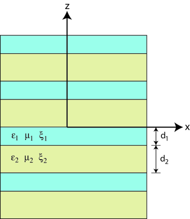
Figure 1: Schematic of the periodic multilayered stack of interest.

Let the $z$ axis of a Cartesian coordinate system be oriented normal to the layers. Provided that both layers in the unit cell are electrically thin, the periodic stack can be homogenized as a uniaxial bianisotropic medium (UBM) whose distinguished axis is the $z$ axis [16]. The frequency-domain constitutive relations of the UBM are given as

$$\left.\begin{array}[]{l}{\bf D}={\varepsilon}_{o}\left[\varepsilon_{\perp}\,\underline{\underline{I}}+(\varepsilon_{\parallel}-\varepsilon_{\perp}){\bf u}_{z}{\bf u}_{z}\right]\mbox{ \tiny{${}^{\bullet}$} }{\bf E}\\ \qquad\qquad+ic_{o}^{-1}\left[\xi_{\perp}\,\underline{\underline{I}}+(\xi_{\parallel}-\xi_{\perp}){\bf u}_{z}{\bf u}_{z}\right]\mbox{ \tiny{${}^{\bullet}$} }{\bf H}\\[5.0pt] {\bf B}=\mu_{o}\left[\mu_{\perp}\,\underline{\underline{I}}+(\mu_{\parallel}-\mu_{\perp}){\bf u}_{z}{\bf u}_{z}\right]\mbox{ \tiny{${}^{\bullet}$} }{\bf H}\\ \qquad\qquad-ic_{o}^{-1}\left[\xi_{\perp}\,\underline{\underline{I}}+(\xi_{\parallel}-\xi_{\perp}){\bf u}_{z}{\bf u}_{z}\right]\mbox{ \tiny{${}^{\bullet}$} }{\bf E}\end{array}\right\}\,,$$ (3)

where $\underline{\underline{I}}$ is the identity dyadic, and there are six effective constitutive parameters: $\varepsilon_{\parallel}$, $\varepsilon_{\perp}$, $\mu_{\parallel}$, $\mu_{\perp}$, $\xi_{\parallel}$, and $\xi_{\perp}$. In the following subsections, we provide two different ways to determine these six scalars in terms of the constitutive parameters and the volume fractions of the two constituent materials in the unit cell.

2.1 4$\times$4-Matrix method

Without loss of generality, wave propagation in the multilayered stack can be handled by using the spatial Fourier transform as

$$\left.\begin{array}[]{l}{\bf E}(x,y,z)=\int_{-\infty}^{\infty}\,{\bf e}(z,\kappa)\exp\left(i\kappa x\right)\,d\kappa\\[5.0pt] {\bf H}(x,y,z)=\int_{-\infty}^{\infty}\,{\bf h}(z,\kappa)\exp\left(i\kappa x\right)\,d\kappa\end{array}\right\}\,,$$ (4)

whereby the fields are assumed not to vary along the $y$ axis. The spatial frequency along the $x$ axis is denoted by $\kappa$. Substitution of this representation along with the constitutive relations (1) in the two Maxwell curl equations leads to the 4$\times$4-matrix ordinary differential equation [18]

$$\frac{d}{dz}\left[{\bf F}(z,\kappa)\right]=i\left[\underline{\underline{P}}^{(n)}(\kappa)\right]\mbox{ \tiny{${}^{\bullet}$} }\left[{\bf F}(z,\kappa)\right]$$ (5)

in any layer made of the $n$-th material. Here, the column vector

$$\left[{\bf F}(z,\kappa)\right]=\left[\begin{array}[]{c}e_{x}(z,\kappa)\\ e_{y}(z,\kappa)\\ h_{x}(z,\kappa)\\ h_{y}(z,\kappa)\end{array}\right]$$ (6)

represents components of the electric and magnetic fields that are tangential to the bimaterial interfaces in the multilayered stack, whereas the 4$\times$4 matrix

$$\left[\underline{\underline{P}}^{(n)}(\kappa)\right]=\omega\left[\begin{array}[]{cccc}0&-i\xi_{n}/c_{o}&0&\mu_{o}\mu_{n}\\ i\xi_{n}/c_{o}&0&-\mu_{o}\mu_{n}&0\\ 0&-{\varepsilon}_{o}\varepsilon_{n}&0&-i\xi_{n}/c_{o}\\ {\varepsilon}_{o}\varepsilon_{n}&0&i\xi_{n}/c_{o}&0\end{array}\right]$$ (11)

$$\qquad+\frac{\kappa^{2}}{\omega\left(\varepsilon_{n}\mu_{n}-\xi_{n}^{2}\right)}\,\left[\begin{array}[]{cccc}0&-i\xi_{n}c_{o}&0&-\mu_{n}/{\varepsilon}_{o}\\ 0&0&0&0\\ 0&\varepsilon_{n}/\mu_{o}&0&-i\xi_{n}c_{o}\\ 0&0&0&0\end{array}\right]\,,\quad n=1,2\,,$$ (16)

contains all three constitutive parameters, the angular frequency, and the parameter $\kappa$ denoting propagation along the $x$ axis.

A similar exercise for wave propagation in the homogenized medium (i.e., the equivalent UBM) yields the 4$\times$4-matrix ordinary differential equation [18]

$$\frac{d}{dz}\left[{\bf F}(z,\kappa)\right]=i\left[\underline{\underline{P}}^{eqvt}(\kappa)\right]\mbox{ \tiny{${}^{\bullet}$} }\left[{\bf F}(z,\kappa)\right]\,,$$ (17)

where

$$\left[\underline{\underline{P}}^{eqvt}(\kappa)\right]=\omega\left[\begin{array}[]{cccc}0&-i\xi_{\perp}/c_{o}&0&\mu_{o}\mu_{\perp}\\ i\xi_{\perp}/c_{o}&0&-\mu_{o}\mu_{\perp}&0\\ 0&-{\varepsilon}_{o}\varepsilon_{\perp}&0&-i\xi_{\perp}/c_{o}\\ {\varepsilon}_{o}\varepsilon_{\perp}&0&i\xi_{\perp}/c_{o}&0\end{array}\right]$$ (22)

$$\qquad+\frac{\kappa^{2}}{\omega\left(\varepsilon_{\parallel}\mu_{\parallel}-\xi_{\parallel}^{2}\right)}\,\left[\begin{array}[]{cccc}0&-i\xi_{\parallel}c_{o}&0&-\mu_{\parallel}/{\varepsilon}_{o}\\ 0&0&0&0\\ 0&\varepsilon_{\parallel}/\mu_{o}&0&-i\xi_{\parallel}c_{o}\\ 0&0&0&0\end{array}\right]\,.$$ (27)

As both layers in the unit cell are electrically thin, we can invoke the long-wavelength approximation [19] to set

$$\left[\underline{\underline{P}}^{eqvt}(\kappa)\right]=f_{1}\left[\underline{\underline{P}}^{(1)}(\kappa)\right]+f_{2}\left[\underline{\underline{P}}^{(2)}(\kappa)\right]\,.$$ (28)

With

$$\Delta=(f_{1}\varepsilon_{2}+f_{2}\varepsilon_{1})(f_{1}\mu_{2}+f_{2}\mu_{1})-(f_{1}\xi_{2}+f_{2}\xi_{1})^{2}\,,$$ (29)

this procedure yields the following expressions for the effective constitutive parameters of the stack:

$$\varepsilon_{\perp}=f_{1}\varepsilon_{1}+f_{2}\varepsilon_{2}\,,$$ (30)

$$\varepsilon_{\parallel}=\Delta^{-1}\left[{f_{1}\varepsilon_{1}(\varepsilon_{2}\mu_{2}-\xi_{2}^{2})+f_{2}\varepsilon_{2}(\varepsilon_{1}\mu_{1}-\xi_{1}^{2})}\right]\,,$$ (31)

$$\mu_{\perp}=f_{1}\mu_{1}+f_{2}\mu_{2}\,,$$ (32)

$$\mu_{\parallel}=\Delta^{-1}\left[{f_{1}\mu_{1}(\varepsilon_{2}\mu_{2}-\xi_{2}^{2})+f_{2}\mu_{2}(\varepsilon_{1}\mu_{1}-\xi_{1}^{2})}\right]\,,$$ (33)

$$\xi_{\perp}=f_{1}\xi_{1}+f_{2}\xi_{2}\,,$$ (34)

$$\xi_{\parallel}=\Delta^{-1}\left[{f_{1}\xi_{1}(\varepsilon_{2}\mu_{2}-\xi_{2}^{2})+f_{2}\xi_{2}(\varepsilon_{1}\mu_{1}-\xi_{1}^{2})}\right]\,.$$ (35)

Thus, whereas the mixing of the constitutive parameters of the two layers of the unit cell is trivially simple in the transversely isotropic components ($\varepsilon_{\perp}$, $\mu_{\perp}$, $\xi_{\perp}$) of the constitutive dyadics of the equivalent UBM, the mixing is far richer in the axial components ($\varepsilon_{\parallel}$, $\mu_{\parallel}$, $\xi_{\parallel}$) of those dyadics. Our focus is on these axial components.

2.2 Method of boundary conditions

A critical question that arises in any homogenization procedure is, whether the procedure preserves the boundary conditions across interfaces that are imposed by the Maxwell equations on the electromagnetic fields. In this subsection, we obtain the effective constitutive dyadics of the periodic multilayered stack by considering the boundary conditions on the electromagnetic fields. The obtained parameters are identical to the ones obtained by the procedure of Sec. 2.1, which is a matter of consistency.

In the limit of very small layer thickness (compared to the wavelength of light), the electromagnetic fields can be assumed to be reasonably uniform across a unit cell of the periodic stack. But they have to satisfy the appropriate boundary conditions across the bimaterial interfaces. Suppose the fields in layer $n$, $n\in\left[1,2\right]$, of the unit cell are denoted by ${\bf E}_{n}$, ${\bf H}_{n}$, ${\bf D}_{n}$, and ${\bf B}_{n}$. Let us first consider the continuity of the tangential components (i.e., oriented parallel to the $xy$ plane) of the $\mathbf{E}$ and $\mathbf{H}$ fields:

$$\mathbf{E}_{1tan} =\mathbf{E}_{2tan} =\langle\mathbf{E}_{tan}\rangle,$$ (36)

$$\mathbf{H}_{1tan} =\mathbf{H}_{2tan} =\langle\mathbf{H}_{tan}\rangle,$$ (37)

where $\langle\mathbf{E}_{tan}\rangle$ and $\langle\mathbf{H}_{tan}\rangle$ are the volume-averaged fields. Now considering the volume-averaged fields $\langle\mathbf{D}_{tan}\rangle$ and $\langle\mathbf{B}_{tan}\rangle$ defined as

$$\langle\mathbf{D}_{tan}\rangle =f_{1}\mathbf{D}_{1{tan}}+f_{2}\mathbf{D}_{2{tan}} =\varepsilon_{0}\varepsilon_{\perp}\langle\mathbf{E}_{tan}\rangle+ic_{o}^{-1}\xi_{\perp}\langle\mathbf{H}_{tan}\rangle,$$ (38)

$$\langle\mathbf{B}_{tan}\rangle =f_{1}\mathbf{B}_{1{tan}}+f_{2}\mathbf{B}_{2{tan}} =\mu_{0}\mu_{\perp}\langle\mathbf{H}_{tan}\rangle-ic_{o}^{-1}\xi_{\perp}\langle\mathbf{E}_{tan}\rangle,$$ (39)

we obtain

$$\varepsilon_{\perp} = f_{1}\varepsilon_{1}+f_{2}\varepsilon_{2},$$ (40)

$$\mu_{\perp} = f_{1}\mu_{1}+f_{2}\mu_{2},$$ (41)

$$\xi_{\perp} = f_{1}\xi_{1}+f_{2}\xi_{2}$$ (42)

for the equivalent UBM. These results are identical to those given by Eqs. (30), (32), and (34), respectively.

Next, let us consider the continuity of the electromagnetic field components normal to the bimaterial interfaces (i.e., oriented along the $z$ axis) as follows:

$$\langle\mathbf{D}_{norm}\rangle=\mathbf{D}_{1{norm}}=\mathbf{D}_{2{norm}},$$ (43)

$$\langle\mathbf{B}_{norm}\rangle=\mathbf{B}_{1{norm}}=\mathbf{B}_{2{norm}},$$ (44)

$$\langle\mathbf{E}_{norm}\rangle=f_{1}\mathbf{E}_{1{norm}}+f_{2}\mathbf{E}_{2{norm}},$$ (45)

$$\langle\mathbf{H}_{norm}\rangle=f_{1}\mathbf{H}_{1{norm}}+f_{2}\mathbf{H}_{2{norm}}.$$ (46)

Using the constitutive relations (3) of the homogenized material, we obtain the following three relations from the foregoing equations:

$$\frac{\varepsilon_{\parallel}}{\varepsilon_{\parallel}\mu_{\parallel}-\xi_{\parallel}^{2}} = f_{1}\frac{\varepsilon_{1}}{\varepsilon_{1}\mu_{1}-\xi_{1}^{2}}+f_{2}\frac{\varepsilon_{2}}{\varepsilon_{2}\mu_{2}-\xi_{2}^{2}}\,,$$ (47)

$$\frac{\mu_{\parallel}}{\varepsilon_{\parallel}\mu_{\parallel}-\xi_{\parallel}^{2}} = f_{1}\frac{\mu_{1}}{\varepsilon_{1}\mu_{1}-\xi_{1}^{2}}+f_{2}\frac{\mu_{2}}{\varepsilon_{2}\mu_{2}-\xi_{2}^{2}}\,,$$ (48)

$$\frac{\xi_{\parallel}}{\varepsilon_{\parallel}\mu_{\parallel}-\xi_{\parallel}^{2}} = f_{1}\frac{\xi_{1}}{\varepsilon_{1}\mu_{1}-\xi_{1}^{2}}+f_{2}\frac{\xi_{2}}{\varepsilon_{2}\mu_{2}-\xi_{2}^{2}}\,.$$ (49)

The solutions of these three equations are given by Eqs. (31), (33), and (35). Let us reiterate that, as all expressions derived in this section involve only the volume fractions and not the individual layer thicknesses, they are valid only in the limit of small layer thicknesses.

The quantities $\varepsilon_{\parallel}$, $\mu_{\parallel}$, and $\xi_{\parallel}$ satisfy the relation

$${\rm Det}\left[\begin{array}[]{ccc}\varepsilon_{1}&\varepsilon_{2}&\varepsilon_{\parallel}\\[5.0pt] \mu_{1}&\mu_{2}&\mu_{\parallel}\\[5.0pt] \xi_{1}&\xi_{2}&\xi_{\parallel}\end{array}\right]=0\,.$$ (50)

This relation implies that both homogenization procedures yield only two of the three quantities $\varepsilon_{\parallel}$, $\mu_{\parallel}$, and $\xi_{\parallel}$ independently; the third can be obtained from Eq. (50). This feature of homogenization has been remarked upon earlier for dispersions of electrically small, isotropic chiral spheres in an isotropic achiral host material [20].

3 Numerical Results and Discussion

In order to prove the premise of this paper, let us set material $1$ to be achiral, i.e., $\xi_{1}=0$. Furthermore, without loss of generality, let both materials $1$ and $2$ be nonmagnetic in the Tellegen representation: $\mu_{1}=\mu_{2}=1$. In that case, $\mu_{\perp}=1$ whereas

$$\mu_{\parallel}=\frac{(f_{1}\varepsilon_{2}+f_{2}\varepsilon_{1})-f_{1}\xi_{2}^{2}}{(f_{1}\varepsilon_{2}+f_{2}\varepsilon_{1})-f_{1}^{2}\xi_{2}^{2}}\,.$$ (51)

Now, we can explore the effect of $\xi_{2}$ on the sign of ${\rm Re}\left(\varepsilon_{\parallel}\right)$.

Suppose further that material $1$ is silver, so that [21]

$$\varepsilon_{1}(\lambda_{o})=5.7+0.4i-\left(\frac{9q}{2\pi c_{o}\hbar}\right)^{2}\lambda_{o}^{2}\,.$$ (52)

where $q=1.6022\times 10^{-19}$ C is the charge of an electron and $\hbar=1.0546\times 10^{-34}$ J s is the reduced Planck constant. This expression is valid for $\lambda_{o}\in\left[300,900\right]$ nm. It has been used, for example, by Pendry [22] and also fits the data of Stahrenberg et al. [23] in the chosen spectral regime. For $\varepsilon_{2}$, we choose the Lorentz model

$$\varepsilon_{2}(\lambda_{o})=2+\frac{C_{2}}{1-\left(\frac{\lambda_{2}}{\lambda_{o}}\right)^{2}-\frac{i\gamma_{2}\lambda_{2}}{2\pi c_{o}}\,\left(\frac{\lambda_{2}}{\lambda_{o}}\right)}\,,$$ (53)

wherein $C_{2}$, $\lambda_{2}$, and $\gamma_{2}$ are constants. The values of these parameters chosen for the following studies are typical of solid materials; in addition, they keep the magnitudes of $\varepsilon_{2}$ from becoming unphysically large in the resonance regime.

Figure 2 contains plots of $\varepsilon_{\parallel}$ and $\xi_{\parallel}$ with respect to free-space wavelength, when material $2$ is nondispersive and nondissipative, and $\xi_{2}=0.05$. The resonant frequency evident in these plots is due to the condition $\Delta=0$; hence, it is fixed by the volume fraction of silver ($f_{1}=0.58$ for this figure) and is affected by the dispersive properties of silver. The width of the resonance is proportional to the volume fraction of the dissipative material (i.e., silver). For physically realistic values of $\xi_{2}$ ($\lesssim 10^{-3}$), the resonance condition $\Delta=0$ can be achieved only if the ratio ${\rm Re}(\varepsilon_{2})/{\rm Re}(\varepsilon_{1})<0$.

The resonance condition enhances $\xi_{\parallel}$. This becomes clear by noting that the maximum value of $|\xi_{\parallel}|$ is many times larger than that of the chirality parameter $\xi_{2}$ of the isotropic chiral constituent of the multilayered stack. In contrast, Eq. (34) indicates that $\xi_{\perp}$ is diluted in relation to $\xi_{2}$ by the volume fraction of material $2$.

The resonance condition also enhances ${\rm Im}(\varepsilon_{\parallel})$ far above the imaginary part of the relative permittivity of silver. This is deleterious to wave propagation inside the multilayered stack. Still, we cannot help remarking that frequency regimes exist (e.g., $\lambda_{o}\approx 500$ nm) wherein $\xi_{\parallel}$ is significantly enhanced whereas ${\rm Im}(\varepsilon_{\parallel})$ is significantly reduced in relation to ${\rm Im}(\varepsilon_{1})$.

Let us also note that the homogenized medium, a UBM, has the properties of a chiroplasma except for a gyrotropic term, because such a term is missing in both constituent materials [24]. It also presents an example of a homogeneous medium that displays chirality along with a negative real permittivity at optical frequencies, which has not been reported earlier, to our knowledge.

Figure 3 presents a highly magnified view of $\varepsilon_{\parallel}$ in the resonance region ($\lambda_{o}\approx 400$ nm). The constitutive properties and geometric parameters are the same as in the previous figure, except that data is shown for both $\xi_{2}=0$ and $\xi_{2}=0.05$. Clearly, the zero-crossing of ${\rm Re}(\varepsilon_{\parallel})$ blueshifts by about $0.5$ Å, when $\xi_{2}$ increases from $0$ to $0.05$, furthermore, the same blueshift would occur even if $\xi_{2}$ were to be replaced by $-\xi_{2}$. This spectroscopic shift is measurable [15].

We have not shown spectral plots of $\mu_{\parallel}$, because its magnitude is very close to unity. It does, however, evince a resonance, just like $\varepsilon_{\parallel}$ and $\xi_{\parallel}$ and at the same frequency.

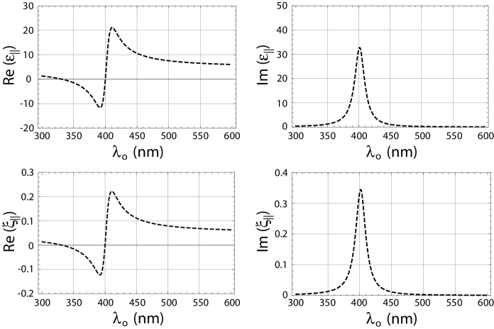
Figure 2: Real and imaginary parts of $\varepsilon_{\parallel}$, and real and imaginary parts of $\xi_{\parallel}$, as functions of free-space wavelength, when $f_{1}=0.58$, $C_{2}=0$, and $\xi_{2}=0.05$.

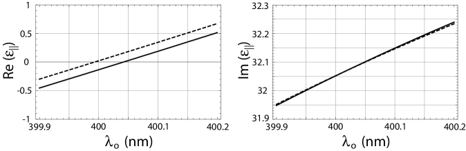
Figure 3: Real and imaginary parts of $\varepsilon_{\parallel}$ as functions of free-space wavelength, when $f_{1}=0.58$ and $C_{2}=0$; $\xi_{2}=0$ (solid lines) and $\xi_{2}=0.05$ (dashed lines).

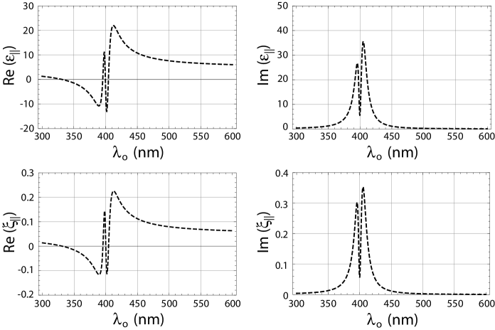
Figure 4: Real and imaginary parts of $\varepsilon_{\parallel}$, and real and imaginary parts of $\xi_{\parallel}$, as functions of free-space wavelength, when $f_{1}=0.58$, $C_{2}=10^{-3}$, $\lambda_{2}=400$ nm, $\gamma_{2}=10^{13}$ rad s^-1, and $\xi_{2}=0.05$.

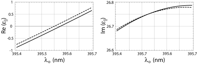
Figure 5: Real and imaginary parts of $\varepsilon_{\parallel}$ as functions of free-space wavelength, when $f_{1}=0.58$, $C_{2}=10^{-3}$, $\lambda_{2}=400$ nm, and $\gamma_{2}=10^{13}$ rad s^-1; $\xi_{2}=0$ (solid lines) and $\xi_{2}=0.05$ (dashed lines).

Let us now move on to the situation where the relative permittivity of material $2$ is both dissipative and dispersive. In order to investigate the interplay of structural resonance (evident in Fig. 2) and intrinsic material resonance, we set $\lambda_{2}=400$ nm; furthermore, $C_{2}=10^{-3}$ and $\gamma_{2}=10^{13}$ rad s^-1. Figure 4 clearly shows the doubly-resonant characteristics of $\varepsilon_{\parallel}$ and $\xi_{\parallel}$, arising from this interplay. Chirality enhancement is again evident in this figure, as also the enhancement of ${\rm Im}(\varepsilon_{\parallel})$.

The double resonance in the spectra implies that there are three zero-crossings of ${\rm Re}(\varepsilon_{\parallel})$. Figure 5 presents a highly magnified view of $\varepsilon_{\parallel}$ near one of the three zero-crossings for both $\xi_{2}=0$ and $\xi_{2}=0.05$. A blueshift of $0.25$ Å is evident, which, we reiterate, is measurable [15].

We also calculated the linear remittances (i.e., the reflectances and transmittances) of a 20-period multilayered stack that was about a wavelength thick. The presence of isotropic chirality resulted in the aforementioned blueshifts in the effective constitutive parameters of the stack, and manifested as small changes in the remittances at oblique incidence. Cross-polarized remittances on the order of 1% were seen when $\xi_{2}\neq 0$, but were of course absent for $\xi_{2}=0$. At normal incidence, $\xi_{2}$ played no role at all, which becomes clear from setting $\kappa=0$ on the right side of Eq. (27); instead, the stack behaves as a dilute metal.

Our focus on spectroscopic shifts at the boundary of the visible and the ultraviolet regimes is in accord with the fact that the chirality of many isotropic materials is evident in both regimes. Examples include suspensions of poly-L-glutamic acid [25], solutions of glucose [26] and several derivatives of cellulose [27], and chiral barbituric acid [28]. Flooding a multilayered stack containing void regions alternating with metallic layers with isotropic chiral fluids is a way to dynamically blueshift the zero-crossing of ${\rm Re}\left(\varepsilon_{\parallel}\right)$.

Let us note that we have used $\xi_{2}=0.05$ in order to illustrate the spectral shifts due to chirality. Chirality paramaters of natural as well as synthetic materials available in the published literature are smaller. However, values of $|\xi_{2}|\sim 0.1$ at microwave frequencies have recently been obtained [14]. When such large chirality parameters would become available at optical frequencies, even larger spectral shifts would be possible. Effectively, the shift of the resonance frequency can enable the use of such stacks as tunable high-pass filters for spectroscopy. The use of two such filters in tandem can enable a narrow-bandwidth source at almost any desired frequency. Dissipation is, however, a cause for deep concern. We are investigating the possibility of making infrared filters using layers of low-dissipation polaritonic crystals with negative real permittivity (such as LiTaO₃ resonance at about 26.7 THz or silicon carbide in the mid-infrared regime) and isotropic chiral materials. Such filters could be effectively used for spectroscopy of molecular vibro-rotational levels.

4 Concluding Remarks

To conclude, we derived the effective constitutive parameters of a period multilayered stack whose unit cell comprises a metallic layer and an isotropic chiral layer. We found that the stack behaves as an anisotropic metamaterial with resonant response that is determined primarily by the volume fraction of the metal. The presence of isotropic chirality can result in small shifts of the resonance frequency for reasonably large values of the chirality parameter; hence, the sign of one of the two effective permittivities of the stack can be switched. The spectral shifts in the dielectric properties can be potentially useful for spectroscopic purposes.

References

References

- [1] Ramakrishna S A 2005 Rept. Prog. Phys. 68 449
- [2] Wood B 2007 Laser Photon. Rev. 1 249
- [3] O’Brien S, McPeake D, Ramakrishna S A and Pendry J B 2004 Phys. Rev. B 69 241101
- [4] Chen H-T, O’Hara J F, Azad A K., Taylor A J, Averitt R D, Shrekenhamer D B and Padilla W J 2008 Nature Photon. 2 295
- [5] Lakhtakia A 1990 Selected Papers on Natural Optical Activity (Bellingham, WA, USA: SPIE)
- [6] Lakhtakia A, Varadan V V and Varadan V K 1986 IEEE Trans. Electromag. Compat. 28 90
- [7] Tretyakov S, Nefedov I, Sihvola A, Maslovski S and Simovski C 2003 J. Electromag. Waves Appl. 17 695
- [8] Pendry J B 2004 Science 306 1353
- [9] Mackay T G and Lakhtakia A 2004 Phys. Rev. E 69 026602
- [10] Mackay T G 2005 Microw. Opt. Technol. Lett. 45 120; corrections: 2006 47 406
- [11] Bohren C F 2003 in: Weiglhofer W S and Lakhtakia A 2003 Introduction to Complex Mediums for Optics and Electromagnetics (Bellingham, WA, USA: SPIE)
- [12] Varadan V V, Ro R and Varadan V K 1994 Radio Sci. 29 9
- [13] Chung C Y and Whites K W 1996 J. Electromag. Waves Appl. 10 1363
- [14] Gómez A, Lakhtakia A, Margineda J, Molina-Cuberos G J, Núñez J, Ipiña J S, Vegas A and Solano M A 2008 IEEE Trans. Microw. Theory Tech. (accepted for publication)
- [15] http://www.oceanoptics.com/Products/hr4000.asp (24 July 2008)
- [16] Weiglhofer W S 1994 Int. J. Electron. 77 105
- [17] Chen H C 1992 Theory of Electromagnetic Waves (Fairfax, VA, USA: TechBooks)
- [18] Lakhtakia A 1992 Optik 90 184
- [19] Lakhtakia A and Krowne C M 2003 Optik 114 305
- [20] Lakhtakia A, Varadan V K and Varadan V V 1992 J. Mater. Res. 8 917
- [21] Hao F and Nordlander P 2007 Chem. Phys. Lett. 446 115
- [22] Pendry J B 2000 Phys. Rev. Lett. 85 3966
- [23] Stahrenberg K, Herrmann Th, Wilmers K, Esser N, Richter W and Lee M J G 2001 Phys. Rev. B 64 115111
- [24] Weiglhofer W S and Lakhtakia A 1998 Microw. Opt. Technol. Lett. 17 405
- [25] Urry D W and Krivacic J 1970 Proc. Nat. Acad. Sci. USA 65 845
- [26] Lin J-Y, Chen K-H and Su D-C 2004 Opt. Commun. 238 113
- [27] Rakhmanberdyev G R, Fedyakova N A, Myagkova N V and Sidikov A 1996 Chem. Natural Comp. 32 734
- [28] Yeh C and Richardson F S 1975 Theor. Chim. Acta 39 197