A downturn in intergalactic C iv as redshift 6 is approached

Abstract

We present the results of the largest survey to date for intergalactic metals at redshifts $z>5$, using near-IR spectra of nine QSOs with emission redshifts $z_{\rm em}>5.7$. We detect three strong C iv doublets at $z_{\rm abs}=5.7$–5.8, two low ionisation systems at $z_{\rm abs}>5$, and numerous Mg ii absorbers at $z_{\rm abs}=2.5$–2.8. We find, for the first time, a change in the comoving mass density of C iv ions as we look back to redshifts $z>5$. At a mean $\langle z\rangle=5.76$, we deduce $\Omega_{\rm C\,\textsc{iv}}=(4.4\pm 2.6)\times 10^{-9}$ which implies a drop by a factor of $\sim 3.5$ compared to the value at $z<4.7$, after accounting for the differing sensitivities of different surveys. The observed number of C iv doublets is also lower by a similar factor, compared to expectations for a non-evolving column density distribution of absorbers.

These results point to a rapid build-up of intergalactic C iv over a period of only $\sim 300$ Myr; such a build-up could reflect the accumulation of metals associated with the rising levels of star formation activity from $z\sim 9$ indicated by galaxy counts, and/or an increasing degree of ionisation of the intergalactic medium (IGM), following the overlap of ionisation fronts from star-forming regions. If the value of $\Omega_{\rm C\,\textsc{iv}}$ we derive is typical of the IGM at large, it would imply a metallicity $Z_{\rm IGM}\lower 2.15277pt\hbox{$\;\buildrel>\over{\sim}\;$}10^{-4}\,Z_{\odot}$. The early-type stars responsible for synthesising these metals would have emitted only about one Lyman continuum photon per baryon prior to $z=5.8$; such a background is insufficient to keep the IGM ionised and we speculate on possible factors which could make up the required shortfall.

1 Introduction

It is quite remarkable that elements heavier than helium exist in the intergalactic medium (IGM) only $\sim 1$ Gyr after the Big Bang, as indicated by the presence of metal absorption lines associated with the Ly$\alpha$ forest of high redshift QSOs (Songaila 2001; Becker et al. 2006; Ryan-Weber, Pettini & Madau 2006; Simcoe 2006). For these elements to be observed there needs to be significant star formation prior to redshift $z=6$, and the nucleosynthetic products of such early stars need to be expelled beyond the gravitational influence of their host galaxies. The production of early metals is closely linked to the emission of the Lyman continuum (LyC) photons responsible for ionizing the IGM and ending the so-called “dark ages” (Gnedin & Ostriker 1997; Fan, Carilli, & Keating 2006), a process which could have started as early as $z=20$ and continued until completion at $z\sim 6$ (Dunkley et al. 2009).

Clearly, some galaxies were already actively forming stars at $z>6$. The current record for a spectroscopically confirmed galaxy is held by the Ly$\alpha$ emitter at $z=6.96$ discovered by Iye et al. (2006), but several candidates selected via the redshifted Lyman break have been found at $z>7$ (Stark et al. 2007; Richard et al. 2008; Bouwens et al. 2008 and references therein). Furthermore, analyses of the broad-band spectra of galaxies at redshifts $z=2-6$ have in several cases revealed objects with ‘mature’ stellar populations, suggesting that star formation in these galaxies was underway well before $z=6$ (Shapley et al. 2001; Shapley et al. 2005; Yan et al. 2006; Eyles et al. 2007).

Whether the level of star formation so far accounted for at $z>6$ is in fact sufficient to maintain reionization is far less certain, because it depends on a number of essentially unknown parameters, especially the escape fraction of Lyman continuum photons from the sites of star formation, the degree of clumping of the sources and of the IGM, and the slope of the faint end of the galaxy luminosity function at these early times (Madau, Haardt, & Rees 1999). Using the luminosity function of Bouwens et al. (2006) at $z\simeq 6$ and assuming an escape fraction of 20%, Bolton & Haehnelt (2007) concluded that there may be just enough LyC photons to keep the IGM ionised, suggesting that cosmic reionization was a ‘photon starved’ process (see also Gnedin 2008). QSOs are unlikely to help matters, since their contribution to the metagalactic photoionization rate at these redshifts is estimated to be at most 15% (Srbinovsky & Wyithe 2007). Bolton & Haehnelt (2007) proposed that, in order to complete reionization by $z\simeq 6$, either the escape fraction of LyC photons must have been higher at earlier times, or the ionizing spectrum must have been harder (or both). Alternatively, the faint end slope of the luminosity function may have been steeper at $z>6$ compared to the luminosity function determined by Bouwens et al. (2006), as indeed proposed by Stark et al. (2007).

The cosmic budget of elements produced via stellar nucleosynthesis (loosely referred to as metals) provides an entirely different, and complementary, census of the star-formation activity prior to a given epoch. Indeed, at redshifts $z=2-3$ there appears to be an approximate agreement (within a factor of about two) between the observed metal budget—summing together the contributions of stars, IGM and diffuse gas in galaxies—and expectations based on the integral of the cosmic star formation rate density over the first 2-3 Gyr of the Universe history (Pettini 2006; Bouché et al. 2007).

At higher redshifts, we rely increasingly on the Ly$\alpha$ forest and gamma-ray burst afterglows to trace metals in the IGM and in galaxies, since at $z>5$ the spectra of even the most luminous galaxies are too faint to be studied in detail with current instrumentation. The most commonly encountered metal lines associated with the Ly$\alpha$ forest are the C iv $\lambda\lambda 1548.2041,1550.7812$ doublet (Cowie et al. 1995; Ellison et al. 2000). Photoionisation modelling (Schaye et al. 2003; Simcoe, Sargent, & Rauch 2004) suggests that at redshifts $z=2-3$ the carbon abundance is a function of the gas density, as expected (Cen & Ostriker 1999), and that the mean metallicity of the IGM is $Z_{\rm IGM}\approx 1/1000\,Z_{\odot}$.

Interestingly, the comoving mass density of triply ionised carbon, obtained by integrating the distribution of column densities $N$(C iv), appears to be approximately constant from $z\simeq 5$ to $z\simeq 1.5$: expressed as a fraction of the critical density, $\Omega_{\rm C\,\textsc{iv}}\simeq(1-4)\times 10^{-8}$ (Songaila 2001; Pettini et al. 2003) over a period of $\sim 3$ Gyr which saw the peak of the cosmic star-formation and massive black hole activity (e.g. Reddy et al. 2008 and references therein). This surprising result has led to conflicting interpretations as to the source of these intergalactic metals, with some authors (e.g. Madau, Ferrara, & Rees 2001; Porciani & Madau 2005) proposing an origin in low-mass galaxies at $z\gg 6$, when the pollution of large volumes of the IGM would have been easier, while others (e.g Adelberger 2005) place them much closer to the massive galaxies responsible for most of the metal production at redshifts $z=1.5$–5. While both processes presumably contribute, their relative importance has yet to be established with certainty (Songaila 2006).

The most extensive theoretical work in this area has been published by B. D.  Oppenheimer and collaborators. In a series of papers (Oppenheimer & Davé 2006, 2008; Davé & Oppenheimer 2007) these authors analysed the output of cosmological simulations of galaxy formation which include feedback in the form of momentum-driven winds. They found that the apparent lack of evolution of $\Omega_{\rm C\,\textsc{iv}}$ from $z=5$ to 1.5 can be explained as the result of two countervailing effects: an overall increase of the cosmic abundance of carbon, reflecting the on-going pace of star formation, and an accompanying reduction in the fraction of carbon which is triply ionised.

Whether this is the true picture or not, it is clear that determining $\Omega_{\rm C\,\textsc{iv}}$ at $z>5$ is the next observational priority; in any case, metal lines are our only remaining probe of the IGM at these high redshifts where the Ly$\alpha$ forest itself becomes effectively opaque. Such an extension of metal-line surveys in QSO spectra necessitates observations at moderate spectral resolution and signal-to-noise ratio at near-infrared (near-IR) wavelengths, a regime which has only recently begun to be exploited for such purposes (e.g. Kobayashi et al. 2002; Nissen et al. 2007). In a pilot study (Ryan-Weber, Pettini, & Madau 2006), we demonstrated that QSO absorption line spectroscopy could indeed be performed in the near-IR to the levels required to detect intergalactic C iv absorption. From observations of two QSO at redshifts $z_{\rm em}=6.28$ and 5.99 we discovered two strong C iv doublets at absorption redshifts $z_{\rm abs}=5.7238$ and 5.8290. These two absorbers, which were confirmed by an independent study by Simcoe (2006), would—if typical— imply that a high concentration of C iv was already in place in the IGM at $z\simeq 6$, but clearly much better statistics than those afforded by only two QSO sight-lines are necessary to assess the true level of $\Omega_{\rm C\,\textsc{iv}}$.

Given the success of our pilot study, in the last two years we have conducted an observational campaign on the Keck and ESO-VLT telescopes aimed at securing near-IR spectra of as many as possible of the 19 known QSOs with $z_{\rm em}>5.7$ and infrared magnitude $J<19.2$. The results of this programme are presented here. Specifically, we have observed 13 QSOs and obtained useful data for ten of them. This sample represents an increase by a factor of seven in the pathlength probed, from the absorption distance $\Delta X=3.6$ covered by Ryan-Weber et al. (2006) to $\Delta X=25.1$. With this extended data set, we find the first evidence for a decrease in $\Omega_{\rm C\,\textsc{iv}}$ from $z\sim 4.7$ to $z\sim 5.8$, in broad agreement with the predictions of the cosmological simulations by Oppenheimer, Davé, & Finlator (2009).

This paper is organised as follows. Section 2 describes the observations, followed by brief comments on each QSO in Section 3. In Section 4 we deduce the value of $\Omega_{\rm C\,\textsc{iv}}$ implied from our three detections of C iv absorbers within the redshift range $5.2\leq z_{\rm abs}\leq 6.2$. In Sections 5 and 6, we consider the completeness of the survey, and discuss the evidence for a drop in $\Omega_{\rm C\,\textsc{iv}}$ as we look back to redshifts $z>4.7$. The implications of these results for early star formation and reionisation are discussed in Section 7. We finally summarise our main conclusions in Section 8.

Throughout this paper we use a ‘737’ cosmology with $H_{0}=70$ km s^-1 Mpc^-1, $\Omega_{\rm M}=0.3$ and $\Omega_{\Lambda}=0.7$. Much of the previous work (including our own) with which we compare the present results was based on an Einstein-de Sitter cosmology; in all cases, we have converted the quantities of interest to the cosmology adopted here.

Table 1: Details of the Observations

QSO	$J_{\rm Vega}$	$z_{\rm em}$	Telescope/	Wavelength	Resolution	Integration	S/Na	$\Delta z^{\rm b}$
	(mag)		Instrument	Range (Å)	(km s-1)	Time (s)
ULAS J020332.38+001229.2	19.1	5.706c	Keck ii/NIRSPEC	10 219–10 588	185	6 300	10–13	5.601–5.639d
SDSS J081827.40+172251.8	18.5	6.00	VLT1/ISAAC	9 877–10 790e	53	32 400f	8–13	5.380–5.930e
SDSS J083643.85+005453.3	17.9	5.810g	VLT1/ISAAC	10 100–10 550	53	16 200	8	5.524–5.752
SDSS J084035.09+562419.9	19.0	5.774c	Keck ii/NIRSPEC	9 548–11 140	185	11 700	10–22	5.167–5.706
SDSS J103027.01+052455.0h	18.9	6.309i	VLT1/ISAAC	9 880–10 780e	53	82 800j	5–7	5.382–5.951e
SDSS J113717.73+354956.9	18.4	5.962c	Keck ii/NIRSPEC	9 542–11 172	185	9 000	20–40	5.163–5.893
SDSS J114816.64+525150.2	18.1	6.421k	Keck ii/NIRSPEC	9 572–11 159	185	18 000	16–30	5.183–6.196
SDSS J130608.26+035626.3h	18.8	6.016i	VLT1/ISAAC	9 914–10 332	53	7 200	5	5.404–5.662
SDSS J160253.98+422824.9	18.5	6.051c	Keck ii/NIRSPEC	9 553–11 143	185	9 900	17–48	5.170–5.981
SDSS J205406.49$-$000514.8	19.2	6.062	Keck ii/NIRSPEC	9 681–10 927	185	5 400	8–12	5.253–5.991

^aSignal-to-noise ratio over wavelength range sampled.

^bRedshift range covered for C iv absorption.

^cWhen available, we quote values of $z_{\rm em}$ measured from the C iv $\lambda 1549.062$ broad emission line in our NIRSPEC spectra. As is well known,

the QSO systemic redshift, $z_{\rm sys}$, can be higher than the value measured from high ionisation lines such as C iv, by up to several thousand km s^-1

(e.g. Richards et al. 2002).

^dBAL QSO; not included in the survey statistics.

^eWith a small gap between two wavelength settings.

^fTwo wavelength settings, with exposure times of 14 400 and 18 000 s respectively.

^gKurk et al. (2007).

^hObservations reported in Ryan-Weber et al. (2006).

ⁱJiang et al. (2007).

^jIn three, partially overlapping, wavelength settings, with exposure times of 39 600, 7 200 and 36 000 s respectively.

^k$z_{\rm em}$ measured from the Si iv $\lambda 1396.752$ broad emission line in our NIRSPEC spectrum.

2 Observations and data reduction

A trawl of the relevant literature reveals that 19 QSOs are currently known with emission redshift $z_{\rm em}>5.7$ and $J$ magnitude brighter than $J\simeq 19.2$. This magnitude is at the faint limit for recording medium-resolution near-IR spectra of S/N $\lower 2.15277pt\hbox{$\;\buildrel>\over{\sim}\;$}5$ with integration times of a few hours on 8-10 m class telescopes using available instrumentation. The redshift cut is required to give a useful pathlength over which to search for C iv absorption at redshifts $z_{\rm abs}>5$, this being the limit of previous surveys (Songaila 2001; Pettini et al. 2003).

Over the four-year period between 2004 and 2008 we observed 13 of these 19 possible targets with NIRSPEC on the Keck ii telescope (McLean et al. 1998) and with ISAAC on VLT-UT1 (Moorwood et al. 1998). For ten QSOs we secured spectra with S/N $\geq 5$; relevant details are collected in Table 1. In the other three cases, the object was not pursued after initial test exposures, either because the spectrum displayed broad absorption lines (SDSS J104433.04$-$012502.2 at $z_{\rm em}=5.74$ and SDSS J104845.05$+$463718.3, $z_{\rm em}=6.20$), or because the QSO turned out to be fainter than anticipated (SDSS J141111.29$+$121737.4, $z_{\rm em}=5.93$). The values of emission redshift $z_{\rm em}$ listed in Table 1 are those measured from the discovery spectra, unless otherwise noted.

2.1 NIRSPEC Observations

With NIRSPEC we used the NIRSPEC 1$+$thin blocker filter combination to record the wavelength region $\sim 9540$–11 170 Å on the ALADDIN-3 InSb detector which has $1024\times 1024$ 27$\mu$m pixels. With the $42\times 0.57$ arcsec entrance slit, the spectrograph delivers a resolution ${\rm FWHM}=6.4$ Å (185 km s^-1 at 10 355 Å), sampled with 2.1 pixels. Typically, we exposed on an object for 900 s before reading out the detector, moving the target by a few arcseconds along the slit, and starting the subsequent exposure. Total integration times ranged between 5400 and 18 000 s (see column (7) of Table 1). All of the QSO observed were sufficiently bright at near-IR wavelengths to be visible on the slit, thereby facilitating guiding.

     

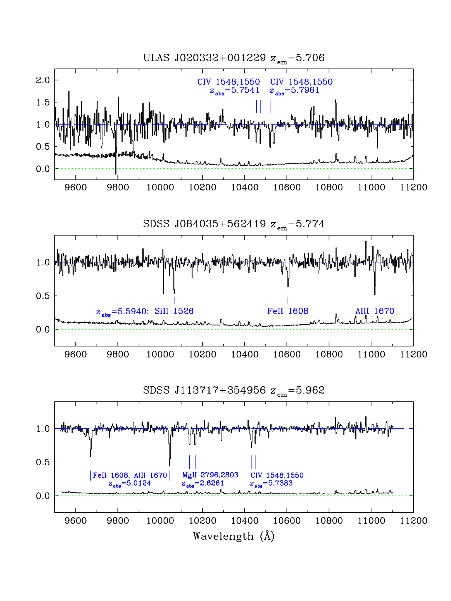
Figure 1: NIRSPEC spectra of ULAS J020332.38+001229.2, SDSS J084035.09+562419.9 and SDSS J113717.73+354956.9. In each panel, the top histogram shows the normalised QSO spectrum, while the lower histogram is the corresponding $1\sigma$ error spectrum. Absorption features are indicated by vertical tick marks and labelled with their identification. The two C iv absorption doublets seen in the spectrum of ULAS J020332.38+001229.2 (top panel) are close to the QSO emission redshift and are probably intrinsic (see section 3.1). Parameters of the C iv doublet identified towards SDSS J113717.73+354956.9 (bottom panel) are listed in Tables 2 and LABEL:tab:abs.

The NIRSPEC two-dimensional (2-D) spectra were processed with a suite of purpose-designed IDL routines kindly provided by Dr. G. Becker. As described in more detail by Becker, Rauch, & Sargent (2009), this software does a very good job at subtracting the dark current, removing detector defects, flat-fielding, and particularly removing the sky background (achieved by employing the optimal sky subtraction techniques of Kelson 2003) which can be the limiting factor to the S/N achievable at near-IR wavelengths. Optimal extraction (Horne 1986) is also used to trace the QSO signal in the processed 2-D images and output a vacuum-heliocentric wavelength calibrated one-dimensional (1-D) source spectrum and associated error. The wavelength calibration uses the OH sky emission lines superposed on the QSO spectrum, with the wavelengths tabulated in the atlas by Rousselot et al. (2000).

As we have many ($\geq 6$) individual 900 s spectra (and associated error) of each of our QSOs, we combined them using a weighted mean algorithm that operates on a pixel-by-pixel basis and rejects outliers beyond a specified number of standard deviations from the mean (usually $\geq 3\sigma$). The spectra were finally normalised by dividing by a spline fit to the underlying QSO continuum. The rms deviation of the data from this continuum (away from obvious spectral features) provides an empirical estimate of the final S/N achieved. We found this empirical estimate of the S/N to be lower, by factors between 2.0 and 1.1, than the pixel-to-pixel error on the weighted mean calculated when co-adding the individual exposures, as described above. This difference presumably reflects the residual importance of systematic (rather than random) errors; in any case, the values listed in the penultimate column of Table 1 are those measured from the residuals about the continuum fit. Since the S/N varies along each spectrum, we give in the Table the maximum and minimum values which apply to the wavelength region searched for absorption lines (listed for each QSO in column (5) of Table 1).

     

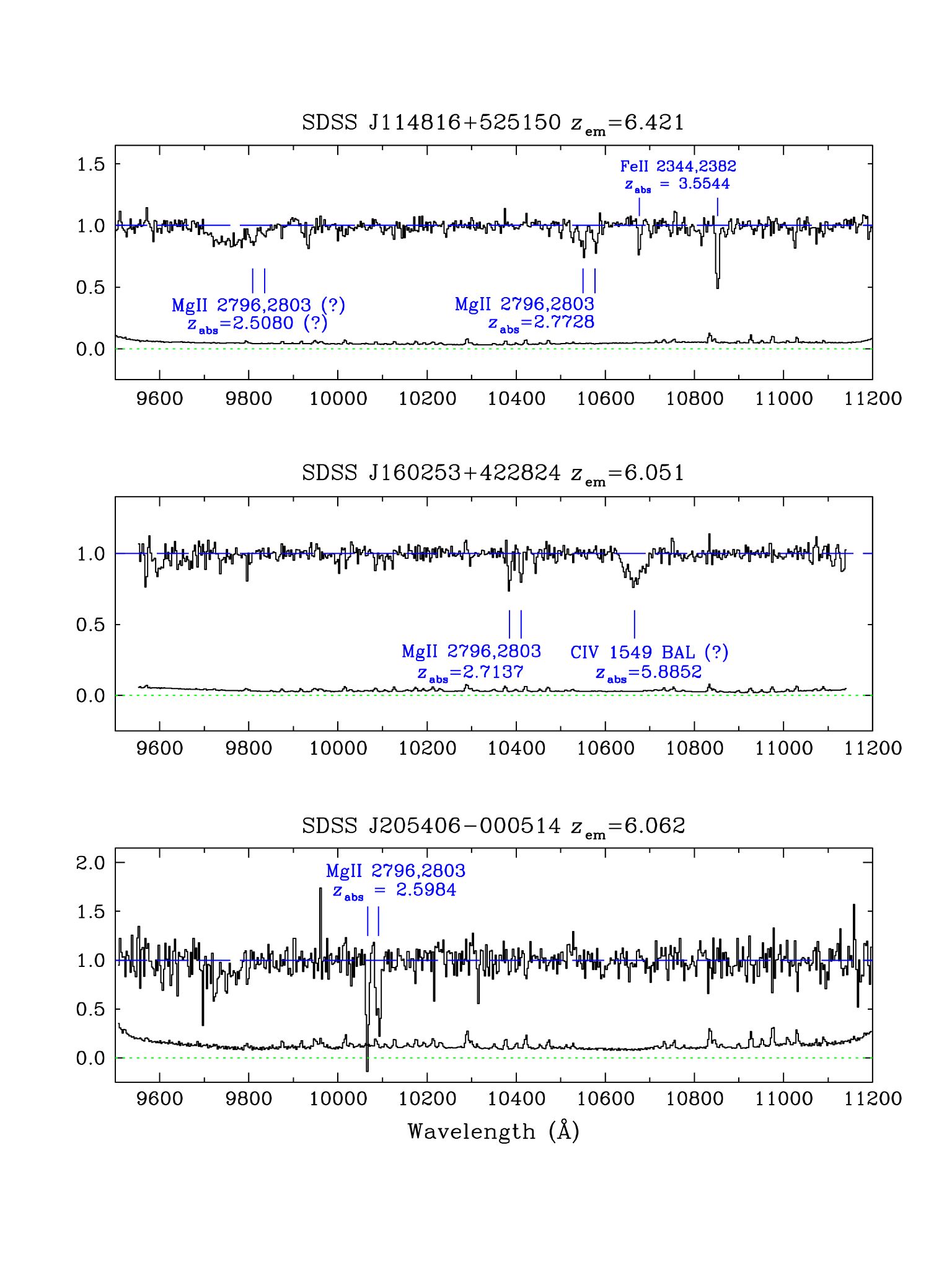
Figure 2: NIRSPEC spectra of SDSS J114816.64+525150.2, SDSS J160253.98+422824.9 and SDSS J205406.49$-$000514.8. In each panel, the top histogram shows the normalised QSO spectrum, while the lower histogram is the corresponding $1\sigma$ error spectrum. Absorption features are indicated by vertical tick marks and labelled with their identification.

2.2 ISAAC Observations

The ISAAC spectra were obtained with a mixture of service-mode and visitor-mode observations We used the instrument in its medium resolution mode with a 0.6 arcsec wide slit, which results in a spectral resolution ${\rm FWHM}=1.8$ Å (53 km s^-1), sampled with four pixels of the $1024\times 1024$ Hawaii Rockwell array. With this set-up, the wavelength range spanned is $\Delta\lambda\simeq 460$  Å; we normally chose a grating setting which placed the C iv emission line at the red limit of the range covered. In some cases, multiple wavelength settings were used, to increase the pathlength for absorption covered (see Table 1). The observations were conducted in the conventional ‘beam-switching’ mode, in a series of $4\times 900$ s exposures at two locations on the detector, typically separated by 10 arcsec. After each cycle of four integrations, the object was moved along the slit to a new pair of positions. The instrument was aligned on the sky at an angle chosen to include on the slit a bright star which provides a useful pointing and seeing reference.

The reduction of the ISAAC data used mainly IRAF tasks following the steps already described by Ryan-Weber et al. (2006). Briefly, we started from the ESO pipeline products which are 2-D images that have undergone a substantial amount of pre-processing, including flat-fielding, background subtraction, and wavelength calibration. Given the weakness of the sources at the moderately high dispersion of the ISAAC spectra, we found it most effective to combine all the processed frames of a given QSO (at a given wavelength setting) in 2-D, after appropriate shifts to bring them into alignment. This co-addition also allowed us to reject deviant pixels.

One-dimensional spectra were extracted from the co-added 2-D frames, with a second pass at subtracting any residual sky features; the data were then rebinned to two wavelength bins per resolution element in order to improve the S/N while still maintaining adequate spectral sampling. The final steps, including normalisation to the QSO continuum and estimate of the rms noise, were the same as described for the NIRSPEC spectra. As can be appreciated from inspection of Table 1, the values of S/N achieved with ISAAC tend to be lower than those of the NIRSPEC spectra, despite the generally longer integration times. However, the significantly higher spectral resolution provided by ISAAC, by a factor of $\sim 3.5$, largely compensates for the lower S/N, so that the two sets of data reach comparable sensitivities in terms of the minimum absorption line equivalent widths detectable.

     

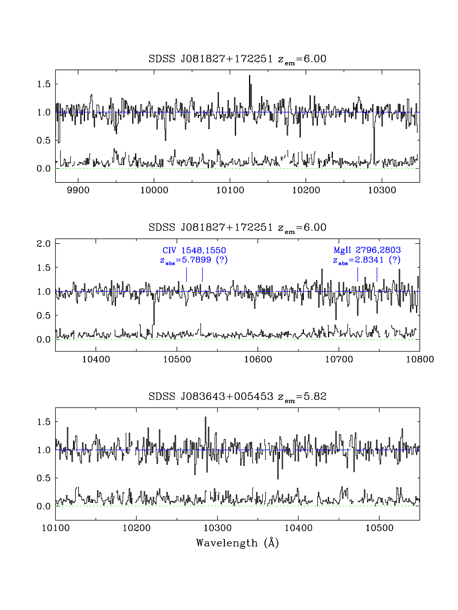
Figure 3: ISAAC spectra of SDSS J081827.40+172251.8 (two wavelength settings) and SDSS J083643.85+005453.3. In each panel, the top histogram shows the normalised QSO spectrum, while the lower histogram is the corresponding $1\sigma$ error spectrum. Absorption features are indicated by vertical tick marks and labelled with their identification. There is a tentative detection of an intervening C iv absorber towards SDSS J081827.40+172251.8 at $z_{\rm abs}=5.7899$; this possible system was omitted from the sample of definite detections used to estimate $\Omega_{\rm C\,\textsc{iv}}$.

     

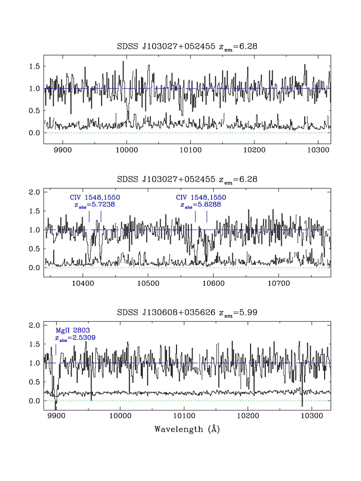
Figure 4: ISAAC spectra of SDSS J103027.01+052455.0 (two wavelength settings) and SDSS J130608.26+035626.3. In each panel, the top histogram shows the normalised QSO spectrum, while the lower histogram is the corresponding $1\sigma$ error spectrum. Absorption features are indicated by vertical tick marks and labelled with their identification. Parameters of the two C iv doublets identified towards SDSS J103027.01+052455.0 are listed in Tables 2 and LABEL:tab:abs.

3 Notes on individual QSOs

The normalised spectra of the ten QSOs in Table 1 are reproduced in Figures 1–4, together with the corresponding error spectra. Absorption lines were identified from a visual inspection of the spectra; they are labelled in Figures 1–4 and tabulated in Table 2. We now briefly comment on each QSO spectrum in turn.

3.1 ULAS J020332.38+001229.2

This QSO was identified by Venemans et al. (2007) from the first data release of the UKIRT Infrared Deep Sky Survey (UKIDSS), and independently by Jiang et al. (2008) from the Sloan Digital Sky Survey (SDSS). Both surveys reported similar emission redshifts: $z_{\rm em}=5.86$ (Venemans et al.) and $z_{\rm em}=5.854$ (Jiang et al.). From our NIRSPEC spectrum, however, we measure the lower value $z_{\rm em}=5.706$ from a broad emission feature which we presume to be C iv $\lambda 1549.062$; this value is in much better agreement with the recent reassessment of the optical and infrared spectrum of this source by Mortlock et al. (2008) who conclude that $z_{\rm em}=5.72$. Mortlock et al. point out that this is a broad absorption line (BAL) QSO which led the discoverers to misidentify the N v $\lambda 1240.1$ emission line as Ly$\alpha$: the latter is completely absorbed by the blueshifted N v absorption trough.

As this is a BAL QSO, we do not include it in the survey for C iv absorption (as we are primarily interested in C iv in the intergalactic medium, and wish to avoid contamination of our sample by metal-enriched gas which may be ejected from the QSO). Nevertheless, it is of interest to note that we do detect two narrow C iv doublets at redshifts $z_{\rm abs}=5.7541$ and $z_{\rm abs}=5.7961$ (see Figure 1); their equivalent widths are given in Table 2. Relative to $z_{\rm em}=5.706$, these two absorbers have velocities $v=+2150$ and $+4025$ km s^-1 and are thus most likely associated with the QSO environment. Positive velocities relative to $z_{\rm em}$ by up to $\sim 2000$–3000 km s^-1 have been encountered before among high ionisation absorbers at lower redshifts (e.g. Fox, Petitjean, & Bergeron 2008; Wild et al. 2008); the values we deduce here are rather extreme and may in part reflect the uncertainty in the systemic redshift $z_{\rm sys}$.

3.2 SDSS J081827.40+172251.8

This $z_{\rm em}=6.00$ QSO was observed with ISAAC at two wavelength settings which, together, cover the wavelength region 9877–10 790 Å with only a very small gap between them (see top two panels of Figure 3). We find two possible absorption systems: a C iv doublet at $z_{\rm abs}=5.7899$ and a Mg ii $\lambda\lambda 2796.3543,2803.5315$ doublet at $z_{\rm abs}=2.8341$; their reality can only be confirmed with higher S/N data.

Table 2: Absorption Lines Identified

QSO	$z_{\rm em}$	$z_{\rm abs}$	Ion	$\lambda_{\rm lab}^{a}$(Å)	$W_{0}$ (Å)	Comments
ULAS J020332.38+001229.2	5.706	5.7540	C iv	1548.2041	0.38	Intrinsic
		5.7543	C iv	1550.7812	0.25	Intrinsic
		5.7959	C iv	1548.2041	0.62	Intrinsic
		5.7962	C iv	1550.7812	0.56	Intrinsic
SDSS J081827.40+172251.8	6.00	5.7897	C iv	1548.2041	0.12	Tentative Identification
		5.7911	C iv	1550.7812	0.06	Tentative Identification
		2.8348	Mg ii	2796.3543	0.18	Tentative Identification
		2.8334	Mg ii	2803.5315	0.22	Tentative Identification
SDSS J084035.09+562419.9	5.774	5.5940	Si ii	1526.70698	0.52
		5.5938	Fe ii	1608.45085	0.34
		5.5943	Al ii	1670.7886	0.44
SDSS J103027.01+052455.0	6.28	5.7238	C iv	1548.2041	0.65
		5.7241	C iv	1550.7812	0.41
		5.8299:	C iv	1548.2041	…	$z_{\rm abs}$ and $W_{0}$ uncertain
		5.8299:	C iv	1550.7812	…	$z_{\rm abs}$ and $W_{0}$ uncertain
SDSS J113717.73+354956.9	5.962	5.0127	Al ii	1670.7886	0.70
		5.0120	Fe ii	1608.45085	0.65
		2.6260	Mg ii	2796.3543	0.52
		2.6261	Mg ii	2803.5315	0.55
		5.7380	C iv	1548.2041	0.33
		5.7387	C iv	1550.7812	0.20
SDSS J114816.64+525150.2	6.421	2.5077	Mg ii	2796.3543	0.56	Tentative Identification
		2.5084	Mg ii	2803.5315	0.29	Tentative Identification
		2.7727	Mg ii	2796.3543	0.77
		2.7728	Mg ii	2803.5315	0.60
		3.5545	Fe ii	2344.2139	0.34
		3.5544	Fe ii	2382.7652	0.96
SDSS J130608.26+035626.3	5.99	2.5309	Mg ii	2803.5315	2.50	$\lambda 2796.3543$ outside spectral rangec
SDSS J160253.98+422824.9	6.051	2.7138	Mg ii	2796.3543	0.44
		2.7135	Mg ii	2803.5315	0.38
SDSS J205406.49$-$000514.8	6.062	2.5973	Mg ii	2796.3543	2.05
		2.5995	Mg ii	2803.5315	2.29

^aFrom the compilation by Morton (2003).

^bThis value of equivalent width is in the observed frame (since the feature is unidentified).

^cBoth members of the doublet are present in the GNIRS spectrum published by Simcoe (2006).

3.3 SDSS J083643.85+005453.3

No absorption lines were identified in the $450$ Å stretch of the near-IR spectrum of this QSO recorded with ISAAC (see bottom panel of Figure 3).

3.4 SDSS J084035.09+562419.9

Our NIRSPEC spectrum of this QSO includes the broad C iv emission line at redshift $z_{\rm em}=5.774$, to be compared with the SDSS value $z_{\rm em}=5.85\pm 0.02$ reported by Fan et al. (2006b). We find no C iv systems, but we do detect three absorption lines from a low ionisation system at $z_{\rm abs}=5.5940$ (middle panel of Figure 1, and Table 2). It would be of great interest to determine the metallicity (and other physical parameters) of such high redshift absorbers which may be associated with neutral gas in galaxies; however, it is hard to envisage how this can be accomplished, given that the associated Lyman series lines are essentially indistinguishable against the backdrop of the nearly-black Ly$\alpha$ forest.

Table 3: Parameters of identified C iv absorption systems

QSO	Instrument	$z_{\rm abs}$	$\log N$(C iv)/cm-2)	$b$ (km s-1)	Comments
SDSS J103027.01+052455.0	ISAAC	$5.7238\pm 0.0001$	$14.39\pm 0.05$	$61\pm 6$
SDSS J103027.01+052455.0	ISAAC	$5.8288\pm 0.0002$	$14.45\pm 0.13$	$26\pm 9$
SDSS J113717.73+354956.9	NIRSPEC	$5.7383\pm 0.0002$	$14.20\pm 0.15$	$30\pm 12$
SDSS J081827.40+172251.8	ISAAC	$5.7899\pm 0.0003$	$13.57\pm 0.16$	$39\pm 25$	Tentative identification

3.5 SDSS J103027.01+052455.0

This was the first QSO to be observed as part of this programme and a portion of its spectrum was published by Ryan-Weber et al. (2006). In Figure 4 we show the full ISAAC spectrum which extends from 9880 Å to 10 780 Å, recorded with three, partially overlapping, grating settings. We find two strong C iv doublets, at $z_{\rm abs}=5.7238$ and 5.8288. The latter was considered as marginal by Ryan-Weber et al. (2006), but independent observations by Simcoe (2006) with the Gemini Near-Infrared Spectrograph (GNIRS) confirm its reality. Even so, it is difficult with the quality of our data to measure the equivalent widths of the two C iv lines in this absorber, as they appear to be blended with other broader features.

3.6 SDSS J113717.73+354956.9

This is one of our best NIRSPEC spectra (see Figure 1). The emission redshift we determine from C iv $\lambda 1549.062$, $z_{\rm em}=5.962$, is lower than the value $z_{\rm em}=6.01\pm 0.02$ reported by Fan et al. (2006b) from the discovery SDSS spectrum. We identify absorption lines from three separate systems in the 1630 Å portion of the spectrum recorded with NIRSPEC: a high redshift, low ionisation system at $z_{\rm abs}=5.0124$, a Mg ii absorber at $z_{\rm abs}=2.6261$, and a C iv doublet at $z_{\rm abs}=5.7383$. The equivalent widths of all these lines are given in Table 2.

3.7 SDSS J114816.64+525150.2

This is the highest redshift QSO in the present sample. We measure $z_{\rm em}=6.421$ from the Si iv $\lambda 1396.752$ broad emission line, in good agreement with the value $z_{\rm em}=6.42$ published by Fan et al. (2006c). Our NIRSPEC spectrum (top panel of Figure 2) shows a definite Mg ii doublet at $z_{\rm abs}=2.7728$, and a possible one at $z_{\rm abs}=2.5080$ which appears to be part of a broad feature of uncertain identity. We also cover two Fe ii lines, $\lambda\lambda 2344,2382$, in a strong low ionisation system at $z_{\rm abs}=3.5544$; other Fe ii and Mg ii lines in this system can be recognised in the spectrum published by Barth et al. (2003).

3.8 SDSS J130608.26+035626.3

The relatively short integration (two hours) of this object with ISAAC resulted on a relatively noisy spectrum (S/N $\simeq 5$) reproduced in the bottom panel of Figure 4 and already reported by Ryan-Weber et al. (2006). No C iv doublets are detected. The strong absorption line present in the spectrum is the longer wavelength member of the Mg ii $\lambda\lambda 2796.3543,2803.5315$ doublet at $z_{\rm abs}=2.5309$; both lines can be discerned in the GNIRS spectra of this object obtained independently by Simcoe (2006) and by Jiang et al. (2007).

3.9 SDSS J160253.98+422824.9

Our measured $z_{\rm em}=6.051$ is in reasonable agreement with $z_{\rm em}=6.07$ from the SDSS (Fan et al. 2006c). We detect a definite Mg ii system at $z_{\rm abs}=2.7137$, as well as a puzzling broad absorption feature (see middle panel of Figure 2). If this were a C iv ‘mini-BAL’, its ejection velocity relative to $z_{\rm em}$ would be 7150 km s^-1.

3.10 SDSS J205406.49$-$000514.8

Even a relatively short exposure (5400 s) with NIRSPEC is sufficient to reveal the very strong Mg ii doublet present at $z_{\rm abs}=2.5984$ (bottom panel of Figure 2). This Mg ii absorber, and the one at $z_{\rm abs}=2.5309$ in SDSS J130608.26+035626.3, are close to the threshold for classification as “Ultra-Strong Systems” in the SDSS survey by Nestor, Turnshek, & Rao (2005). It is interesting to note that these authors find a steep redshift evolution in the frequency of such systems, which become progressively rarer at $z\lower 2.15277pt\hbox{$\;\buildrel<\over{\sim}\;$}1$.

4 Survey for intergalactic C iv at $z>5$

4.1 Redshift Range Sampled

In the last column of Table 1 we have listed for each QSO the redshift intervals over which we searched for C iv absorption. The values of $z_{\rm min}$, which range from 5.16 to 5.52, correspond to wavelengths close to the values of $\lambda_{\rm min}$ in column (5) for the detection of $\lambda 1548.2041$. The values of $z_{\rm max}$, which range from 5.66 to 6.20, correspond either to wavelengths close to the values of $\lambda_{\rm max}$ in column (5) for the detection of $\lambda 1550.7812$, or to $z_{\rm em}-3000$ km s^-1, whichever is the lower [the QSO emission redshifts are listed in column (3)]. We exclude ‘proximate systems’ within 3000 km s^-1 of the emission redshift because they may be associated with the QSO environment, rather than with the more generally distributed IGM; however, none were found in the present survey except for the two systems in ULAS J020332.38+001229.2 which is not included in the analysis anyway as it is a BAL QSO (see section 3.1).

From these values of $z_{\rm min}$ and $z_{\rm max}$ we calculate the corresponding absorption distances, given by:

$$X(z)={2\over 3\Omega_{\rm M}}\,\{[\Omega_{\rm M}(1+z)^{3}+\Omega_{\Lambda}]^{1/2}-1\}$$ (1)

which is valid for $\Omega_{\rm M}+\Omega_{\Lambda}=1$, where $\Omega_{\rm M}$ and $\Omega_{\Lambda}$ are respectively the matter and vacuum density parameters today. With $\Omega_{\rm M}=0.3$ and $\Omega_{\Lambda}=0.7$, we find that our survey covers a total absorption distance $\Delta X=25.1$.

4.2 C iv Column Densities

Summarising the results of section 3, we find three definite and one possible C iv doublets over this absorption distance. We deduced values of column density $\log N$(C iv)/cm^-2 for these absorbers by fitting the observed absorption lines with theoretical Voigt profiles generated by the vpfit package. For each absorber, vpfit determines the most likely values of redshift $z_{\rm abs}$, Doppler width $b$ (km s^-1), and column density $\log N$(C iv)/cm^-2, by minimizing the difference between the observed line profiles and theoretical ones convolved with the instrumental point spread function. Vacuum rest wavelengths and $f$-values of the C iv transitions are from the compilation by Morton (2003). For an illustrative use of this line-fitting software, see Rix et al. (2007).

Table LABEL:tab:abs lists the values returned by vpfit, together with their $1\sigma$ errors, for the four C iv absorbers considered here. Strictly speaking, these values of $N$(C iv) are lower limits to the true column densities because at the relative coarse spectral resolution of our data the absorption lines we see are likely to be the unresolved superpositions of several components (e.g. Ellison et al. 2000), some of which may be saturated. This concerns applies particularly to the $z_{\rm abs}=5.7383$ doublet in SDSS J113717.73+354956.9 for which the $b$ value on which vpfit converged ($b=30$ km s^-1, to be interpreted as an ‘equivalent’ velocity dispersion parameter describing the ensemble of components) is much smaller than the NIRSPEC instrumental broadening $b_{\rm instr}=110$ km s^-1—in other words, these doublet lines are totally unresolved. On the other hand, the doublet ratio $W(1548)/W(1550)=1.65$ is consistent with only a moderate degree of line saturation. In the other three cases, the equivalent $b$-values are comparable to, or larger than, $b_{\rm instr}=32$ km s^-1 of ISAAC (see Table LABEL:tab:abs), indicating that the C iv absorption lines are partially resolved. For the remainder of our analysis, we shall assume that the column densities of C iv have not been underestimated by large factors, although this assumption will need to be verified in future with higher resolution observations.

4.3 Mass density of C iv

It has become customary to express the mass density of an ion (in this case C iv) as a fraction of the critical density today:

$$\Omega_{\rm C\,\textsc{iv}}=\frac{H_{0}\,m_{\rm C\,\textsc{iv}}}{c\,\rho_{\rm crit}}\int Nf(N){\rm d}N,$$ (2)

where $H_{0}=100\,h$ km s^-1 Mpc^-1 is the Hubble constant, $m_{\rm C\,\textsc{iv}}$ is the mass of a C iv ion, $c$ is the speed of light, $\rho_{\rm crit}=1.89\times 10^{-29}\,h^{2}$ g cm^-3, and $f(N)$ is the number of C iv absorbers per unit column density per unit absorption distance $X(z)$. In the absence of sufficient statistics to recover the column density distribution function $f(N)$, as is the case here, the integral in eq. (2) can be approximated by a sum:

$$\int Nf(N){\rm d}N=\frac{\sum_{i}N_{i}{\rm(C\,\textsc{iv})}}{\Delta X}$$ (3)

with an associated fractional variance:

$$\left(\frac{\delta\Omega_{\rm C\,\textsc{iv}}}{\Omega_{\rm C\,\textsc{iv}}}\right)^{2}=\frac{\sum_{i}[N_{i}{\rm(C\,\textsc{iv})}]^{2}}{\left[\sum_{i}N_{i}{\rm(C\,\textsc{iv})}\right]^{2}},$$ (4)

as proposed by Storrie-Lombardi, McMahon, & Irwin (1996). With $h=0.70$, eqs. (2) and (3) then lead to:

$$\Omega_{\rm C\,\textsc{iv}}=1.63\times 10^{-22}~{}\frac{\sum_{i}N_{i}{\rm(C\,\textsc{iv})}}{\Delta X}.$$ (5)

Summing up the values of $N_{i}$(C iv) in Table LABEL:tab:abs and dividing by $\Delta X=25.1$, we find:

$$\Omega_{\rm C\,\textsc{iv}}=(4.4\pm 2.6)\times 10^{-9}$$ (6)

over the redshift interval $z_{\rm abs}=5.2$–6.2 at a mean $\langle z_{\rm abs}\rangle=5.76$. We have not included the possible system at $z_{\rm abs}=5.7899$ in the summation; its inclusion would increase $\Omega_{\rm C\,\textsc{iv}}$ by only $5\%$. For comparison, Pettini et al. (2003) measured $\Omega_{\rm C\,\textsc{iv}}=(2.2\pm 0.8)\times 10^{-8}$ at $\langle z_{\rm abs}\rangle=4.69$ (in the same cosmology as adopted here); these two values, together with the lower redshift determinations by Songaila (2001), are plotted in Figure 5.

Thus, at first sight, $\Omega_{\rm C\,\textsc{iv}}$ seems to have dropped by about a factor of five in only $\sim 300$ Myr, as we move back in time from $z\sim 4.7$ to $z\sim 5.8$. However, before we can be confident of such a rapid build-up of C iv at these early epochs in the Universe history (these redshifts correspond to only $\sim 1$ Gyr after the Big Bang—see top axis of Figure 5), we have to look carefully at the different completeness limits of the surveys whose results are collected in Figure 5. In particular, the sensitivities of absorption line searches at near-IR wavelengths, such as the one reported here, are still lower than those achieved at optical wavelengths with comparable observational efforts and we suspect that this difference must be contributing to some extent to the high redshift drop evident in Figure 5.

 

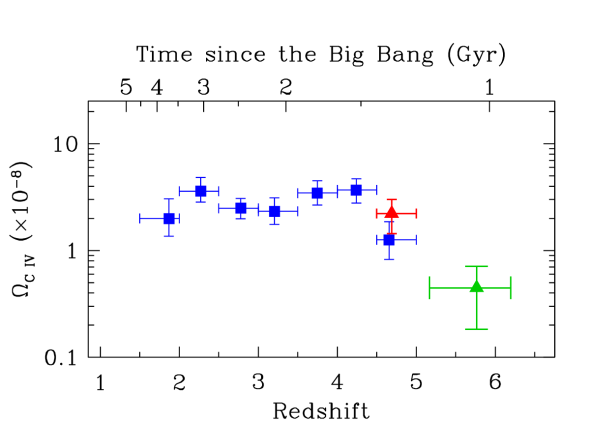
Figure 5: Cosmological mass density of C iv as a function of redshift. The blue squares show the measurements by Songaila (2001), the red triangle is from Pettini et al. (2003), and the green triangle is the value deduced here. All values plotted have been reduced to the ‘737’ cosmology adopted in the present work. Error bars are $1\sigma$. While this plot shows the actual values of $\Omega_{\rm C\,{\textsc{i}v}}$ measured, they are not strictly comparable because each of the three surveys had a different sensitivity limit. This issue is discussed in detail in the text (section 5).

5 Completeness Limit of the Survey

In order to quantify this effect, we conducted a series of Monte Carlo simulations, as follows. We used vpfit to generate theoretical C iv doublets for ranges of values of $b$ and $N$(C iv); these fake absorption lines were then inserted at random redshifts into the real spectra, after convolution with the appropriate instrumental profile (depending on whether the spectrum to be ‘contaminated’ was a NIRSPEC or an ISAAC one) and with random noise reflecting the measured S/N of the spectrum at that wavelength. We then tested whether we could recover these C iv doublets by visual inspection of the spectra, in the same way as the real absorbers were identified. So as to test the sensitivity of our survey as comprehensively as practical, we chose three sets of values for the velocity dispersion parameter, $b=20$, 40 and 60 km s^-1, reflecting the range of $b$-values of the real C iv doublets (see Table LABEL:tab:abs). For the column density we considered twelve values, in 0.1 dex steps between $\log N({\rm C\,\textsc{iv})/cm}^{-2}=13.4$ and 14.5. For each combination of $b$ and $\log N({\rm C\,\textsc{iv}})$, we created 40 Monte Carlo realisations, so that the full series of completeness tests involved 1440 fake C iv doublets distributed within our parameter space.

 

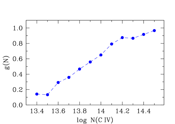
Figure 6: Sensitivity function to C iv doublets in our survey, deduced from 1440 Monte Carlo realisations. See text (section 5) for further details.

We found that the fraction of C iv doublets recovered, $g(N)$, did not depend sensitively on $b$ nor $z_{\rm abs}$ but, as expected, was a function of column density—see Figure 6. While we seem to be $\sim 90\%$ complete for column densities $\log N({\rm C\,\textsc{iv})/cm}^{-2}\geq 14.2$, our sensitivity drops fairly rapidly below this value: we can only detect about half of the C iv doublets with half this column density and, if $N$(C iv) drops by a further factor of two, we miss some 85% of the absorbers. For comparison, the estimate of $\Omega_{\rm C\,\textsc{iv}}$ by Pettini et al. (2003) refers to C iv absorbers with $\log N({\rm C\,\textsc{iv})/cm}^{-2}\geq 13.0$ (and includes a 22% correction for the fall in completeness of their Keck-ESI spectra from $\sim 100\%$ at $\log N({\rm C\,\textsc{iv})/cm}^{-2}\geq 13.3$ to 45% at $\log N({\rm C\,\textsc{iv})/cm}^{-2}=13.0$). Songaila’s (2001) estimates of $\Omega_{\rm C\,\textsc{iv}}$, on the other hand, refer to the yet wider column density interval $12.0\leq\log N({\rm C\,\textsc{iv})/cm}^{-2}\leq 15.0$ which she could access thanks to the high spectral resolution and S/N of her Keck-HIRES spectra. From her Figure 1, it appears that her number counts become progressively less complete below $\log N({\rm C\,\textsc{iv})/cm}^{-2}\simeq 13.0$, although no correction was applied to account for this.

From the above discussion it is evident that, in order to assess the significance of the suggested drop in $\Omega_{\rm C\,\textsc{iv}}$ beyond $z\simeq 4.7$, we need to consider the results of these different surveys over the same range of C iv column densities. Referring to Figure 5, we see that we are $>50\%$ complete for $\log N({\rm C\,\textsc{iv})/cm}^{-2}\geq 13.8$, so that we can compare with the surveys by Songaila (2001) and Pettini et al. (2003) in this column density regime. Specifically, we have adjusted the values $\Omega_{\rm C\,\textsc{iv}}$ reported by those authors as follows:

$$\Omega^{\prime}_{\rm C\,\textsc{iv}}=\Omega_{\rm C\,\textsc{iv}}\times\frac{\int^{{10}^{15.0}}_{{10}^{13.8}}Nf(N){\rm d}N}{\int^{{10}^{15.0}}_{{10}^{12.0}}Nf(N){\rm d}N}$$ (7)

for the values published by Songaila (2001), and

$$\Omega^{\prime}_{\rm C\,\textsc{iv}}=\Omega_{\rm C\,\textsc{iv}}\times\frac{\int^{{10}^{15.0}}_{{10}^{13.8}}Nf(N){\rm d}N}{\int^{{10}^{15.0}}_{{10}^{13.0}}Nf(N){\rm d}N}$$ (8)

for the value published by Pettini et al. (2003), assuming

$$f(N)=10^{-12.65}N_{13}^{-1.8},$$ (9)

where $N_{13}$ is $N$(C iv) in units of $10^{13}$ cm^-2, as determined by Songaila (2001).

The lower limits of integration in the denominators of eqs. (7) and (8) reflect the sensitivity limits of the corresponding surveys. Since the survey by Songaila (2001) is only partially complete for C iv absorbers with $12.0\leq\log N({\rm C\,\textsc{iv})/cm}^{-2}\leq 13.0$, eq. (7) may overestimate the correction required—this works in the sense of diluting the evidence for a drop in $\Omega_{\rm C\,\textsc{iv}}$ at higher redshifts. The effect is most pronounced for the highest redshift bin in Songaila’s sample, because her data is least sensitive to column densities $\log N({\rm C\,\textsc{iv})/cm}^{-2}<13.0$ at $z_{\rm abs}\geq 4.5$ (see Figure 2 of Songaila 2001); accordingly we have indicated her highest redshift data point with a different colour in Figure 7.

For the NIRSPEC+ISAAC sample presented here, we have modified eq. (5) to include our sensitivity function $g(N)$ shown in Figure 6:

$$\Omega^{\prime}_{\rm C\,\textsc{iv}}=1.63\times 10^{-22}~{}\frac{\sum_{i}N_{i}{\rm(C\,\textsc{iv})}\times g(N_{i})}{\Delta X}.$$ (10)

All the errors have been scaled accordingly, so as to maintain the same percentage error.

 

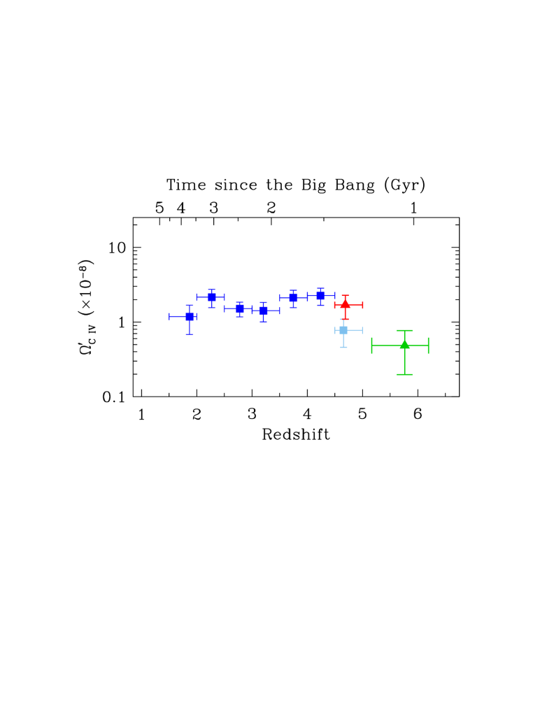
Figure 7: Cosmological mass density of C iv as a function of redshift, taking into account only C iv absorbers with column densities $13.8\leq\log N({\rm C\,\textsc{iv})/cm}^{-2}\leq 15.0$, to which all three surveys considered here are sensitive. The symbols have the same meaning as in Figure 5. For the highest redshift data point in the sample by Songaila (2001), shown by the pale blue square, the correction of eq. (7) probably underestimates the value of $\Omega^{\prime}_{\rm C\,\textsc{iv}}$.

Values of $\Omega^{\prime}_{\rm C\,\textsc{iv}}$ are plotted in Figure 7. Evidently, we still see a drop in the mass density of C iv as we look back beyond $z\simeq 4.7$, albeit at a reduced significance compared to Figure 5. Considering only absorbers with $\log N({\rm C\,\textsc{iv})/cm}^{-2}\geq 13.8$, we find that $\Omega^{\prime}_{\rm C\,\textsc{iv}}$ decreases by factor of $\sim 3.5$, as we move from $\Omega^{\prime}_{\rm C\,\textsc{iv}}=(1.7\pm 0.6)\times 10^{-8}$ at $\langle z\rangle=4.69$ to $\Omega^{\prime}_{\rm C\,\textsc{iv}}=(5\pm 3)\times 10^{-9}$ at $\langle z\rangle=5.76$ ($1\sigma$ errors). The drop is significant at the $4\sigma$ level.

6 Absorption Line Statistics

We can examine the evidence for a decrease in intergalactic C iv at redshifts $z>4.7$ in an alternative way from considering simply the sum of their column densities. It is instructive to ask how the number of detected C iv doublets compares with the number we may have expected under the assumption of an invariant column density distribution, $f(N)$. Again, we assume $f(N)=10^{-12.65}N_{13}^{-1.8}$ (Songaila 2001), which implies $f(>N)=2.8\,N_{13}^{-0.8}$ per unit absorption distance.

Our survey is not uniform in either S/N nor resolution, and both factors determine the minimum value of $N$(C iv) detectable. We therefore calculated the expected value of $f(>N)$ on a spectrum by spectrum basis, using as threshold the $5\sigma$ detection limit for the equivalent width of an absorption line:

$$W_{0}(5\sigma)=\frac{5\delta\lambda}{1+z}\times\frac{1}{\rm{S/N}}$$ (11)

where $\delta\lambda$ is the resolution in Å. Values of resolution and S/N for each spectrum are listed in Table 1. With $W_{0}(5\sigma)$ is associated a minimum column density:

$$N_{\rm C\,\textsc{iv}}(5\sigma)=1.13\times 10^{20}\times\frac{W_{0}(5\sigma)}{\lambda^{2}f}~{}{\rm cm}^{-2}$$ (12)

where $\lambda$ and $W_{0}$ are both in Å and $f$ is the oscillator strength of the transition (in this case C iv$\lambda 1550.7812$, the weaker member of the doublet).

In Figure 8 we plot the cumulative number of absorbers expected (for the minimum column density to which each spectrum is sensitive) as a function of the cumulative pathlength. Over our total survey pathlength, $\Delta X=25.1$, we expect to detect $10^{+3}_{-5}$ C iv absorbers. We instead find three absorbers, indicating that the distribution of C iv column densities which applies at redshift $1.5\leq z\leq 4.5$ does not continue unchanged to $5.2\leq z\leq 6.2$. The likelihood of detecting three C iv systems when ten are expected is less than 1%. It is interesting to note that the absorption systems we do detect were found in spectra with column density sensitivities in the middle of the range of our survey: $N_{\rm C\,\textsc{iv}}(5\sigma)=9.1\times 10^{13}$ cm^-2 and $1.2\times 10^{14}$ cm^-2 for SDSS J113717.73+354956.9 and SDSS J103027.01+052455.0 respectively. The absorber towards SDSS J113717.73+354956.9 represents a $6.6\sigma$ detection. Thus, it seem unlikely that we are missing a considerable number of absorption systems above our $5\sigma$ sensitivity limit.

 

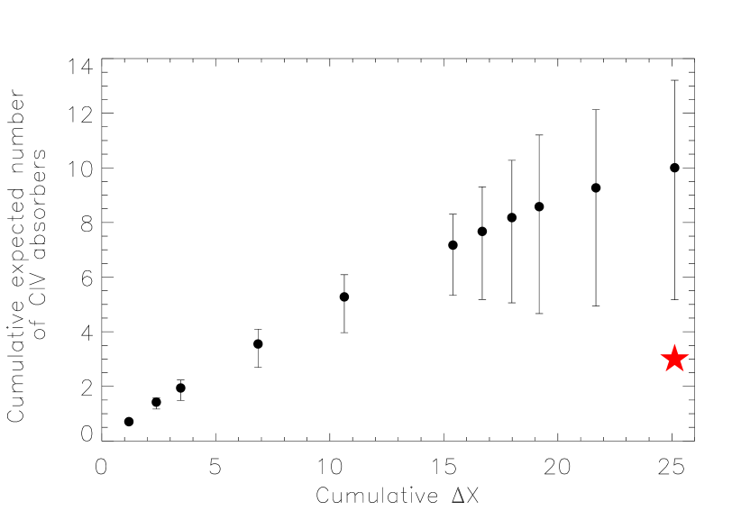
Figure 8: Cumulative number of C iv absorption systems expected from our survey (if there is no evolution in the column density distribution function from redshift $z\sim 3$ to 6). The cumulative number is plotted as a function of the survey pathlength, $\Delta X$, which increases as each spectrum is added to data set. We expect to find 10 C iv absorption systems in our total pathlength of $\Delta X=25.1$. The star symbol denotes the three absorbers we detect in our entire survey in the redshift range $5.2<z<6.2$.

7 Discussion

To summarise, by extending our previous searches for intergalactic C iv to near-IR wavelengths, we have found that both the number of such absorbers per unit absorption distance and the comoving mass of triply ionised carbon are approximately three times lower at $z\simeq 5.8$ than at $z<4.7$. Although our results refer to the stronger C iv systems in the column density distribution function, with $\log N{\rm(C\,\textsc{iv})/cm}^{-2}\geq 13.8$, the evolution appears to extend at least to absorbers with half this column density (Becker et al. 2009).

Before considering the implications of these results, we reflect briefly on possible caveats. As already mentioned, we may have underestimated the column densities of C iv through line saturation; we do not expect this effect to be so severe as to cause (spuriously) the fall in $\Omega_{\rm C\,\textsc{iv}}$ evident in Figure 7, but only higher resolution observations will quantify the corrections required (if any). It must also be borne in mind that the distribution of C iv at $z>5.2$ seems to be extremely patchy: of the nine sight-lines sampled, seven show no absorption, while two absorbers are found in the direction of one QSO. Thus, our statistics are very prone to what in galaxy counts is referred to as ‘cosmic variance’. This can explain why the pilot observations by Ryan-Weber et al. (2006) suggested a higher value of $\Omega_{\rm C\,\textsc{iv}}$–the first stage of our survey fortuitously found one-third of the $\sum_{i}N_{i}\rm(C\,\textsc{iv})$ of the whole sample presented here, even though it covered only $\sim 15\%$ of the total $\Delta X$. Conversely, Becker et al. (2009) detected no absorbers in their higher resolution NIRSPEC spectra of four QSOs (three in common with our sample) over less than half of the $\Delta X$ of our survey. In future, better statistics will undoubtedly improve the accuracy of determinations of $\Omega_{\rm C\,\textsc{iv}}$ at $z>5$; for the moment we shall proceed on the assumption that our estimate of the error on this quantity, as shown in Figure 7, is realistic.

The downturn in $\Omega_{\rm C\,\textsc{iv}}$ we have discovered as we approach $z\sim 6$ is clear evidence of important changes taking place in the Universe at, or before, this epoch. In the following discussion we shall find it more convenient to ‘turn the time arrow around’, and to think of the evolution as time progresses from higher to lower redshifts. The rise in $\Omega_{\rm C\,\textsc{iv}}$ we see in Figure 7 could result either from an increase in the amount of intergalactic carbon, or from changes in the ionisation balance favouring the fraction of carbon which is triply ionised, or both. Indeed, there are indications from previous work that both effects may be at play.

By integrating the galaxy luminosity function down to 1/5 of the fiducial luminosity at $z=3$ (that is, considering galaxies with $L\geq 0.2\,L^{\ast}_{z=3}$), Bouwens et al. (2008) found that the cosmic star-formation rate density increased by a factor of $\lower 2.15277pt\hbox{$\;\buildrel>\over{\sim}\;$}4$ over the 400 Myr period from $z=9$ to $z=6$. The growth in intergalactic C iv we see at $z<6$ may well be a reflection of this enhanced star-formation activity, as the products of stellar nucleosynthesis accumulate in the IGM, presumably transported by galactic outflows. Note that this is carbon produced by massive stars, with evolutionary time-scales of less than 10 Myr (Pettini et al. 2008b; Pettini 2008); it is therefore quite conceivable that over $\sim 400$ Myr the products of Type II supernovae could have travelled considerable distances from their production sites.

On the other hand, Fan et al. (2006c) have argued for a marked increase in the transmission of the Ly$\alpha$ forest at $z\lower 2.15277pt\hbox{$\;\buildrel<\over{\sim}\;$}6$, which has been interpreted as marking the overlap of the hydrogen ionisation fronts from star-forming galaxies, as the IGM became transparent to Lyman continuum photons (e.g. Gnedin & Fan 2006). Opinions are still divided, however, as to the correct interpretation of the Ly$\alpha$ forest evolution at these high redshifts (e.g. Becker, Rauch, & Sargent 2007 and references therein). Coupled with the rise in the comoving density of bright QSOs (Fan 2006), a higher IGM transmission would quickly ionise a larger fraction of carbon into C iv.

To make progress beyond these qualitative remarks, detailed modelling is necessary. As mentioned in the Introduction, B. Oppenheimer and collaborators have devoted considerable attention to this problem and shown, in particular, how momentum-driven winds from star-forming galaxies can reproduce the behaviour of $\Omega_{\rm C\,\textsc{iv}}$ at redshifts $z<5$. It is therefore of interest to consider their model predictions for earlier epochs. Their latest models (Oppenheimer, Davé, & Finlator 2009) do indeed entertain a marked growth in $\Omega_{\rm C\,\textsc{iv}}$ from $z=8$ to 5, driven by both effects mentioned above. In their scenario, the overall density of carbon increases by a factor of $\sim 2$ between $z=5.8$ and 4.7. The accompanying rise in $\Omega_{\rm C\,\textsc{iv}}$ depends on the spectral shape of the radiation field which dominates the ionisation equilibrium. Oppenheimer et al. (2009) consider two possibilities: the metagalactic background in the formulation by Haardt & Madau (1996) with recent updates, and a more local field dominated by early-type stars in the nearest galaxy to the C iv absorbers, in recognition of the fact that cosmic reionisation was likely to be very patchy at these early epochs. The former produces the larger change in $\Omega_{\rm C\,\textsc{iv}}$ (for the reasons explained above), which grows by a factor of $\sim 5$ between $z=5.8$ and 4.7; the latter results in a more modest rise, by a factor of $\sim 2-3$.

Given our warnings about the effects of ‘cosmic variance’ on the current observational determinations of $\Omega_{\rm C\,\textsc{iv}}$, it would be quite premature to compare in detail these theoretical predictions with the data in Figure 7 and, for example, draw conclusions on the shape of the ionising background at these early epochs. It is encouraging, nevertheless, that models and data concur in a general trend towards a build-up of C iv over the relatively short cosmic period between $z\sim 6$ and 5. Two ingredients of the simulations by Oppenheimer et al. (2009) need to be clarified, however. The first, and more important one, is that in their scenario the galaxies responsible for most of the IGM enrichment are of low mass and with luminosities well below the current observational limit $L\geq 0.2\,L^{\ast}_{z=3}$. We know very little, if anything at all, about the galaxies at the faint end of the luminosity function at $z>5$, and this situation is unlikely to be remedied until the launch of the James Webb Space Telescope in the next decade. A second concern is the resonant opacity of the IGM at the frequencies of the He ii Lyman series which has been neglected until recently, and which may affect the distribution of carbon among its highly ionised states (Madau & Haardt 2009).

7.1 Reionization

The average metallicity of the IGM at a given epoch reflects the accumulation of the heavy elements synthesised by previous generations of stars and expelled from their host galaxies. The massive stars which explode as Type II supernovae and seed the IGM with metals are also the sources of nearly all of the Lyman continuum photons produced by a burst of star formation. Consequently, it is relatively straightforward to link a given IGM metallicity with a minimum number of LyC photons which must have been produced up until that time. The close correspondence between the sources metals and photons makes the conversion from one to the other largely independent of the details of the stellar initial mass function (IMF). For example, Madau & Shull (1996) calculate that changing the index of a power-law formulation of the IMF, such as Salpeter’s (1955), from $\alpha=2$ to 3, results in only a 10% difference in the conversion between metallicity and number of LyC photons emitted.

When in the past this line of reasoning has been applied to measures of the IGM metallicity at $z\sim 3$ (e.g. Madau & Shull 1996; Miralda-Escude & Rees 1997), it has been concluded that the star formation activity prior to that epoch probably produced sufficient photons to reionise the Universe. With our new estimate of $\Omega_{\rm C\,\textsc{iv}}$, much closer in time to what may have been the end of the process of reionisation, we are able to revisit this question more critically.

We begin by calculating the IGM metallicity by mass, $Z_{\rm IGM}$, implied by our measure of $\Omega_{\rm C\,\textsc{iv}}$:

$$Z_{\rm IGM}=\frac{\mbox{$\Omega_{\rm C\,\textsc{iv}}$}}{\Omega_{\rm b}}\cdot\frac{\rm C_{\rm{TOT}}}{\rm C\,{\textsc{iv}}}\cdot\frac{1}{A_{\rm C}}$$ (13)

where $\Omega_{\rm b}=0.0224/h^{2}$ (Pettini et al. 2008a) is the contribution of baryons to the critical density, $\rm C\,{\textsc{iv}}/\rm C_{\rm{TOT}}$ is the fraction of carbon which is triply ionised, and $A_{\rm C}$ is the mass fraction of metals in carbon. For comparison, in the Sun, $Z_{\odot}=0.0122$ and $A_{\rm C}=0.178$ (Asplund, Grevesse, & Sauval 2005); here we assume that the same value of $A_{\rm C}$ applies at high redshifts because: (a) the ratio of carbon to oxygen (the major contributor to $Z_{\odot}$) is approximately solar at low metallicities (Pettini et al. 2008b; Fabbian et al. 2009); and (b) any departures are in any case likely to result in only a small correction compared to other uncertainties in the following discussion. We also adopt the conservative limit ${\rm C\,\textsc{iv}}/{\rm C_{\rm{TOT}}}\leq 0.5$, as done by Songaila (2001); this is the maximum fractional abundance reached by C iv under the most favourable ionisation balance conditions. With these parameters, our measured

$$\Omega_{\rm C\,\textsc{iv}}=(4.4\pm 2.6)\times 10^{-9}$$ (14)

implies

$$Z_{\rm IGM}=(1.1\pm 0.6)\times 10^{-6}=(9\pm 5)\times 10^{-5}\,Z_{\odot}.$$ (15)

In recent years, much theoretical attention has been directed to estimating the likely properties of metal-poor early-type stars. Schaerer (2002) pointed out that stellar luminosities at far-UV wavelengths are higher at lower metallicities, leading to a greater output of LyC photons associated with stellar nucleosynthesis. Specifically, the energy emitted in hydrogen ionising photons (per baryon) is related to the average cosmic metallicity by:

$$E_{\rm Z}=\eta\,m_{\rm p}c^{2}\,\langle Z\rangle\,{\rm MeV}$$ (16)

where $m_{\rm p}c^{2}=938$ MeV is the rest mass of the proton and $\eta$ is the stellar efficiency conversion factor. Schaerer (2002) estimated $\eta=0.014$ for stars with $Z=1/50Z_{\odot}$, a factor of $\sim 4$ higher than at solar metallicities (see also Venkatesan & Truran 2003). For an average energy of 21 eV per LyC photon (Schaerer 2002), our determination of $\langle Z_{\rm IGM}\rangle=1.1\times 10^{-6}$ then implies that less than one ($\sim 0.7$) LyC photon per baryon was emitted by early-type stars prior to $z=5.8$.

This background is clearly insufficient to keep the Universe ionised. When we take into account that: (a) an unknown fraction, $f_{\rm esc}<1$, of the emitted LyC photons will escape from the regions of star formation into intergalactic space, and (b) more than one intergalactic LyC photon per baryon is likely to be required to keep the clumpy IGM ionised against radiative recombinations (e.g. Madau, Haardt, & Rees 1999; Bolton & Haehnelt 2007), we reach the conclusion that our shortfall is by at least one order of magnitude.

There are a number of possible solutions to this problem. The most obvious one is to recall that eq. (15) gives the lower limit to the IGM metallicity, for two reasons. First, our accounting of $\Omega_{\rm C\,\textsc{iv}}$ only includes high column density absorbers, with $N{\rm(C\,{\textsc{i}v})}\lower 2.15277pt\hbox{$\;\buildrel>\over{\sim}\;$}10^{14}$ cm^-2. A steepening of the column density distribution, $f(N)$, at $z>5.2$ could hide significant amounts of metals in lower column density systems. However, the recent null result by Becker et al. (2009) runs counter to this explanation.

Second, if ${\rm C\,\textsc{iv}}/{\rm C_{\rm{TOT}}}\ll 0.5$, some of the tension would be relieved. For example, in the models considered by Oppenheimer et al. (2009) most of the C is doubly-ionised at $z=5$–6, and ${\rm C\,\textsc{iv}}/{\rm C_{\rm{TOT}}}\approx 0.1$, a factor of five lower than the upper limit assumed in eq. (15). On the other hand, there are limits to the extent to which the shortfall can be explained by ionisation effects alone. If the IGM is not highly ionised at these redshifts, so that ${\rm C\,\textsc{iv}}/{\rm C_{\rm{TOT}}}\ll 0.5$, we would also expect a non-negligible fraction of C to be singly ionised. Unlike C iii, which is virtually impossible to observe at these redshifts because its resonance lines are either too weak or buried in the Ly$\alpha$ forest, C ii has a well-placed strong transition at rest wavelength $\lambda_{0}=1334.5323$ Å which should provide, in conjunction with $N$(C iv), some indication of the ionisation balance of C. For two of the C iv absorbers in the present sample, at $z_{\rm abs}=5.7238$ and 5.8288 in line to SDSSJ103027.01+052455.0 (Table LABEL:tab:abs), the corresponding C ii $\lambda 1334.5323$ lines are covered by the ESI spectrum of Pettini et al. (2003). In neither case is C ii absorption detected; the corresponding upper limits are $N$(C ii)/$N$(C iv) $\leq 0.2$ at $z_{\rm abs}=5.7238$ and $N$(C ii)/$N$(C iv) $\leq 0.05$ at $z_{\rm abs}=5.8288$. Clearly these are high-ionisation absorbers for which it seems unlikely that C iv is only a trace ion stage of carbon. In future, it will be possible to quantify better the ionisation state of the metal-bearing IGM at these redshifts with observations targeted at other elements, such as Si which may be observable in three ion stages: Si ii, Si iii, and Si iv.

Returning to $Z_{\rm IGM}$, another reason why the value in eq. (15) may underestimate the cosmic mean metallicity is that it does not include carbon in stars. The ensuing upward correction however, is unlikely to be more than a factor of $\sim 2$, unless current estimates (e.g. Bouwens et al. 2008) still miss a significant fraction of the cosmic star formation activity prior to $z=5.8$ as argued, for example, by Faucher-Giguère et al. (2008). It is also intriguing to note that Schaerer (2002) proposed an efficiency factor as high as $\eta=0.065$ (nearly five times higher than the value used here in eq. 16) for metal-free stars. Additionally, the number of LyC photons in the IGM may be boosted by a population of faint QSOs yet to be detected.

Possibly, all of these factors contribute and, given all the unknowns, one may argue that this kind of accounting exercise is premature. Future work, aimed at improving the statistics of C iv absorption at high redshifts and at identifying the galaxies from which these metals may have originated, will undoubtedly place the above speculations on much firmer observational ground.

8 Conclusions

We have conducted the largest survey to date for intergalactic metals at redshifts $5.2<z<6.2$. Our sample consists of near-IR spectra of nine high-redshift QSOs covering a total absorption distance $\Delta X=25.1$, seven times greater than the pilot observations by Ryan-Weber et al. (2006). Our main results can be summarised as follows:

1. We detect three definite and one possible C iv doublets; the three definite cases all correspond to column densities of triply ionised carbon in excess of $10^{14}$ cm^-2. We detect two further C iv doublets in a tenth QSO which is not included in the final sample as it shows evidence for mass ejection (a BAL QSO); in any case these two systems are probably associated with the QSO environment rather than being truly intergalactic.

2. From the three definite detections, we deduce a comoving mass density $\Omega_{\rm C\,\textsc{iv}}=(4.4\pm 2.6)\times 10^{-9}$ at a mean $\langle z\rangle=5.76$. This value represents a drop in $\Omega_{\rm C\,\textsc{iv}}$ by a factor of $\sim 3.5$ compared to $z\leq 4.7$ at the $4\sigma$ significance level, after the different levels of completeness of optical and near-IR surveys are taken into account.

3. If the column density distribution of C iv absorbers remained invariant at $z>4.7$ in its shape and normalisation as determined at $1.5\leq z\leq 4.5$, we would have expected to find $10^{+3}_{-5}$ C iv doublets in our data, instead of only three, adding to the evidence for a decrease in the frequency of intergalactic C iv as we approach $z\sim 6$.

4. Thus our data suggest a relatively rapid build-up of intergalactic C iv over a period of only $\sim 300$ Myr, from $\sim 0.9$ to $\sim 1.2$ Gyr after the Big Bang. Such a build-up could reflect the earlier rise of cosmic star formation activity from $z\sim 9$ indicated by galaxy counts and/or an increasing level of ionisation in the IGM. Numerical simulations of galaxy formation which include momentum-driven galactic outflows are consistent with our findings and suggest that both factors—a genuine build-up of metallicity and higher ionisation—contribute to the rise in $\Omega_{\rm C\,\textsc{iv}}$ from $z=5.8$ to $z=4.7$.

5. If the value of $\Omega_{\rm C\,\textsc{iv}}$ we have derived is representative of the IGM at large, it corresponds to a metallicity $Z_{\rm IGM}\geq(9\pm 5)\times 10^{-5}\,Z_{\odot}$. The accumulation of this mass of metals in the IGM in turn implies that only about one Lyman continuum photon per baryon had been emitted by early-type stars prior to $z=5.8$. This background is clearly insufficient to keep the the Universe ionised, suggesting that more carbon is present at these early epochs, in undetected ionisation stages, low column density systems, stars, or a combination of all three.

6. All of these estimates are of necessity still rather uncertain. However, with the forthcoming availability of X-shooter on the VLT, as well as planned improvements in the performance of near-IR spectrographs on other large telescopes, it should be possible in the near future to make full use of metal absorption lines in QSO spectra to trace early star formation and the consequent reionisation of the IGM.

References

- (1) Adelberger, K. L. 2005, in Williams, P. R., Shu, C.-G., & Ménard, B. eds., IAU Colloq. 199, Probing Galaxies through Quasar Absorption Lines, Cambridge University Press, Cambridge, p. 341 (arXiv:astro-ph/0504311)
- (2) Asplund, M., Grevesse, N, & Sauval, A. J. 2005, in Barnes T. G. III, & Bash, F. N. eds., ASP Conf. Ser. Vol. 336, Cosmic Abundances as Records of Stellar Evolution and Nucleosynthesis. Astron. Soc. Pac., San Francisco, p. 25
- Barth et al. (2003) Barth, A. J., Martini, P., Nelson, C. H., & Ho, L. C. 2003, ApJL, 594, L95
- Becker et al. (2007) Becker, G. D., Rauch, M., & Sargent, W. L. W. 2007, ApJ, 662, 72
- Becker et al. (2009) Becker, G. D., Rauch, M., & Sargent, W. L. W. 2009, ApJ, submitted (arXiv:0812.2856)
- Becker et al. (2006) Becker, G. D., Sargent, W. L. W., Rauch, M., & Simcoe, R. A. 2006, ApJ, 640, 69
- Bolton & Haehnelt (2007) Bolton, J. S., & Haehnelt, M. G. 2007, MNRAS, 382, 325
- Bouché et al. (2007) Bouché, N., Lehnert, M. D., Aguirre, A., Péroux, C., & Bergeron, J. 2007, MNRAS, 378, 525
- Bouwens et al. (2006) Bouwens, R. J., Illingworth, G. D., Blakeslee, J. P., & Franx, M. 2006, ApJ, 653, 53
- Bouwens et al. (2008) Bouwens, R. J., Illingworth, G. D., Franx, M., & Ford, H. 2008, ApJ, 686, 230
- Cen & Ostriker (1999) Cen, R., & Ostriker, J. P. 1999, ApJL, 519, L109
- Cowie et al. (1995) Cowie, L. L., Songaila, A., Kim, T.-S., & Hu, E. M. 1995, AJ, 109, 1522
- Davé & Oppenheimer (2007) Davé, R., & Oppenheimer, B. D. 2007, MNRAS, 374, 427
- (14) Dunkley, J. et al. 2009, ApJS, in press
- Ellison et al. (2000) Ellison, S. L., Songaila, A., Schaye, J., & Pettini, M. 2000, AJ, 120, 1175
- Eyles et al. (2007) Eyles, L. P., Bunker, A. J., Ellis, R. S., Lacy, M., Stanway, E. R., Stark, D. P., & Chiu, K. 2007, MNRAS, 374, 910
- Fabbian et al. (2008) Fabbian, D., Nissen, P. E., Asplund, M., Pettini, M., & Akerman, C. 2009, å, in press ( arXiv:0810.0281)
- Fan (2006) Fan, X. 2006, New Astronomy Review, 50, 665
- Fan et al. (2006a) Fan, X., Carilli, C. L., & Keating, B. 2006a, ARA&A, 44, 415
- Fan et al. (2006b) Fan, X., et al. 2006b, AJ, 131, 1203
- Fan et al. (2006c) Fan, X., et al. 2006c, AJ, 132, 117
- Faucher-Giguère et al. (2008) Faucher-Giguère, C.-A., Lidz, A., Hernquist, L., & Zaldarriaga, M. 2008, ApJL, 682, L9
- Fox et al. (2008) Fox, A. J., Bergeron, J., & Petitjean, P. 2008, MNRAS, 388, 1557
- Gnedin (2008) Gnedin, N. Y. 2008, ApJL, 673, L1
- Gnedin & Fan (2006) Gnedin, N. Y., & Fan, X. 2006, ApJ, 648, 1
- Gnedin & Ostriker (1997) Gnedin, N. Y., & Ostriker, J. P. 1997, ApJ, 486, 581
- (27) Haardt F., & Madau P. 1996, ApJ, 461, 20
- (28) Horne, K. 1986, PASP, 98, 609
- Iye et al. (2006) Iye, M., et al. 2006, Nature, 443, 186
- Jiang et al. (2007) Jiang, L., Fan, X., Vestergaard, M., Kurk, J. D., Walter, F., Kelly, B. C., & Strauss, M. A. 2007, AJ, 134, 1150
- Jiang et al. (2008) Jiang, L., et al. 2008, AJ, 135, 1057
- (32) Kelson, D. D. 2003, PASP, 115, 688
- Kobayashi et al. (2002) Kobayashi, N., Terada, H., Goto, M., & Tokunaga, A. 2002, ApJ, 569, 676
- Kurk et al. (2007) Kurk, J. D., et al. 2007, ApJ, 669, 32
- Madau et al. (2001) Madau, P., Ferrara, A., & Rees, M. J. 2001, ApJ, 555, 92
- (36) Madau, P. & Haardt, F. 2009, ApJ, in press ( arXiv:0812.0824)
- Madau et al. (1999) Madau, P., Haardt, F., & Rees, M. J. 1999, ApJ, 514, 648
- (38) Madau, P. & Shull, J. M. 1996, ApJ, 457, 551
- (39) McLean, I. S., et al. 1998, Proc. SPIE, 3354, 566
- Miralda-Escude & Rees (1997) Miralda-Escude, J., & Rees, M. J. 1997, ApJL, 478, L57
- (41) Moorwood A. F. M. et al., 1998, Messenger, 94, 7
- Morton (2003) Morton, D. C. 2003, ApJS, 149, 205
- Nestor et al. (2005) Nestor, D. B., Turnshek, D. A., & Rao, S. M. 2005, ApJ, 628, 637
- Nissen et al. (2007) Nissen, P. E., Akerman, C., Asplund, M., Fabbian, D., Kerber, F., Kaufl, H. U., & Pettini, M. 2007, A&A, 469, 319
- Oppenheimer & Davé (2006) Oppenheimer, B. D., & Davé, R. 2006, MNRAS, 373, 1265
- Oppenheimer & Davé (2008) Oppenheimer, B. D., & Davé, R. 2008, MNRAS, 387, 577
- (47) Oppenheimer, B. D., Davé, R., & Finlator, K. 2009, MNRAS, submitted (arXiv:0901.0286)
- (48) Pettini, M. 2006 in The Fabulous Destiny of Galaxies: Bridging Past and Present, V. LeBrun, A. Mazure, S. Arnouts & D. Burgarella eds., Frontier Group, Paris, p. 319 (astro-ph/0603066).
- Pettini (2008) Pettini, M. 2008, in F. Bresolin, P. A. Crowther, & J. Puls eds., IAU Symp. 250, Massive Stars as Cosmic Engines, Cambridge University Press, Cambridge, p. 415
- Pettini et al. (2003) Pettini, M., Madau, P., Bolte, M., Prochaska, J. X., Ellison, S. L., & Fan, X. 2003, ApJ, 594, 695
- Pettini et al. (2008) Pettini, M., Zych, B. J., Murphy, M. T., Lewis, A., & Steidel, C. C. 2008a, MNRAS, 391, 1499
- Pettini et al. (2008) Pettini, M., Zych, B. J., Steidel, C. C., & Chaffee, F. H. 2008b, MNRAS, 385, 2011
- Porciani & Madau (2005) Porciani, C., & Madau, P. 2005, ApJL, 625, L43
- Reddy et al. (2008) Reddy, N. A., Steidel, C. C., Pettini, M., Adelberger, K. L., Shapley, A. E., Erb, D. K., & Dickinson, M. 2008, ApJS, 175, 48
- Richard et al. (2008) Richard, J., Stark, D. P., Ellis, R. S., George, M. R., Egami, E., Kneib, J.-P., & Smith, G. P. 2008, ApJ, 685, 705
- Richards et al. (2002) Richards, G. T., Vanden Berk, D. E., Reichard, T. A., Hall, P. B., Schneider, D. P., SubbaRao, M., Thakar, A. R., & York, D. G. 2002, AJ, 124, 1
- Rix et al. (2007) Rix, S. A., Pettini, M., Steidel, C. C., Reddy, N. A., Adelberger, K. L., Erb, D. K., & Shapley, A. E. 2007, ApJ, 670, 15
- Rousselot et al. (2000) Rousselot, P., Lidman, C., Cuby, J.-G., Moreels, G., & Monnet, G. 2000, A&A, 354, 1134
- Ryan-Weber et al. (2006) Ryan-Weber, E. V., Pettini, M., & Madau, P. 2006, MNRAS, 371, L78
- Salpeter (1955) Salpeter, E. E. 1955, ApJ, 121, 161
- Schaerer (2002) Schaerer, D. 2002, A&A, 382, 28
- Schaye et al. (2003) Schaye, J., Aguirre, A., Kim, T.-S., Theuns, T., Rauch, M., & Sargent, W. L. W. 2003, ApJ, 596, 768
- Shapley et al. (2001) Shapley, A. E., Steidel, C. C., Adelberger, K. L., Dickinson, M., Giavalisco, M., & Pettini, M. 2001, ApJ, 562, 95
- Shapley et al. (2005) Shapley, A. E., Steidel, C. C., Erb, D. K., Reddy, N. A., Adelberger, K. L., Pettini, M., Barmby, P., & Huang, J. 2005, ApJ, 626, 698
- Simcoe (2006) Simcoe, R. A. 2006, ApJ, 653, 977
- Simcoe et al. (2004) Simcoe, R. A., Sargent, W. L. W., & Rauch, M. 2004, ApJ, 606, 92
- Songaila (2001) Songaila, A. 2001, ApJL, 561, L153
- Songaila (2006) Songaila, A. 2006, AJ, 131, 24
- Srbinovsky & Wyithe (2007) Srbinovsky, J. A., & Wyithe, J. S. B. 2007, MNRAS, 374, 627
- Stark et al. (2007) Stark, D. P., Ellis, R. S., Richard, J., Kneib, J.-P., Smith, G. P., & Santos, M. R. 2007, ApJ, 663, 10
- Storrie-Lombardi et al. (1996) Storrie-Lombardi, L. J., McMahon, R. G., & Irwin, M. J. 1996, MNRAS, 283, L79
- Venkatesan & Truran (2003) Venkatesan, A., & Truran, J. W. 2003, ApJL, 594, L1
- Venemans et al. (2007) Venemans, B. P., McMahon, R. G., Warren, S. J., Gonzalez-Solares, E. A., Hewett, P. C., Mortlock, D. J., Dye, S., & Sharp, R. G. 2007, MNRAS, 376, L76
- Wild et al. (2008) Wild, V., et al. 2008, MNRAS, 388, 227
- Yan et al. (2006) Yan, H., Dickinson, M., Giavalisco, M., Stern, D., Eisenhardt, P. R. M., & Ferguson, H. C. 2006, ApJ, 651, 24