Abstract

We derive a novel chiral power counting scheme for in-medium chiral perturbation theory with explicit nucleonic and pionic degrees of freedom coupled to external sources. It allows for a systematic expansion taking into account local as well as pion-mediated inter-nucleon interactions. Based on this power counting, one can identify classes of non-perturbative diagrams that require a resummation. Within this scheme, the pion self-energy in asymmetric nuclear matter is analyzed and calculated up-to-and-including next-to-leading order (NLO). It is shown that the corrections involving in-medium nucleon-nucleon interactions cancel between each other at NLO. As a result, there are no corrections up to this order to the linear density approximation for the in-medium pion self-energy.

1 Introduction

One of the long-standing issues in nuclear physics is the calculation of atomic nuclei and nuclear matter properties from microscopic inter-nucleon forces in a systematic and controlled way. This is a non-perturbative problem involving the strong interactions. In the last decades, Effective Field Theory (EFT) has proven to be an indispensable tool to accomplish such an ambitious goal. The pions play a unique role in the physics of the strong interactions. They should be included consistently with the spontaneous symmetry breaking of the $SU(2)_{L}\otimes SU(2)_{R}$ chiral symmetry of the strong interactions in the limit of massless $u$ and $d$ quarks. We follow the techniques of Chiral Perturbation Theory (CHPT) [1, 2, 3], with nucleons and pions as the pertinent degrees of freedom. In this approach, the pions are the Goldstone bosons associated with the spontaneous symmetry breaking of the chiral symmetry. They finally acquire a finite mass because of the small but non-vanishing masses of the lightest quarks $u$ and $d$, which explicitly break chiral symmetry. For the lightest nuclear systems with two, three and four nucleons, CHPT in nuclear systems has been successfully applied [4, 5, 6, 7, 8, 9, 10]. For heavier nuclei one common procedure is to employ the chiral nucleon-nucleon potential derived in CHPT combined with standard many-body methods, sometimes supplied with renormalization group techniques [11]. One of the most pressing issues of interest is the consistent inclusion of multi–nucleon interactions involving three or more nucleons in nuclear matter and nuclei, see e.g. [12, 13, 14, 15].

In ref.[16] many-body field theory was derived from quantum field theory by considering nuclear matter as a finite density system of free nucleons at asymptotic times. Based on these results ref.[17] derived a chiral power counting in the nuclear medium. However, only nucleon interactions due to pion exchanges were considered. In this work we derive an extended (and newly organized) power counting that takes into account local multi-nucleon interactions simultaneously to the pion-nucleon interactions. Many present applications of CHPT to nuclei and nuclear matter [13, 19, 20, 21, 17, 22, 23, 24], only consider meson-baryon chiral Lagrangians (see e.g. [10] for a summary), without constraints from free nucleon-nucleon scattering. In addition, as it is well known since the seminal papers of Weinberg [2, 3], the nucleon propagators do often count as the inverse of a nucleon kinetic energy $\mathcal{O}(p^{-2})$, so that they are much larger than assumed. This, of course, invalidates the straightforward application to nuclear physics of the pion-nucleon power counting valid in vacuum, as used e.g. in refs. [17, 25, 19, 20, 21].

All these calculations share the assumption that spontaneous chiral symmetry breaking still holds for finite density nuclear systems. This assumption can be cross-checked by calculating the temporal pion decay constant in the nuclear medium [17]. Namely, let us consider the axial-vector current $A_{\mu}^{i}=\bar{q}(x)\gamma_{\mu}\gamma_{5}(\tau^{i}/2)q(x)$, with $q(x)$ a two-dimensional vector corresponding to the quarks fields and $\tau^{i}$ the Pauli matrices. Spontaneous chiral symmetry breaking results because the axial charge, $Q_{A}^{i}=\int d^{3}xA_{0}^{i}(x)$, does not annihilate the ground state, denoted by $|\Omega\rangle$. As long as the matrix element $\langle\Omega|Q_{A}^{i}|\pi^{a}({\mathbf{p}})\rangle=i(2\pi)^{3}\delta({\mathbf{p}})p_{0}\,f_{t}$ is not zero, the vacuum is not left invariant by the action of the axial charge and spontaneous chiral symmetry breaking happens. In the previous equation $|\pi^{a}({\mathbf{p}})\rangle$ denotes a pion state with Cartesian coordinate $a$, three-momentum ${\mathbf{p}}$, energy $p_{0}$ and $f_{t}$ is the temporal weak pion decay coupling. Note that due to the presence of the nuclear medium one should distinguish between the spatial and temporal couplings of the pion to the axial-vector current. The calculations in ref.[17] indicate a linear decreasing of $f_{t}$ with density, $f_{t}=f_{\pi}(1-(0.26\pm 0.04)\rho/\rho_{0})$, where $f_{\pi}=92.4~{}$MeV is the weak pion decay constant in vacuum and $\rho_{0}$ is the nuclear matter saturation density. This result clearly indicates that it makes sense to use chiral Lagrangians in the nuclear medium up to central nuclear densities. Nonetheless, a more thorough calculation of $f_{t}$ within our present approach, including short range nucleon-nucleon correlations, should be pursued in order to check whether the dependence in density of $f_{t}$ remains stable or is subject to significant corrections. On the other hand, the form of the chiral Lagrangians changes depending whether the quark condensate $\langle\Omega|\bar{u}u+\bar{d}d|\Omega\rangle$ is large or small. In the former case we have standard CHPT [1, 27] and in the latter the so called generalized CHPT would result [28]. In SU(2) CHPT it has been shown that the first case holds [29]. Refs.[17, 30] obtain that the in-medium quark condensate decreases linearly with density as $1-(0.35\pm 0.09)\rho/\rho_{0}$ [17]. Thus, the standard CHPT scenario holds up to nuclear matter saturation density. Ref.[31] calculated higher order corrections to this result and found the same linear trend for symmetric nuclear matter up to $\rho\simeq\rho_{0}$. For higher densities, the linear decreasing is softened and frozen to a reduction of a 40$\%$ with respect to the vacuum value. For the pure neutron matter the higher order corrections calculated in [31] do not spoil the linear decrease of the quark condensate even for densities $\rho>\rho_{0}$.

Our novel power counting is applied to the problem of calculating the pion self-energy in asymmetric nuclear matter at next-to-leading order (NLO). This problem is tightly connected with that of pionic atoms [32, 33] due to the relation between the pion self-energy and the pion-nucleus optical potential. Despite being an old subject, a conclusive calculation of the pion self-energy in a systematic and controlled expansion is still lacking. For recent calculations see [17, 34, 23, 35, 25, 36]. In particular, the problem of the missing S-wave repulsion, the renormalization of the isovector scattering length $a^{-}$ in the medium [34, 23] and the energy-dependence of the isovector amplitude [33] is not settled yet, despite the recent progresses [37, 33, 17].

Relativistic field theories of nuclear phenomena featuring manifest Lorentz covariance are widely used to describe properties of nuclear matter and finite nuclei. Typically nucleons are described as point Dirac-particles moving in large isoscalar scalar and vector mean fields generated self-consistently [38]. The scalar mean field drives a strong attraction of order 300-400 MeV at nuclear density and almost and equally strong vector repulsion. This is a benchmark characteristic of the so called Quantum Hadrodynamics [39, 40, 41, 42]. As discussed in ref.[40], when the empirical low-energy nucleon-nucleon scattering is described in a Lorentz-covariant fashion, it contains strong scalar and four-vector amplitudes [43]. These important aspects are kept in the previous models which are widely applied for studying nuclear matter and nuclei. Applications are calculated with different degrees of refinement since the $\sigma\omega$ mean-field model of [38], including more vector and scalar fields and additional renormalizable scalar meson self-couplings [40] with adjustable parameters. In our approach the important nucleon-nucleon dynamics is generated by applying chiral EFT to systems with nucleons and pions, as commented above. No explicit mean fields are included, but this is not at odds with the mean-field models. Our approach is a dynamical one that should reproduce the physical effects of such mean fields in terms of the self-interactions of the explicit degrees of freedom included.

After this introduction, we derive in section 2 a novel chiral power counting in the medium that takes into account multi-nucleon local interactions, pion exchanges and the enhancement of nucleon propagators. In sections 3 and 4 we calculate the different contributions to the pion self-energy in asymmetric nuclear matter up-to-and-including ${\cal O}(p^{5})$ at NLO. Interestingly, we show in section 4 that the different NLO contributions from nucleon-nucleon scattering cancel between each other. Conclusions are given in section 5.

2 Chiral Power Counting

In ref.[16] the effective chiral pion Lagrangian was determined in the nuclear medium in the presence of external sources. For that the Fermi seas of protons and neutrons were integrated out making use of functional techniques. A similar approach was followed in ref.[44] but for the case of only one nucleon. In this way it is manifestly shown that pion or nucleon field redefinitions do not affect physical observables also in nuclear matter because they appear as integration variables in a functional. Nonetheless, in ref.[16] only the meson-baryon chiral Lagrangian is employed. More precisely, if we write a general chiral Lagrangian in terms of an increasing number of nucleon fields $\psi$,

$${\cal L}_{\rm eff}={\cal L}_{\pi\pi}+{\cal L}_{\bar{\psi}\psi}+{\cal L}_{\bar{\psi}\bar{\psi}\psi\psi}+\ldots$$ (2.1)

only the contributions from ${\cal L}_{\pi\pi}$ and ${\cal L}_{\bar{\psi}\psi}$ were retained in ref.[16]. Based on these results, the authors of ref.[17] derived a chiral power counting in the nuclear medium.

Ref.[16] establishes the concept of an “in-medium generalized vertex” (IGV). Such type of vertices result because one can connect several bilinear vacuum vertices through the exchange of baryon propagators with the flow through the loop of one unit of baryon number, contributed by the nucleon Fermi seas. This is schematically shown in fig.1 where the thick arc segment indicates an insertion of a Fermi sea. At least one is needed because otherwise we would have a vacuum closed nucleon loop that in a low energy effective field theory is buried in the higher order chiral counterterms. On the other hand, a filled large circle in fig.1 indicates a bilinear nucleon vertex from ${\cal L}_{\pi N}$, while the dots refer to the insertion of any number of them.

Figure 1: Representation of an IGV. See the text for further details.

It was also stressed in ref.[17] that within a nuclear environment a nucleon propagator could have a “standard” or “non-standard” chiral counting. To see this note that a soft momentum $Q\sim p$, related to pions or external sources attached to the bilinear vertices in fig.1, can be associated to any of the vertices. Denoting by $k$ the on-shell four-momenta associated with one Fermi sea insertion in the IGV, the four-momentum running through the $j^{th}$ nucleon propagator can be written as $p_{j}=k+Q_{j}$. In this way,

$$i\frac{\not\mathrel{k}+\not\mathrel{Q}_{j}+m}{(k+Q_{j})^{2}-m^{2}+i\epsilon}=i\frac{\not\mathrel{k}+\not\mathrel{Q}_{j}+m}{Q_{j}^{2}+2Q_{j}^{0}E({\mathbf{k}})-2{\mathbf{Q}}_{j}\mathbf{k}+i\epsilon}~{},$$ (2.2)

where $E({\mathbf{k}})={\mathbf{k}}^{2}/2m$, with $m$ the physical nucleon mass (not the bare one), and $Q_{j}^{0}$ is the temporal component of $Q_{j}$. We have just shown in the previous equation the free part of an in-medium nucleon propagator because this is enough for our present discussion. Two different situations occur depending on the value of $Q_{j}^{0}$. If $Q_{j}^{0}={\cal O}(m_{\pi})={\cal O}(p)$ one has the standard counting so that the chiral expansion of the propagator in eq.(2.2) is

$$i\frac{\not\mathrel{k}+\not\mathrel{Q}_{j}+m}{2Q^{0}_{j}m+i\epsilon}\left(1-\frac{Q_{j}^{2}-2{\mathbf{Q}}_{j}\cdot\mathbf{k}}{2Q_{j}^{0}m}+{\mathcal{O}}(p^{2})\right)~{}.$$ (2.3)

Thus, the baryon propagator counts as a quantity of ${\cal O}(p^{-1})$. But it could also occur that $Q_{j}^{0}$ is of the order of a kinetic nucleon energy in the nuclear medium or that it even vanishes. The dominant term in eq.(2.2) is then

$$-i\frac{\not\mathrel{k}+\not\mathrel{Q}_{j}+m}{\mathbf{Q}^{2}_{j}+2\mathbf{Q}_{j}\cdot{\mathbf{k}}-i\varepsilon}~{},$$ (2.4)

and the nucleon propagator should be counted as ${\cal O}(p^{-2})$, instead of the previous ${\cal O}(p^{-1})$. This is referred to as the “non-standard” case in ref.[17]. We should stress that this situation also occurs already in the vacuum when considering the two-nucleon reducible diagrams in nucleon-nucleon scattering. This is indeed the reason advocated in ref.[2] for solving a Lippmann-Schwinger equation with the nucleon-nucleon potential given by the two-nucleon irreducible diagrams. In the present investigation, we extend the results of refs.[16, 17] in a twofold way. i) We are able to consider chiral Lagrangians with an arbitrary number of baryon fields (bilinear, quartic, etc). First only bilinear vertices like in refs.[16, 17] are considered, but now the additional exchanges of heavy meson fields of any type are allowed. The latter should be considered as merely auxiliary fields that allow one to find a tractable representation of the multi-nucleon interactions that result when the masses of the heavy mesons tend to infinity. These heavy meson fields are denoted in the following by $H$, see fig.2, and a heavy meson propagator is counted as ${\cal O}(p^{0})$ due to their large masses. ii) We take the non-standard counting from the start and any nucleon propagator is considered as ${\cal O}(p^{-2})$. In this way, no diagram whose chiral order is actually lower than expected if the nucleon propagators were counted assuming the standard rules is lost. This is a novelty in the literature.

In the following $m_{\pi}\sim k_{F}\sim{\cal O}(p)$ are taken of the same chiral order, and are considered much smaller than a hadronic scale $\Lambda_{\chi}$ of several hundreds of MeV that results by integrating out all other particle types, including nucleons with larger three-momentum, heavy mesons and nucleon isobars [3]. The chiral order of a given diagram is represented by $\nu$ and is given by

$$\nu=4L_{H}+4L_{\pi}-2I_{\pi}+\sum_{i=1}^{V}d_{i}-\sum_{i=1}^{V_{\rho}}2m_{i}+\sum_{i=1}^{V_{\pi}}\ell_{i}+\sum_{i=1}^{V_{\rho}}3~{}.$$ (2.5)

From left to right, $L_{H}$ is the number of loops due to the internal heavy mesonic lines, $L_{\pi}$ that of pionic loops and $I_{\pi}$ is the number of internal pionic lines. Each loop introduces a factor of four in the power counting, because of the integration over the free four-momentum, and a pion propagator reduces the order by two units. The quantity $d_{i}$ is the chiral order of the $i^{th}$ bilinear vertex in the baryonic fields and $V$ is the total number of such vertices. $V_{\rho}$ is the number of IGVs and $m_{i}$ is the number of nucleon propagators in $i^{th}$ IGV minus one, and every of them reduces by two units the chiral counting as discussed previously. The definition of $m_{i}$ contains the removal of one baryon propagator because there is always at least one Fermi sea insertion for each IGV that increases the chiral counting in three units because the associated integration over a Fermi sea, $\int d^{3}k\theta(\xi_{i}-|{\mathbf{k}}|)$, with $\xi_{i}$ the corresponding Fermi momentum. This fact gives rise to the last sum in eq.(2.5). Other symbols that appear are $\ell_{i}$, that is the chiral order of a vertex without baryons (only pions and external sources), and $V_{\pi}$ which is the total number of the latter ones. We have not included in eq.(2.5) any contribution from $\pi$-$H$ vertices without baryons because in the limit when the mass of the $H$ fields is taken to infinity the $H$ propagators are contracted to a point and the pions will be always attached to baryons.

Figure 2: Representation of multi-nucleon interactions through the multiple exchange of heavy mesons $H$ as described in the text.

Let us note that associated with the bilinear vertices in an IGV one has four-momentum conservation Dirac delta functions that can be used to fix the momentum of each of the baryonic lines joining them, except one for the running three-momentum due to the Fermi sea insertion. Let us now introduce another symbol, $V_{\Phi}$. Here, we take as a whole any set of IGVs that are joined through heavy mesonic lines $H$, whose total number is $I_{H}$. The number of these clusters of in-medium generalized vertices is denoted by $V_{\Phi}$. In this way, we can write

$$L_{H}=I_{H}-\sum_{i=1}^{V_{\Phi}}\left(V_{\rho,i}-1\right)=I_{H}-V_{\rho}+V_{\Phi}~{},$$ (2.6)

where $V_{\rho,i}$ is the number of IGVs within the $i^{th}$ set of generalized vertices connected by heavy mesonic lines. Additionally, they could be connected between them or with other IGVs belonging to other clusters by pionic lines. Since there is a total four-momentum conservation delta function associated to every of these clusters it follows that

$$L_{\pi}=I_{\pi}-V_{\pi}-V_{\Phi}+1~{}.$$ (2.7)

These relations are illustrated in fig.3 where a possible arrangement of IGVs is shown. On the other hand,

$$2I_{H}+2I_{\pi}+E=\sum_{i=1}^{V}v_{i}+\sum_{i=1}^{V_{\pi}}n_{i}~{}.$$ (2.8)

Here, $v_{i}$ is the number of mesonic lines attached to the $i^{th}$ bilinear vertex, $n_{i}$ is the number of pions in the $i^{th}$ mesonic vertex and $E$ is the number of external pions.

Figure 3: Representation of a possible arrangement of IGVs separated in two clusters. In this figure $V_{\rho}=5$, $V_{\Phi}=2$, $I_{\pi}=3$, $I_{H}=3$ and $E=1$. The pions are indicated by the dashed lines and the external source by a wavy line. Eqs.(2.7) and (2.6) imply that $L_{\pi}=2$ and $L_{H}=0$ as it should.

Taking into account eqs.(2.6), (2.7) and eq.(2.8), eq.(2.5) reads ,

$$\nu=2I_{H}-E+4-4V_{\pi}+\sum_{i=1}^{V_{\pi}}(\ell_{i}+n_{i})+\sum_{i=1}^{V}(d_{i}+v_{i})-2m-V_{\rho}~{},$$ (2.9)

with $m=\sum_{i=1}^{V_{\rho}}m_{i}~{}.$ We now employ in eq.(2.9) that $V_{\rho}+m=V~{},$ and $2I_{H}=\sum_{i=1}^{V}\omega_{i}$ , where $\omega_{i}$ is the number of heavy meson internal lines for the $i^{th}$ bilinear vertex. Then, we arrive at our final equation

$$\nu=4-E+\sum_{i=1}^{V_{\pi}}(n_{i}+\ell_{i}-4)+\sum_{i=1}^{V}(d_{i}+\omega_{i}-1)+\sum_{i=1}^{m}(v_{i}-1)+\sum_{i=1}^{V_{\rho}}v_{i}~{}.$$ (2.10)

Note that $\nu$ given in eq.(2.10) is bounded from below because $n_{i}+\ell_{i}-4\geq 0$, as $\ell_{i}\geq 2$ and $n_{i}\geq 2$, except for a finite number of terms that could contain only one pion line but always having external sources attached to them. Similarly $d_{i}+\omega_{i}-1\geq 0$. For the pion-nucleon Lagrangians this is always true as $d_{i}\geq 1$. For those bilinear vertices mediated by heavy lines $d_{i}\geq 0$ but then $\omega_{i}\geq 1$. For the term before the last one in eq.(2.10) $v_{i}-1\geq 0$, except for the higher-order nucleon-mass renormalization counter terms or the finite number of terms which would not have pionic lines but only external sources from ${\cal L}_{\pi N}$. The former terms have $d_{i}\geq 2$ and then $(d_{i}+\omega_{i}-1)+(v_{i}-1)\geq 0$. For $d_{i}=2$ the chiral order does not increase but these terms can be absorbed in the physical nucleon mass. For the last term in eq.(2.10) $v_{i}\geq 0$ and then it is positive. It is worth stressing that adding a new IGV to a connected diagram increases the counting at least by one unit because then $v_{i}\geq 1$. Using again that $V_{\rho}+m=V$ eq.(2.10) can be rewritten as

$$\nu=4-E+\sum_{i=1}^{V_{\pi}}(n_{i}+\ell_{i}-4)+\sum_{i=1}^{V}(d_{i}+\omega_{i}+v_{i}-2)+V_{\rho}~{}.$$ (2.11)

The number $\nu$ given in eq.(2.10) represents a lower bound for the actual chiral power of a diagram, $\mu$, so that $\mu\geq\nu$. The real chiral order of a diagram might be different from $\nu$ because the nucleon propagators are counted always as ${\cal O}(p^{-2})$ to obtain eq.(2.10), while for some diagrams there could be propagators that follow the standard counting. Eq.(2.10) implies the following conditions for augmenting the number of lines in a diagram without increasing the chiral power by:

1. adding pionic lines attached to mesonic vertices, $\ell_{i}=n_{i}=2$.

2. adding pionic lines attached to meson-baryon vertices, $d_{i}=v_{i}=1$.

3. adding heavy mesonic lines attached to bilinear vertices, $d_{i}=0$, $\omega_{i}=1$.

There is no way to decrease the order. We apply eq.(2.10) by increasing step by step $V_{\rho}$ up to the order considered. For each $V_{\rho}$ we look for those diagrams that do not increase the order according to the previous list. Some of these diagrams are indeed of higher order and one can refrain from calculating them by establishing which of the nucleon propagators scale as ${\cal O}(p^{-1})$.

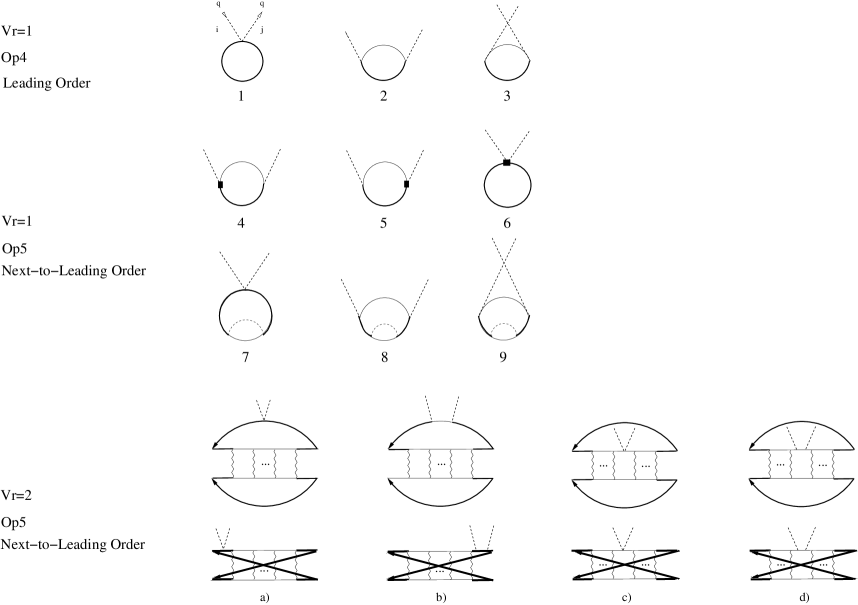
Figure 4: Contributions to the in-medium pion self-energy up to NLO or ${\cal O}(p^{5})$. The pions are indicated by the dashed lines and the squares correspond to NLO pion-nucleon vertices. The wiggly lines correspond to the nucleon-nucleon interaction kernel, see fig.5a, that is iterated as meant by the ellipsis.

3 Meson-baryon contributions to the pion self-energy

Let us apply the chiral counting given in eq.(2.11) to calculate the pion self-energy in the nuclear medium up to NLO or ${\cal O}(p^{5})$, with the different contributions shown in fig.4. The nucleon propagator, $G_{0}(k)_{i_{3}}$, contains both the free and the in-medium piece [46],

$$G_{0}(k)_{i_{3}}=\frac{\theta(\xi_{i_{3}}-|{\mathbf{k}}|)}{k^{0}-E({\mathbf{k}})-i\epsilon}+\frac{\theta(|{\mathbf{k}}|-\xi_{i_{3}})}{k^{0}-E({\mathbf{k}})+i\epsilon}=\frac{1}{k^{0}-E({\mathbf{k}})+i\epsilon}+i(2\pi)\theta(\xi_{i_{3}}-|{\mathbf{k}}|)\delta(k^{0}-E({\mathbf{k}}))~{}.$$ (3.1)

In this equation the subscript $i_{3}$ refers to the type of nucleon, so that, $i_{3}=p$  corresponds to the proton and $i_{3}=n$ to the neutron. Our convention for the pion self-energy, $\Sigma$, is such that the dressed pion propagator reads

$$\Delta_{\pi}(q)=\frac{1}{q^{2}-m_{\pi}^{2}+\Sigma}~{}.$$ (3.2)

We employ the pion-nucleon Heavy Baryon CHPT (HBCHPT) Lagrangians at ${\cal O}(p)$ and ${\cal O}(p^{2})$, that can be found e.g. in refs.[47, 48]. For completeness we reproduce them,

$${\cal L}_{\pi N}^{(1)} =\bar{N}(iD_{0}-\frac{g_{A}}{2}\vec{\sigma}\cdot\vec{u})N~{},$$

$${\cal L}_{\pi N}^{(2)} =\bar{N}\Biggl{(}\frac{1}{2M}\vec{D}\cdot\vec{D}+i\frac{g_{A}}{4M}\left\{\vec{\sigma}\cdot\vec{D},u_{0}\right\}+2c_{1}m_{\pi}^{2}(U+U^{\dagger})+\left(c_{2}-\frac{g_{A}^{2}}{8M}\right)u_{0}^{2}+c_{3}u_{\mu}u^{\mu}\Biggr{)}+\ldots$$ (3.3)

where the ellipses represent terms that are not needed here. In this equation, $N$ is the two component field of the nucleons, $g_{A}$ is the axial pion-nucleon coupling and $D_{\mu}=\partial_{\mu}+\Gamma_{\mu}$ the covariant chiral derivative, being $\Gamma_{\mu}=[u^{\dagger},\partial_{\mu}u]$. The pion fields $\vec{\pi}(x)$ enter in the matrix $u=\exp(i\vec{\tau}\cdot\vec{\pi}/2f)$, in terms of which $u_{\mu}=i\left\{u^{\dagger},\partial_{\mu}u\right\}$ and $U=u^{2}$, with $f$ the weak pion decay constant in the SU(2) chiral limit. The $c_{i}$ are chiral low energy constants whose values are fitted from phenomenology [48].

The leading contribution to the pion self-energy corresponds to the diagrams 1–3 on fig.4. The diagram 1 results by closing the Weinberg-Tomozawa pion-nucleon interaction (WT), obtained by expanding ${\cal L}_{\pi N}^{(1)}$ in eq.(3.3) up to two pion fields,

$$\Sigma_{1} =\frac{-iq^{0}}{2f^{2}}\varepsilon_{ij3}(\rho_{p}-\rho_{n})~{},$$ (3.4)

where the proton(neutron) density is given by $\rho_{p(n)}=\xi_{p(n)}^{3}/3\pi^{2}.$ $\Sigma_{1}$ is then a S-wave isovector self-energy. The sum of the diagrams 2 and 3 of fig.4 is

$$\Sigma_{2} =\frac{ig_{A}^{2}\,{\mathbf{q}}^{2}}{2f^{2}q^{0}}\varepsilon_{ij3}(\rho_{p}-\rho_{n})-\frac{g_{A}^{2}}{4f^{2}}\frac{({\mathbf{q}}^{2})^{2}}{mq_{0}^{2}}\delta_{ij}(\rho_{p}+\rho_{n})~{}.$$ (3.5)

They involve the one-pion vertex from ${\cal L}_{\pi N}^{(1)}$, which is proportional to $g_{A}$. This is a P-wave self-energy where the first term is isovector and the second is isoscalar.

Now, we move to the NLO contributions. The vertices from ${\cal L}_{\pi N}^{(2)}$ in eq.(3.3) are indicated by squares in the fig.4. It should be understood that the pion lines can leave or enter the diagrams 4 and 5 of fig.4. The sum of these two diagrams gives the result,

$$\Sigma_{3}=\frac{g_{A}^{2}{\mathbf{q}}^{2}}{2mf^{2}}(\rho_{p}+\rho_{n})\delta_{ij}~{}.$$ (3.6)

This is a P-wave isoscalar contribution that stems from the term linear in $g_{A}$ in ${\cal L}_{\pi N}^{(2)}$, that is a recoil correction to ${\cal L}_{\pi N}^{(1)}$. The diagram 6 of fig.4 is given by

$$\Sigma_{4}=\frac{-2\delta_{ij}}{f^{2}}\left(2c_{1}\,m_{\pi}^{2}-q_{0}^{2}(c_{2}+c_{3}-\frac{g_{A}^{2}}{8m})+c_{3}\,{\mathbf{q}}^{2}\right)(\rho_{p}+\rho_{n})~{},$$ (3.7)

in terms of the $c_{i}$ couplings of ${\cal L}_{\pi N}^{(2)}$, eq.(3.3). This is an isoscalar contribution where the term $-2\delta_{ij}c_{3}{\mathbf{q}}^{2}(\rho_{p}+\rho_{n})/f^{2}$ is P-wave and the rest is S-wave.

Next, let us consider the contributions to the pion self-energy due to the nucleon self-energy from a one-pion loop as depicted in the diagrams 7–9 of fig.4, with vertices calculated from ${\cal L}_{\pi N}^{(1)}$. The diagrams originate by dressing the in-medium nucleon propagator of the diagrams 1–3 by the one-pion loop nucleon self-energy,

$$\Sigma^{\pi}=\frac{1+\tau_{3}}{2}\Sigma_{p}^{\pi}+\frac{1-\tau_{3}}{2}\Sigma_{n}^{\pi}~{},$$ (3.8)

with $\Sigma_{p}^{\pi}$ and $\Sigma_{n}^{\pi}$ the proton and nucleon self-energies due to the in-medium pion-nucleon loop. Their values at $k^{0}=0$ are subtracted because we employ the physical nucleon mass. The contribution from the diagram 7 of fig.4 can be written as

$$\Sigma_{5} =\frac{q^{0}}{f^{2}}\varepsilon_{ij3}\int\frac{d^{4}k}{(2\pi)^{4}}\left(G_{0}(k)^{2}_{p}\Sigma_{p}^{\pi}-G_{0}(k)^{2}_{n}\Sigma_{n}^{\pi}\right)e^{ik^{0}\eta}~{},$$ (3.9)

where $e^{ik^{0}\eta}$, $\eta\to 0^{+}$, is the convergence factor associated to any closed loop made up by a single nucleon line [46]. Taking into account that

$$G_{0}(k)^{2}_{i_{3}}=-\partial G_{0}(k)_{i_{3}}/\partial k^{0}~{},$$ (3.10)

we then integrate by parts, which is possible thanks to the convergence factor. It results,

$$\Sigma_{5}=\frac{q^{0}}{f^{2}}\varepsilon_{ij3}\int\frac{d^{4}k}{(2\pi)^{4}}\left(G_{0}(k)_{p}\frac{\partial\Sigma_{p}^{\pi}}{\partial k^{0}}-G_{0}(k)_{n}\frac{\partial\Sigma_{n}^{\pi}}{\partial k^{0}}\right)e^{ik^{0}\eta}~{}.$$ (3.11)

Since $\eta\to 0$ the additional term obtained by taking the derivative of $e^{ik^{0}\eta}$ with respect to $k^{0}$ in eq.(3.9) does not contribute and is not shown. $\Sigma_{5}$ is an isovector S-wave pion self-energy contribution. For the diagrams 8 and 9 of the same figure one has analogously

$$\Sigma_{6} =-\frac{g_{A}^{2}}{f^{2}}\frac{{\mathbf{q}}^{2}}{q^{0}}\varepsilon_{ij3}\int\frac{d^{4}k}{(2\pi)^{4}}\left(G_{0}(k)_{p}\frac{\partial\Sigma^{\pi}_{p}}{\partial k^{0}}-G_{0}(k)_{n}\frac{\partial\Sigma^{\pi}_{n}}{\partial k^{0}}\right)e^{ik^{0}\eta}$$

$$+\frac{ig_{A}^{2}}{f^{2}}\frac{{\mathbf{q}}^{2}}{q_{0}^{2}}\delta_{ij}\int\frac{d^{4}k}{(2\pi)^{4}}\left(\ G_{0}(k)_{p}\Sigma^{\pi}_{p}+G_{0}(k)_{n}\Sigma^{\pi}_{n}\right)e^{ik^{0}\eta}~{}.$$ (3.12)

$\Sigma_{6}$ is a P-wave self-energy contribution but while the first line is of isovector character, the one in the second line is isoscalar. This last term is indeed a NNLO or ${\cal O}(p^{6})$ contribution because the pion-loop nucleon self-energy is ${\cal O}(p^{3})$ and we neglect it. The free pion-loop nucleon self-energy is calculated in HBCHPT [48], employing dimensional regularization in the $\overline{MS}-1$ scheme. Its derivative is

$$\frac{\partial\Sigma_{p(n),f}^{\pi}}{\partial k^{0}}=\frac{3g_{A}^{2}}{32\pi^{2}f^{2}}\left[m_{\pi}^{2}+k_{0}^{2}-3k^{0}\sqrt{b}\left(i\log\frac{k^{0}+i\sqrt{b}}{-k^{0}+i\sqrt{b}}+\pi\right)\right]~{},$$ (3.13)

with $b=m_{\pi}^{2}-k_{0}^{2}-i\eta~{}.$ Hence, because $\partial\Sigma_{p(n),f}^{\pi}/\partial k^{0}={\cal O}(p^{2})$ when inserted in $\Sigma_{5}$ and $\Sigma_{6}$ it gives rise to an ${\cal O}(p^{6})$ contribution that we neglect in the present work. The in-medium contribution to the pion-loop nucleon self-energy involves the finite integral

$$I_{m}=2\pi\int\frac{d^{4}\ell}{(2\pi)^{4}}\frac{{{\vec{\ell}}}^{2}\delta(k^{0}-\ell^{0})\theta(\xi_{i_{3}}-|{\mathbf{k}}-{\vec{\ell}}|)}{\ell^{2}-m_{\pi}^{2}+i\epsilon}=-\int\frac{d^{3}\ell}{(2\pi)^{3}}\frac{{{\vec{\ell}}}^{2}\theta(\xi_{i_{3}}-|{\mathbf{k}}-{\vec{\ell}}|)}{b+{\vec{\ell}}^{2}-i\epsilon}~{}.$$ (3.14)

This integral only depends on $k^{0}$ through the variable $b=m_{\pi}^{2}-k_{0}^{2}$. Since $\partial I_{m}/\partial k^{0}=-2k^{0}\partial I_{m}/\partial b={\cal O}(p^{2})$, because $k^{0}={\cal O}(p)$, the in-medium part of the pion loop contribution to the nucleon self-energy gives rise to ${\cal O}(p^{6})$ terms for the pion self-energy. As a result, $\Sigma_{5}$ and $\Sigma_{6}$ are at least ${\cal O}(p^{6})$. Notice that from eq.(2.10) these contributions were firstly booked as ${\cal O}(p^{5})$ because it was considered that $\partial\Sigma^{\pi}/\partial k^{0}={\cal O}(p)$ as $\Sigma^{\pi}={\cal O}(p^{3})$ and $k^{0}={\cal O}(p^{2})$. But since for these diagrams $V_{\rho}=1$, with only one closing nucleon line, $k^{0}={\cal O}(p)$.

4 In-medium nucleon-nucleon scattering contributions

We now consider those NLO contributions to the pion self-energy in the nuclear medium that involve the nucleon-nucleon interactions. They are depicted in the diagrams of the last two rows of fig.4, where the ellipsis indicate the iteration of the two-nucleon reducible loops. For the diagrams b) and d) of fig.4 the pion lines can leave or enter the diagrams. It is remarkable that these NLO contributions cancel between each other. On the other hand, since $V_{\rho}=2$ in these contributions one needs only the nucleon-nucleon scattering amplitude at ${\cal O}(p^{0})$ to match with our required precision at NLO. This amplitude is obtained by iterating in an infinite ladder of two nucleon reducible loops, with full in-medium nucleon propagators, the tree level amplitudes obtained from the ${\cal O}(p^{0})$ Lagrangian with four nucleons [3] and from the one-pion exchange with the lowest order pion-nucleon coupling. This procedure would correspond in vacuum to the leading nucleon-nucleon scattering amplitude according to refs.[2, 3].

Figure 5: a) The wiggly line represents the sum of the leading one-pion exchange and four-nucleon contact interactions, $T_{NN}^{c}+T_{NN}^{1\pi}$, eqs.(4.2) and (4.3). b) In-medium nucleon self-energy due to the nucleon-nucleon interactions with the Fermi seas.

The ${\cal O}(p^{0})$ lowest order four nucleon Lagrangian [3] is

$${\cal L}_{NN}^{(0)}=-\frac{1}{2}C_{S}(\overline{N}N)(\overline{N}N)-\frac{1}{2}C_{T}(\overline{N}\vec{\sigma}N)(\overline{N}\vec{\sigma}N)~{}.$$ (4.1)

Of course, this Lagrangian only contributes to the S-wave nucleon-nucleon scattering. The scattering amplitude for the process $N_{s_{1},i_{1}}({\mathbf{p}}_{1})N_{s_{2},i_{2}}({\mathbf{p}}_{2})\to N_{s_{3},i_{3}}({\mathbf{p}}_{3})N_{s_{4},i_{4}}({\mathbf{p}}_{4})$, with $s_{m}$ a spin label and $i_{m}$ an isospin one, that follows from the previous Lagrangian is

$$T_{NN}^{c} =-C_{S}\left(\delta_{s_{3}s_{1}}\delta_{s_{4}s_{2}}\,\delta_{i_{3}i_{1}}\delta_{i_{4}i_{2}}-\delta_{s_{3}s_{2}}\delta_{s_{4}s_{1}}\,\delta_{i_{3}i_{2}}\delta_{i_{4}i_{1}}\right)$$

$$-C_{T}\left(\vec{\sigma}_{s_{3}s_{1}}\cdot\vec{\sigma}_{s_{4}s_{2}}\,\delta_{i_{3}i_{1}}\delta_{i_{4}i_{2}}-\vec{\sigma}_{s_{3}s_{2}}\cdot\vec{\sigma}_{s_{4}s_{1}}\,\delta_{i_{3}i_{2}}\delta_{i_{4}i_{1}}\right)~{}.$$ (4.2)

Regarding the one-pion exchange at leading order, with vertices from ${\cal L}_{\pi N}^{(1)}$, one has the expression

$$T_{NN}^{1\pi}=\frac{g_{A}^{2}}{4f^{2}}\left[\frac{(\vec{\tau}_{i_{3}i_{1}}\cdot\vec{\tau}_{i_{4}i_{2}})(\vec{\sigma}\cdot{\mathbf{q}})_{s_{3}s_{1}}(\vec{\sigma}\cdot{\mathbf{q}})_{s_{4}s_{2}}}{{\mathbf{q}}^{2}+m_{\pi}^{2}-i\epsilon}\right.-\left.\frac{(\vec{\tau}_{i_{4}i_{1}}\cdot\vec{\tau}_{i_{3}i_{2}})(\vec{\sigma}\cdot{\mathbf{q}}^{\prime})_{s_{4}s_{1}}(\vec{\sigma}\cdot{\mathbf{q}}^{\prime})_{s_{3}s_{2}}}{{{\mathbf{q}}^{\prime}}^{2}+m_{\pi}^{2}-i\epsilon}\right]~{},$$ (4.3)

with ${\mathbf{q}}={\mathbf{p}}_{3}-{\mathbf{p}}_{1}$ and ${\mathbf{q}}^{\prime}={\mathbf{p}}_{4}-{\mathbf{p}}_{1}$. In the following, the sum $T_{NN}^{c}+T_{NN}^{1\pi}$ is represented diagrammatically by the exchange of a wiggly line, as in fig.5a.

The diagrams a) and c) of fig.4 involve the WT vertex while b) and d) contain the pole terms of pion-nucleon scattering. At leading order in the chiral counting the sum of the latter two has the same structure as the WT term, with the resulting vertex given by

$$-\frac{iq^{0}}{2f^{2}}\left(1-g_{A}^{2}\frac{{\mathbf{q}}^{2}}{q_{0}^{2}}\right)\varepsilon_{ijk}\tau^{k}~{}.$$ (4.4)

We can then discuss simultaneously all the diagrams in the last two rows of fig.4 employing the latter vertex. The sum of the diagrams a) and b) of fig.4 can be written in terms of the nucleon self-energy in the nuclear medium due to the nucleon-nucleon scattering. It reads

$$\Sigma_{7} =\frac{q^{0}}{2f^{2}}\left(1-g_{A}^{2}\frac{{\mathbf{q}}^{2}}{q_{0}^{2}}\right)\varepsilon_{ijk}\int\frac{d^{4}k_{1}}{(2\pi)^{4}}e^{ik_{1}^{0}\eta}\hbox{ Tr}\left\{\tau^{k}\left(\frac{1+\tau_{3}}{2}G_{0}(k_{1})_{p}+\frac{1-\tau_{3}}{2}G_{0}(k_{1})_{n}\right)\Sigma_{NN}\left(\frac{1+\tau_{3}}{2}G_{0}(k_{2})_{p}\right.\right.$$

$$\left.\left.+\frac{1-\tau_{3}}{2}G_{0}(k_{2})_{n}\right)\right\}~{}.$$ (4.5)

Here,

$$\Sigma_{NN}=\frac{1+\tau_{3}}{2}\Sigma_{p,NN}+\frac{1-\tau_{3}}{2}\Sigma_{n,NN}~{},$$ (4.6)

with $\Sigma_{p(n),NN}$ the proton (neutron) self-energy in the nuclear medium due to the nucleon-nucleon interactions, fig.5b,

$$\Sigma_{i_{3},NN}=-i\sum_{\alpha_{2},\sigma_{2}}\int\frac{d^{4}k_{2}}{(2\pi)^{4}}G_{0}(k_{2})_{\alpha_{2}}T_{NN}(k_{1}\sigma_{1}i_{3},k_{2}\sigma_{2}\alpha_{2}|k_{1}\sigma_{1}i_{3},k_{2}\sigma_{2}\alpha_{2})e^{ik_{2}^{0}\eta}~{}.$$ (4.7)

In this expression $T_{NN}$ is the nucleon-nucleon scattering amplitude between the indicated initial and final off-shell states. These are characterized by three labels. The first label corresponds to the four-momentum, the second to the spin and the third to the isospin. Note that in the equation there is a sum over all the quantum numbers of the second nucleon.

Proceeding similarly as before for $\Sigma_{5}$, including the integration by parts, we can write

$$\Sigma_{7} =\frac{q^{0}}{2f^{2}}\left(1-g_{A}^{2}\frac{{\mathbf{q}}^{2}}{q_{0}^{2}}\right)\varepsilon_{ij3}\sum_{\sigma_{1}}\int\frac{d^{4}k_{1}}{(2\pi)^{4}}\left(G_{0}(k_{1})_{p}\frac{\partial\Sigma_{p,NN}}{dk_{1}^{0}}-G_{0}(k_{1})_{n}\frac{\partial\Sigma_{n,NN}}{dk_{1}^{0}}\right)e^{ik_{1}^{0}\eta}~{}.$$ (4.8)

Inserting in the previous equation the explicit expression for $\Sigma_{i_{3},NN}$ of eq.(4.7) one has

$$\Sigma_{7} =-\frac{iq^{0}}{2f^{2}}\left(1-g_{A}^{2}\frac{{\mathbf{q}}^{2}}{q_{0}^{2}}\right)\varepsilon_{ij3}\sum_{\sigma_{1},\sigma_{2}}\int\frac{d^{4}k_{1}}{(2\pi)^{4}}\frac{d^{4}k_{2}}{(2\pi)^{4}}e^{ik_{1}^{0}\eta}e^{ik_{2}^{0}\eta}$$

$$\times\Biggl{[}G_{0}(k_{1})_{p}G_{0}(k_{2})_{p}\frac{\partial}{\partial k_{1}^{0}}T_{NN}(k_{1}\sigma_{1}p,k_{2}\sigma_{2}p|k_{1}\sigma_{1}p,k_{2}\sigma_{2}p)$$

$$-G_{0}(k_{1})_{n}G_{0}(k_{2})_{n}\frac{\partial}{\partial k_{1}^{0}}T_{NN}(k_{1}\sigma_{1}n,k_{2}\sigma_{2}n|k_{1}\sigma_{1}n,k_{2}\sigma_{2}n)\Biggr{]}~{}.$$ (4.9)

This result is obtained from eq.(4.8) by noting that

$$\sum_{\sigma_{1},\sigma_{2}}\int\frac{d^{4}k_{1}}{(2\pi)^{4}}\frac{d^{4}k_{2}}{(2\pi)^{4}}e^{ik_{1}^{0}\eta}e^{ik_{2}^{0}\eta} \Biggl{[}G_{0}(k_{1})_{p}G_{0}(k_{2})_{n}\frac{\partial}{\partial k_{1}^{0}}T_{NN}(k_{1}\sigma_{1}p,k_{2}\sigma_{2}n|k_{1}\sigma_{1}p,k_{2}\sigma_{2}n)$$

$$-G_{0}(k_{1})_{n}G_{0}(k_{2})_{p}\frac{\partial}{\partial k_{1}^{0}}T_{NN}(k_{1}\sigma_{1}n,k_{2}\sigma_{2}p|k_{1}\sigma_{1}n,k_{2}\sigma_{2}p)\Biggr{]}=0~{}.$$ (4.10)

This follows for two reasons. First, let us notice that because of Fermi-Dirac statistics

$$T_{NN}(k_{1}\sigma_{1}p,k_{2}\sigma_{2}n|k_{1}\sigma_{1}p,k_{2}\sigma_{2}n)=T_{NN}(k_{2}\sigma_{2}n,k_{1}\sigma_{1}p|k_{2}\sigma_{2}n,k_{1}\sigma_{1}p)~{}.$$ (4.11)

Second, at LO the amplitude $T_{NN}$, as commented above, is given by the iteration of the wiggly line in fig.5. The latter does neither depend on $k_{1}^{0}$ nor on $k_{2}^{0}$, see eqs.(4.2) and (4.3). Since the two-nucleon reducible unitarity loop, the one in fig.6b, depends on $k_{1}^{0}$ and $k_{2}^{0}$ through their sum, $k_{1}^{0}+k_{2}^{0}$, as can be seen straightforwardly [49], it results that $T_{NN}$ at LO only depends on them in this way. It follows then that $\partial T_{NN}/\partial k_{1}^{0}=\partial T_{NN}/\partial k_{2}^{0}$. Taking these two facts into account, as $k_{i}$ and $\sigma_{i}$ are dummy variables, eq.(4.10) results.

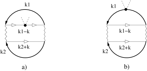
Figure 6: Contribution to the pion self-energy with a two-nucleon reducible loop. The pion scatters inside/outside the loop for the diagram a)/b).

Let us now consider the diagrams c) and d) of fig.4 whose contribution is denoted by $\Sigma_{8}$. These diagrams consist of the pion-nucleon scattering in a two-nucleon reducible loop which is corrected by initial and final state interactions. The iterations are indicated by the ellipsis on both sides of the diagrams. In order to see that these diagrams cancel with eq.(4.9) let us take first the diagram of fig.6a with a twice iterated wiggly line vertex. It is given by

$$\Sigma_{8}^{L} =i\frac{q^{0}}{2f^{2}}\left(1-g_{A}^{2}\frac{{\mathbf{q}}^{2}}{q_{0}^{2}}\right)\varepsilon_{ij3}\sum_{\alpha,\beta}\sum_{\sigma_{1},\sigma_{2}}\int\frac{d^{4}k_{1}}{(2\pi)^{4}}\frac{d^{4}k_{2}}{(2\pi)^{4}}G_{0}(k_{1})_{\alpha}G_{0}(k_{2})_{\beta}e^{ik_{1}^{0}\eta}e^{ik_{2}^{0}\eta}$$

$$\times\Biggl{[}\frac{-i}{2}\int\frac{d^{4}q}{(2\pi)^{4}}\sum_{\alpha^{\prime},\beta^{\prime}}\sum_{\sigma^{\prime}_{1},\sigma^{\prime}_{2}}V_{\alpha\beta;\alpha^{\prime}\beta^{\prime}}(q)\frac{\partial G_{0}(k_{1}-q)_{\alpha^{\prime}}}{\partial k_{1}^{0}}\left.\tau_{3}\right|_{\alpha^{\prime}\alpha^{\prime}}V_{\alpha^{\prime}\beta^{\prime};\alpha\beta}(-q)G_{0}(k_{2}+q)_{\beta^{\prime}}\Biggr{]}~{},$$ (4.12)

where $V_{\alpha\beta;\gamma\delta}$ corresponds to the wiggly line with the indices $\alpha$ and $\gamma$ belonging to the out-/in-going first particle, in that order, and similarly $\beta$ and $\delta$ for the second one. To shorten the notation, we have only indicated the isospin indices in $V$ in the previous equation, although $V$ depends also on spin. A symmetry factor $1/2$ is also included because $V_{\alpha\beta;\gamma\delta}$ contains both the direct and exchange terms, as explicitly shown in eqs.(4.2) and (4.3). The derivative with respect to $k_{1}^{0}$ arises in eq.(4.12) because the nucleon propagator to which the two pions are attached appears squared and we have made use of eq.(3.10). This is so because for the $\pi^{\pm}$, $i$ and $j$ can be either 1 or 2, so that the only surviving contribution is $k=3$. For the $\pi^{0}$, $i=j=3$ and then there is no contribution. Thus, because one has either 0 or $\tau^{3}$, which is a diagonal matrix, the nucleon propagator before and after the two-pion vertex is the same. The $q$-loop integral in eq.(4.12) is typically divergent. Nevertheless, the parametric derivative with respect to $k_{1}^{0}$ can be extracted out of the integral as soon as it is regularized. Of course, the same regularization method as that used to calculate $T_{NN}$ should be employed. Once the derivative is taken out of the integral, the quantity between the squared brackets in eq.(4.12) corresponds to the twice iterated wiggly line contribution to $T_{NN}(k_{1}\sigma_{1}\alpha,k_{2}\sigma_{2}\beta|k_{1}\sigma_{1}\alpha,k_{2}\sigma_{2}\beta)$. In addition, the isovector nature of the modified WT vertex of eq.(4.4) implies that only the difference between the proton-proton and neutron-neutron contributions arises. This can be worked out straightforwardly from the isospin structure of the local four-nucleon vertex and that of the one-pion exchange [49]. As a result we can write

$$\Sigma_{8}^{L} =\frac{iq^{0}}{2f^{2}}\left(1-g_{A}^{2}\frac{{\mathbf{q}}^{2}}{q_{0}^{2}}\right)\varepsilon_{ij3}\sum_{\sigma_{1},\sigma_{2}}\int\frac{d^{4}k_{1}}{(2\pi)^{4}}\frac{d^{4}k_{2}}{(2\pi)^{4}}\Biggr{[}G_{0}(k_{1})_{p}G_{0}(k_{2})_{p}\frac{\partial}{\partial k_{1}^{0}}T_{NN}^{L}(k_{1}\sigma_{1}p,k_{2}\sigma_{2}p|k_{1}\sigma_{1}p,k_{2}\sigma_{2}p)$$

$$-G_{0}(k_{1})_{n}G_{0}(k_{2})_{n}\frac{\partial}{\partial k_{1}^{0}}T_{NN}^{L}(k_{1}\sigma_{1}n,k_{2}\sigma_{2}n|k_{1}\sigma_{1}n,k_{2}\sigma_{2}n)\Biggl{]}e^{ik_{1}^{0}\eta}e^{ik_{2}^{0}\eta}~{},$$ (4.13)

where the superscript $L$ on top of $T_{NN}$ indicates that this scattering amplitude is calculated at the one-loop level. This result then cancels exactly with that of fig.6b, corresponding to the twice iterated wiggly line exchange contribution to $T_{NN}$ in eq.(4.9). This cancellation is explicit by reducing eq.(4.9) to the one-loop case for calculating $T_{NN}$. Notice as well that the contribution to $T_{NN}$ given by the exchange of only one wiggly line vanishes when inserted in eq.(4.9) because it is independent of $k_{1}^{0}$, see eqs.(4.2) and (4.3).

This process of mutual cancellation between $\Sigma_{7}$ and $\Sigma_{8}$ can be generalized to any number of two-nucleon reducible loops in figs.4a), b) and 4c) and d), respectively. An $n+1$ iterated wiggly line exchange in these figures implies $n$ two-nucleon reducible loops. The two pions can be attached for $\Sigma_{8}$ to any of them, while for $\Sigma_{7}$ the derivative with respect to $k_{1}^{0}$ can also act on any of the loops. The iterative loops are the same for both cases but a relative minus sign results from the loop on which the two pions are attached with respect to the one on which the derivative is acting, as just discussed. This is exemplified in fig.7 for the case with two two-nucleon reducible loops. Hence,

$$\Sigma_{7}+\Sigma_{8}=0~{}.$$ (4.14)

The basic simple reason for such cancellation is that while for $\Sigma_{7}$ the presence of a nucleon propagator squared gives rise to $(-1)^{2}\partial/\partial k_{1}^{0}$, for $\Sigma_{8}$ it yields $-\partial/\partial k_{1}^{0}$, cf. eqs.(4.9) and (4.12), respectively. The extra $(-1)$ for $\Sigma_{7}$ results because it involves an integration by parts, as discussed above.

Figure 7: In this figure the cross indicates the action of the derivative with respect to $k_{1}^{0}$ in eq.(4.9). When the derivative is performed over a baryon propagator the latter becomes squared, according to eq.(3.10). In this way, the first diagram on the second row of the figure is the same as the one to the left of the first row but with opposite sign and they cancel each other. The same applies to the second diagrams on the first and second rows.

5 Conclusions and outlook

We have developed a promising scheme for an EFT in the nuclear medium that combines both short-range and pion-mediated inter-nucleon interactions. It is based on the development of a new chiral power counting which is bounded from below and at a given order it requires to calculate a finite number of contributions. The latter could eventually involve infinite strings of two–nucleon reducible diagrams with the leading ${\cal O}(p^{0})$ two-nucleon CHPT amplitudes. As a result, our power counting accounts for non-perturbative effects to be resummed which, e.g., give rise to the generation of the deuteron in vacuum nucleon-nucleon scattering. The power counting from the onset takes into account the presence of enhanced nucleon propagators and it can also be applied to multi-nucleon forces.

We have then calculated the leading corrections to the lowest order result for the pion self-energy in asymmetric nuclear matter, with all the contributions up-to-and-including ${\cal O}(p^{5})$ evaluated. As a novelty, it is shown that the leading corrections to the linear density approximation vanish. In particular, it is derived that the leading corrections from nucleon-nucleon scattering mutually cancel. This suppression is interesting since it allows to understand from first principles the phenomenological success of fitting data on pionic atoms with only meson-baryon interactions [37, 33]. An ${\cal O}(p^{6})$ calculation of the pion self-energy is a very interesting task as it provides the first corrections to the linear density approximation, e.g. the well-known Ericson-Ericson-Pauli rescattering effect [32]. More calculations for other physical processes and higher orders are clearly needed to assess the realm of applicability of the present approach.

References

- [1] S. Weinberg, Physica A 96 (1979) 327.
- [2] S. Weinberg, Phys. Lett. B 251 (1990) 288.
- [3] S. Weinberg, Nucl. Phys. B 363 (1991) 3.
- [4] C. Ordonez, L. Ray and U. van Kolck, Phys. Rev. C 53 (1996) 2086.
- [5] U. van Kolck, Prog. Part. Nucl. Phys. 43 (1999) 337.
- [6] D. R. Entem and R. Machleidt, Phys. Rev. C 68 (2003) 041001.
- [7] E. Epelbaum, W. Glöckle and U.-G. Meißner, Nucl. Phys. A 671 (2000) 295; Nucl. Phys. A 747 (2005) 362.
- [8] E. Epelbaum, H. Kamada, A. Nogga, H. Witala, W. Glöckle and U.-G. Meißner, Phys. Rev. Lett. 86 (2001) 4787.
- [9] E. Epelbaum, Prog. Part. Nucl. Phys. 57 (2006) 654.
- [10] E. Epelbaum, H. W. Hammer and U.-G. Meißner, Rev. Mod. Phys., to appear, arXiv:0811.1338 [nucl-th].
- [11] R. J. Furnstahl, G. Rupak and T. Schäfer, Ann. Rev. Part. Nucl. Sci. 58 (2008) 1.
- [12] S. K. Bogner, R. J. Furnstahl, S. Ramanan and A. Schwenk, Nucl. Phys. A 773 (2006) 203; S. K. Bogner, A. Schwenk, R. J. Furnstahl and A. Nogga, Nucl. Phys. A 763 (2005) 59.
- [13] N. Kaiser, M. Mühlbauer and W. Weise, Eur. Phys. J. A 31 (2007) 53.
- [14] P. Saviankou, S. Krewald, E. Epelbaum and U.-G. Meißner, arXiv:0802.3782 [nucl-th].
- [15] P. Navratil, V. G. Gueorguiev, J. P. Vary, W. E. Ormand and A. Nogga, Phys. Rev. Lett. 99 (2007) 042501.
- [16] J. A. Oller, Phys. Rev. C 65 (2002) 025204.
- [17] U.-G. Meißner, J. A. Oller and A. Wirzba, Annals Phys. 297 (2002) 27.
- [18] L. Girlanda, A. Rusetsky and W. Weise, Annals Phys. 312 (2004) 92.
- [19] N. Kaiser, S. Fritsch and W. Weise, Nucl. Phys. A 697 (2002) 255.
- [20] N. Kaiser, S. Fritsch and W. Weise, Nucl. Phys. A 724 (2003) 47.
- [21] S. Fritsch, N. Kaiser and W. Weise, Nucl. Phys. A 750 (2005) 259.
- [22] R. Rockmore, Phys. Rev. C 40 (1989) 13.
- [23] M. Döring and E. Oset, Phys. Rev. C 77 (2008) 024602.
- [24] E. Oset, C. Garcia-Recio and J. Nieves, Nucl. Phys. A 584 (1995) 653.
- [25] T. S. Park, H. Jung and D. P. Min, J. Korean Phys. Soc. 41 (2002) 195.
- [26] J. Goldstone, A. Salam and S. Weinberg, Phys. Rev. 127 (1962) 965.
- [27] J. Gasser and H. Leutwyler, Annals Phys. 158 (1984) 142; Nucl. Phys. B 250 (1985) 465.
- [28] N. H. Fuchs, H. Sazdjian and J. Stern, Phys. Lett. B 269 (1991) 183; Phys. Rev. D 47 (1993) 3814.
- [29] G. Colangelo, J. Gasser and H. Leutwyler, Phys. Rev. Lett. 86 (2001) 5008.
- [30] V. Thorsson and A. Wirzba, Nucl. Phys. A 589 (1995) 633; ”Hirschegg ’95: Dynamical Properties of Hadrons in Nuclear Matter” (H. Feldmeier and W.Nörenberg, Eds.), pp. 31-43, GSI-print, Darmstadt, 1995; M. Kirchbach and A. Wirzba, Nucl. Phys. A 604 (1996) 395; ibid A 616 (1997) 648.
- [31] N. Kaiser and W. Weise, Phys. Lett. B 671 (2009) 25.
- [32] M. Ericson and T. E. O. Ericson, Annals Phys. 36 (1966) 323.
- [33] E. Friedman and A. Gal, Phys. Rept. 452 (2007) 89, and references therein.
- [34] G. Chanfray, M. Ericson and M. Oertel, Phys. Lett. B 563 (2003) 61.
- [35] N. Kaiser and W. Weise, Phys. Lett. B 512 (2001) 283.
- [36] L. Girlanda, A. Rusetsky and W. Weise, Nucl. Phys. A 755 (2005) 653.
- [37] E. E. Kolomeitsev, N. Kaiser and W. Weise, Phys. Rev. Lett. 90 (2003) 092501.
- [38] J. D. Walecka, Annals Phys. 83 (1974) 491.
- [39] B. D. Serot and J. D. Walecka, Adv. Nucl. Phys. 16 (1986) 1.
- [40] B. D. Serot, Rept. Prog. Phys. 55, 1855 (1992).
- [41] B. D. Serot and J. D. Walecka, arXiv:nucl-th/0010031.
- [42] R. J. Furnstahl and B. D. Serot, Comments Nucl. Part. Phys. 2 (2000) A23.
- [43] J. A. McNeil, J. R. Shepard and S. J. Wallace, Phys. Rev. Lett. 50 (1983) 1439; B. C. Clark, S. Hama, R. L. Mercer, L. Ray and B. d. Serot, Phys. Rev. Lett. 50 (1983) 1644.
- [44] J. Gasser, M. E. Sainio and A. Svarc, Nucl. Phys. B 307 (1988)779.
- [45] B. Borasoy, E. Epelbaum, H. Krebs, D. Lee and U.-G. Meißner, Eur. Phys. J. A 31 (2007) 105.
- [46] A. L. Fetter and J. D. Walecka, “Quantum Theory of Many-Particle Systems”. Dover Publications, Inc., Mineola, New York, 2003.
- [47] N. Kaiser, R. Brockmann and W. Weise, Nucl. Phys. A 625 (1997) 758
- [48] V. Bernard, N. Kaiser and U.-G. Meißner, Int. J. Mod. Phys. E 4 (1995) 193.
- [49] A. Lacour, J. A. Oller and U.-G. Meißner, “Non-perturbative methods for a chiral effective field theory of finite density nuclear systems,” arXiv:0906.2349 [nucl-th].