Mesoscopic Properties of
Molecular Folding and Aggregation Processes

Abstract

Protein folding, peptide aggregation and crystallization, as well as adsorption of molecules on soft or solid substrates have an essential feature in common: In all these processes, structure formation is guided by a collective, cooperative behavior of the molecular subunits lining up to build chainlike macromolecules. Proteins experience conformational transitions related to thermodynamic phase transitions. For chains of finite length, an important difference of crossovers between conformational (pseudo)phases is, however, that these transitions are typically rather smooth processes, i.e., thermodynamic activity is not necessarily signalized by strong entropic or energetic fluctuations. Nonetheless, in order to understand generic properties of molecular structure-formation processes, the analysis of mesoscopic models from a statistical physics point of view enables first insights into the nature of conformational transitions in small systems. Here, we review recent results obtained by means of sophisticated generalized-ensemble computer simulations of minimalistic coarse-grained models.

1 Introduction

At the atomic level, proteins have a complex chemical structure which is formed and stabilized by the electronic properties of the atoms. Thus, the precise analysis of structure and dynamical behavior of molecules require a detailed knowledge of the quantum mechanics involved. For molecular systems of interest, where even the smallest molecules contain hundreds to thousands of atoms, a quantum-mechanical analysis is usually simply impossible, a fortiori if effects of the environment (e.g., an aqueous solution) are non-negligible. This problem reflects the dilemma of “realistic” all-atom models which are based on semiclassical assumptions and, consequently, depend on hundreds of parameters mimicking quantum-mechanical effects. Actually, taken with sufficient care, the application of such models is often inevitable if specific questions on atomic scales shall be investigated.

However, from a physics point of view, one may ask: Is it really necessary at all to employ all-atom models, if one is interested in generic features of molecular mechanics which typically anyway requires a cooperative action of larger subunits (monomers)? The answer would be “no”, if conformational transitions accompanying molecular structure-formation processes indeed exhibit similarities to thermodynamic phase transitions, in which case it should be possible to reveal general, qualitative properties by analyses of suitably simplified models on mesoscopic scales shak1 ; bj1 .

After a few evolutionary remarks and introducing typical mesoscopic models, we eventually present results from studies of protein folding and peptide aggregation processes which lead to the conclusion that characteristic features of the identified conformational transitions are also relevant in corresponding natural structuring processes.

2 The evolutionary aspect

The number of different functional proteins encoded in the human DNA is of order 100 000 – an extremely small number compared to the total number of possibilities: Recalling that 20 amino acids line up natural proteins and typical proteins consist of $N\sim{\cal O}(10^{2}-10^{3})$ amino acid residues, the number of possible primary structures $20^{N}$ lies somewhere far, far above $\text{20}^{\text{100}}\sim\text{10}^{\text{130}}$. Assuming all proteins were of size $N=100$ and a single folding event would take 1 ms, a sequential enumeration process would need about $\text{10}^{\text{119}}$ years to generate structures of all sequences, irrespective of the decision about their “fitness”, i.e., the functionality and ability to efficiently cooperate with other proteins in a biological system. Of course, one might argue that the evolution is a highly parallelized process which drastically increases the generation rate. So, we can ask the question, how many processes can maximally run in parallel.

The universe contains of the order of $\text{10}^{\text{80}}$ protons. Assuming further that an average amino acid consists of at least 50 protons, a chain with $N=100$ amino acids has of the order ${\cal O}(10^{3})$ protons, i.e., $\text{10}^{\text{77}}$ sequences could be generated in each millisecond (forgetting for the moment that some proton-containing machinery is necessary for the generation process and only a small fraction of protons is assembled in earth-bound organic matter). The age of our universe is about $\text{10}^{\text{10}}$ years (we also forget that the Earth is even about one order of magnitude younger) or $\text{10}^{\text{21}}$ ms. Hence, about $\text{10}^{\text{98}}$ sequences could have been tested to date, if our drastic simplifications were right. But even this yet much too optimistic estimate is still noticeably smaller than the above mentioned reference number of $\text{10}^{\text{130}}$ possible sequences for a 100-mer.

At least two conclusions can be drawn from this crude analysis. One thing is that the evolutionary process of generating and selecting sequences is ongoing as it is likely that only a small fraction of functional proteins has been identified yet by nature. On the other hand, the existence of complex biological systems, where hundreds of thousands different types of macromolecules interact efficiently, can only be explained by means of efficient evolutionary strategies of adaptation to environmental conditions on Earth which dramatically changed through billions of years. Furthermore, the development from primitive to complex biological systems leads to the conclusion that within the evolutionary process of protein design, particular patterns in the genetic code have survived over generations, while others were improved (or deselected) by recombinations, selections, and mutations. But the sequence question is only one side. Another regards the geometric structures of proteins which are directly connected to biological functionalities. The conformational similarity among human functional proteins is also quite surprising; only of the order of 1 000 significantly different “folds” were identified tang1 .

Since the conformation space is infinitely large because of the continuous degrees of freedom and the sequence space is also giant, the protein folding problem is typically attacked from two sides: the direct folding problem, where the amino acid sequence is given and the associated native, functional conformation has to be identified, and the inverse folding problem, where one is interested in all sequences that fold into a given target conformation. With these two approaches, it is, however, virtually impossible to unravel evolutionary factors that led to the set of present functional proteins. Only for very simple protein models, a comprising statistical analysis of sequence and conformation spaces is possible.

3 Simple approaches to coarse-grained modeling of proteins

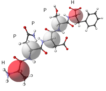
Figure 1: Coarse-graining peptides in a “united atom” approach. Each amino acid is contracted to a single “C^α” interaction point. The effective distance between adjacent, bonded interaction sites is about 3.8 Å. In the coarse-grained hydrophobic-polar models considered here, the interaction sites have no steric extension. The excluded volume is modeled via type-specific Lennard-Jones pair potentials. In hydrophobic-polar (HP) peptide models, only hydrophobic (H) and polar (P) amino acid residues are distinguished.

Coarse-graining of models, where relevant length scales are increased by reducing the number of microscopic degrees of freedom, has proven to be very successful in polymer science and protein folding bj1 . Although specificity is much more sensitive for proteins, since details (charges, polarity, etc.) and differences of the amino acid side chains can have strong influences on the fold, also here mesoscopic approaches are of essential importance for the basic understanding of conformational transitions affecting the folding process. It is also the only possible approach for systematic analyses of basic problems such as the evolutionarily significant question why only a few sequences in nature are “designing” and thus relevant for selective functions. On the other hand, what is the reason why proteins prefer a comparative small set of target structures, i.e., what explains the preference of designing sequences to fold into the same three-dimensional structure? Many of these questions are still widely unanswered yet. Actually, the complexity of these questions requires a huge number of comparative studies of complete classes of peptide sequences and structures that cannot be achieved by means of computer simulations of microscopic models. Currently only two approaches are promising. One is the bioinformatics approach of designing and scoring sequences and structures (and also possible combinations of receptors and ligands in aggregates), often based on data base scanning according to certain criteria. Another, more physically motivated approach makes use of coarse-grained models, where only a few specific properties of the monomers enter into the models. Since a characteristic feature of non-membrane proteins is to possess a compact hydrophobic core, screened from the surrounding solvent by a shell of polar monomers, frequently only two types of amino acids are distinguished: hydrophobic (H) and polar (P) residues, giving the class of corresponding models the name “hydrophobic-polar” (HP) models (see Fig. 1).

3.1 The HP model for lattice proteins

In the simplest case, the HP peptide chain is a linear, self-avoiding chain of H and P residues on a regular lattice tang1 ; dill1 . Such models allow a comprising analysis of both, the conformation and sequence space, e.g., by exactly enumerating all combinatorial possibilities schbj1 . Other important aspects in lattice model studies are the identification of lowest-energy conformations of comparatively long sequences and the characterization of the folding thermodynamics bj2 .

In the HP model, a monomer of an HP sequence $\bm{\sigma}=(\sigma_{1},\sigma_{2},\ldots,\sigma_{N})$ is characterized by its residual type ($\sigma_{i}=P$ for polar and $\sigma_{i}=H$ for hydrophobic residues), the position $1\leq i\leq N$ within the chain of length $N$, and the spatial position ${\bf x}_{i}$ to be measured in units of the lattice spacing. A conformation is then symbolized by the vector of the coordinates of successive monomers, ${\bf X}=({\bf x}_{1},{\bf x}_{2},\ldots,{\bf x}_{N})$. The distance between the $i$th and the $j$th monomer is denoted by $r_{ij}=|{\bf x}_{i}-{\bf x}_{j}|$. The bond length between adjacent monomers in the chain is identical with the spacing of the used regular lattice with coordination number $q$. These covalent bonds are thus not stretchable. A monomer and its nonbonded nearest neighbors may form so-called contacts. Therefore, the maximum number of contacts of a monomer within the chain is $(q-2)$ and $(q-1)$ for the monomers at the ends of the chain. To account for the excluded volume, lattice proteins are self-avoiding, i.e., two monomers cannot occupy the same lattice site. The total energy for an HP protein reads in energy units $\varepsilon_{0}$ (we set $\varepsilon_{0}=1$ in the following)

$$E_{\text{HP}}=\varepsilon_{0}\sum\limits_{\langle i,j>i+1\rangle}C_{ij}U_{\sigma_{i}\sigma_{j}},$$ (1)

where $C_{ij}=(1-\delta_{i+1\,j})\Delta(x_{ij}-1)$ with

$$\Delta(z)=\left\{\begin{array}[]{cl}1,&\hskip 8.53581ptz=0,\\ 0,&\hskip 8.53581ptz\neq 0\end{array}\right.$$ (2)

is a symmetric $N\times N$ matrix called contact map and

$$U_{\sigma_{i}\sigma_{j}}=\left(\begin{array}[]{cc}u_{HH}&u_{HP}\\ u_{HP}&u_{PP}\end{array}\right)$$ (3)

is the $2\times 2$ interaction matrix. Its elements $u_{\sigma_{i}\sigma_{j}}$ correspond to the energy of $HH$, $HP$, and $PP$ contacts. For labeling purposes we shall adopt the convention that $\sigma_{i}=0\,\hat{=}\,P$ and $\sigma_{i}=1\,\hat{=}\,H$.

In the simplest formulation dill1 , only the attractive hydrophobic interaction is nonzero, $u^{\text{HP}}_{HH}=-1,u^{\text{HP}}_{HP}=u^{\text{HP}}_{PP}=0$. Therefore, $U^{\text{HP}}_{\sigma_{i}\sigma_{j}}=-\delta_{\sigma_{i}H}\delta_{\sigma_{j}H}$. This parametrization has been extensively used to identify ground states of HP sequences, some of which are believed to show up qualitative properties comparable with realistic proteins whose 20-letter sequence was transcribed into the 2-letter code of the HP model dill3 ; unger1 ; shak2 ; 103lat ; 103toma .

This simple form of the standard HP model suffers, however, from the fact that the lowest-energy states are usually highly degenerate and therefore the number of designing sequences (i.e., sequences with unique ground state) is very small. Incorporating additional inter-residue interactions tang1 , symmetries are broken, degeneracies are smaller, and the number of designing sequences increases schbj1 .

3.2 A simple off-lattice generalization: The AB model

Since lattice models suffer from undesired effects of the underlying lattice symmetries, simple hydrophobic-polar off-lattice models were defined. One such model is the AB model, where, for historical reasons, A symbolizes hydrophobic and B polar regions of the protein, whose conformations are modeled by polymer chains in continuum space governed by effective bending energy and van der Waals interactions still1 . These models allow for the analysis of different mutated sequences with respect to their folding characteristics. Here, the idea is that the folding transition is a kind of pseudophase transition which can in principle be described by one or a few order-like parameters. Depending on the sequence, the folding process can be highly cooperative (downhill folding), less cooperative depending on the height of a free-energy barrier (two-state folding), or even frustrating due to the existence of different barriers in a metastable regime (crystal or glassy phases) baj1 ; ssbj1 . These characteristics known from functional proteins can be recovered in the AB model, which is computationally much less demanding than all-atom formulations and thus enables throughout theoretical analyses.

We denote the spatial position of the $i$th monomer in a heteropolymer consisting of $N$ residues by ${\bf x}_{i}$, $i=1,\ldots,N$, and the vector connecting nonadjacent monomers $i$ and $j$ by ${\bf r}_{ij}={\bf x}_{i}-{\bf x}_{j}$. For covalent bond vectors, we set $|{\bf b}_{i}|\equiv|{\bf r}_{i\,i+1}|=1$. The bending angle between monomers $k$, $k+1$, and $k+2$ is $\vartheta_{k}$ ($0\leq\vartheta_{k}\leq\pi$) and $\sigma_{i}=A,B$ symbolizes the type of the monomer. In the AB model still1 , the energy of a conformation is given by

$$E_{\text{AB}}=\frac{1}{4}\sum\limits_{k=1}^{N-2}(1-\cos\vartheta_{k})+4\sum\limits_{i=1}^{N-2}\sum\limits_{j=i+2}^{N}\left(\frac{1}{r_{ij}^{12}}-\frac{C(\sigma_{i},\sigma_{j})}{r_{ij}^{6}}\right),$$ (4)

where the first term is the bending energy and the sum runs over the $(N-2)$ bending angles of successive bond vectors. The second term partially competes with the bending barrier by a potential of Lennard-Jones type. It depends on the distance between monomers being nonadjacent along the chain and accounts for the influence of the AB sequence on the energy. The long-range behavior is attractive for pairs of like monomers and repulsive for $AB$ pairs of monomers:

$$C(\sigma_{i},\sigma_{j})=\left\{\begin{array}[]{cl}+1,&\hskip 19.91692pt\sigma_{i},\sigma_{j}=A,\\ +1/2,&\hskip 19.91692pt\sigma_{i},\sigma_{j}=B,\\ -1/2,&\hskip 19.91692pt\sigma_{i}\neq\sigma_{j}.\\ \end{array}\right.$$ (5)

The AB model is a C^α type model in that each residue is represented by a single interaction site only, the “C^α atom” (see Fig. 1). Thus, the natural dihedral torsional degrees of freedom of realistic protein backbones are replaced by virtual bond and torsion angles. The large torsional barrier of the peptide bond between neighboring amino acids is in the AB model effectively taken into account by introducing the bending energy.

Although this coarse-grained picture will obviously not be sufficient to reproduce microscopic properties of specific realistic proteins, it qualitatively exhibits, however, sequence-dependent features known from nature, as, for example, tertiary folding pathways characteristic for two-state folding, folding through intermediates, or metastability ssbj1 , and two-state kinetics kbj1 .

4 Thermodynamics of heteropolymer folding

For the analysis of conformational transitions accompanying the tertiary folding behavior of lattice proteins, multicanonical chain-growth simulations bj1 ; bj2 can be efficiently performed for the HP model. An example is the 42-mer with the sequence $PH_{2}PHP$$H_{2}$$P$$H$$P$$H$$P_{2}$$H_{3}$$P$$H$$P$$H_{2}$$P$$H$$P$$H_{3}$$P_{2}$$H$$P$$H$$P$$H_{2}$$P$$HPH_{2}P$ that forms a parallel helix in the ground state. Originally, it was designed to serve as a lattice model of the parallel $\beta$ helix of pectate lyase C yoder . But there are additional properties that make it an interesting and challenging system. The ground-state energy is known to be $E_{\text{min}}=-34$. In the simulations, the ground-state degeneracy was estimated to be $g_{0}=3.9\pm 0.4$ bj1 ; bj2 , which is in perfect agreement with the known value $g_{0}^{\text{ex}}=4$ (except translational, rotational, and reflection symmetries) dill4 . As we will see, there are two conformational transitions. At low temperatures, fluctuations of energetic and structural quantities signalize a (pseudo)transition between the lowest-energy states possessing compact hydrophobic cores and the regime of globular conformations, and at a higher temperature, there is another transition between globules and random coils.

The average structural properties at finite temperatures can be characterized best by the mean end-to-end distance $\langle R_{\text{ee}}\rangle(T)$ and the mean radius of gyration $\langle R_{\text{gyr}}\rangle(T)$. Multicanonical chain-growth simulation results for $\langle R_{\text{ee}}\rangle(T)$ and $\langle R_{\text{gyr}}\rangle(T)$ of the 42-mer are shown in Fig. 2.

Figure 2: Mean end-to-end distance $\langle R_{\text{ee}}\rangle$ and mean radius of gyration $\langle R_{\text{gyr}}\rangle$ of the 42-mer.

The pronounced minimum in the end-to-end distance can be interpreted as an indication of the transition between the lowest-energy states and globules: The small number of ground states have similar and highly symmetric shapes (due to the reflection symmetry of the sequence) but the ends of the chain are polar and therefore they are not required to reside close to each other. Increasing the temperature allows the protein to fold into conformations different from the ground states and contacts between the ends become more likely. Therefore, the mean end-to-end distance decreases and the protein has entered the globular “phase”. Further increasing the temperature leads then to a disentanglement of globular structures and random coil conformations with larger end-to-end distances dominate. In Fig. 3, we have plotted the specific heat $C_{V}(T)$ and the derivatives of the mean end-to-end distance and of the mean radius of gyration with respect to the temperature, $d\langle R_{\text{ee}}\rangle/dT$ and $d\langle R_{\text{gyr}}\rangle/dT$.

Two temperature regions of conformational activity (shaded in gray), where the curves of the fluctuating quantities exhibit extremal points, can clearly be separated. We estimate the temperature region of the ground-state – globule transition to be within $T_{0}^{(1)}\approx 0.24$ and $T_{0}^{(2)}\approx 0.28$. The globule – random coil transition takes place between $T_{1}^{(1)}\approx 0.53$ and $T_{1}^{(2)}\approx 0.70$.

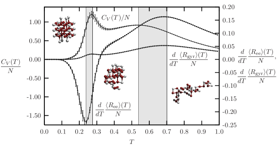
Figure 3: Specific heat $C_{V}$ and derivatives w.r.t. temperature of mean end-to-end distance $\langle R_{\text{ee}}\rangle$ and radius of gyration $\langle R_{\text{gyr}}\rangle$ as functions of temperature for the 42-mer. The ground-state – globule transition occurs between $T_{0}^{(1)}\approx 0.24$ and $T_{0}^{(2)}\approx 0.28$, while the globule – random coil transition takes place between $T_{1}^{(1)}\approx 0.53$ and $T_{1}^{(2)}\approx 0.70$ (shaded areas).

For high temperatures, random conformations are favored. In consequence, in the corresponding, rather entropy-dominated ensemble, the high-degenerate high-energy structures govern the thermodynamic behavior of the macrostates. A typical representative is shown as an inset in the high-temperature pseudophase in Fig. 3. Annealing the system (or, equivalently, decreasing the solvent quality), the heteropolymer experiences a conformational transition towards globular macrostates. A characteristic feature of these intermediary “molten” globules is the compactness of the dominating conformations as expressed by a small gyration radius. Nonetheless, the conformations do not exhibit a noticeable internal long-range symmetry and behave rather like a fluid. Local conformational changes are not hindered by strong free-energy barriers. The situation changes by entering the low-temperature (or poor-solvent) conformational phase. In this region, energy dominates over entropy and the effectively attractive hydrophobic force favors the formation of a maximally compact core of hydrophobic monomers. Polar residues are expelled to the surface of the globule and form a shell that screens the core from the (fictitious) aqueous environment.

The existence of the hydrophobic-core collapse renders the folding behavior of a heteropolymer different from crystallization or amorphous transitions of homopolymers vbj1 . The reason is the disorder induced by the sequence of different monomer types. The hydrophobic-core formation is the main cooperative conformational transition which accompanies the tertiary folding process of a single-domain protein.

In Fig. 4 we have plotted the canonical distributions $p_{42}^{\text{can},T}(E)$ for different temperatures in the vicinity of the two transitions. From Fig. 4(a) we read off that the distributions possess two peaks at temperatures within that region where the ground-state – globule transition takes place. This is interpreted as indication of a “first-order-like” transition, i.e., both types of macrostates coexist in this temperature region iba1 . The behavior in the vicinity of the globule – random coil transition is less spectacular as can be seen in Fig. 4(b), and since the energy distribution shows up one peak only, this transition could be denoted as being “second-order-like”. The width of the distributions grows with increasing temperature until it has reached its maximum value which is located near $T\approx 0.7$. For higher temperatures, the distributions become narrower again bj2 .

Figure 4: Canonical distributions for the 42-mer at temperatures (a) $T=0.24,0.25,\ldots,0.30$ close to the ground-state – globule transition region between $T_{0}^{(1)}\approx 0.24$ and $T_{0}^{(2)}\approx 0.28$, (b) $T=0.50,0.55,\ldots,1.0$. The high-temperature peak of the specific heat in Fig. 3 is near $T_{1}^{(1)}\approx 0.53$, but at $T_{1}^{(2)}\approx 0.73$ the distribution has the largest width bj2 . Near this temperature, the mean radius of gyration and the mean end-to-end distance (see Figs. 2 and 3) have their biggest slope.

5 Protein folding is a finite-size effect

Understanding protein folding by means of equilibrium statistical mechanics and thermodynamics is a difficult task. A single folding event of a protein cannot occur “in equilibrium” with its environment. But protein folding is often considered as a folding/unfolding process with folding and unfolding rates which are balanced in a stationary state that defines the “chemical equilibrium”. Thus, the statistical properties of an infinitely long series of folding/unfolding cycles under constant external conditions (which are mediated by the surrounding solvent) can then also be understood – at least in parts – from a thermodynamical point of view. In particular, folding and unfolding of a protein are conformational transitions and one is tempted to simply take over the conceptual philosophy behind thermodynamic phase transitions, in particular known from “freezing/melting” and “condensation/evaporation” transitions of gases. But, such an approach has to be taken with great care. Thermodynamic phase transitions occur only in the thermodynamic limit, i.e., in infinitely large systems. A protein is, however, a heteropolymer uniquely defined by its finite amino acid sequence, which is actually comparatively short and cannot be made longer without changing its specific properties. This is different for polymerized molecules (“homopolymers”), where the infinite-length chain limit can be defined, in principle. The intensely studied collapse or $\Theta$ transition between the random-coil and the globular phase is such a phase transition in the truest sense deGennes1 , where a finite-size scaling towards the infinitely long chain is feasible grass1 ; vbj1 . In this case, also a classification of the phase transitions into continuous transitions (where the latent heat vanishes and fluctuations exhibit power-law behavior close to the critical point) and discontinuous transitions (with nonvanishing latent heat) is possible.

For proteins (or heteropolymers with a “disordered” sequence), a finite-size scaling is impossible and so a classification of conformational transitions in a strict sense. Nonetheless, cooperative conformational changes are often referred to as “folding”, “hydrophobic-collapse”, “hydrophobic-core formation”, or “glassy” transitions. All these transitions are defined on the basis of certain parameters, also called “order parameters” or “reaction coordinates”, but should not be confused with thermodynamic phase transitions. The onset of finite-system transitions is also less spectacular: Their identification on the basis of peaks and “shoulders” in fluctuations of energetic and structural quantities and interpretation in terms of “order parameters” is a rather intricate procedure. Since the different fluctuations do not “collapse” for finite systems, a unique transition temperature can often not be defined. Despite a surprisingly high cooperativity, collective changes of protein conformations are not happening in a single step. As we have seen in Fig. 3, transition regions separate the “pseudophases”, where random coils, maximally compact globules, or states with compact hydrophobic core dominate bj1 ; bj2 ; baj1 .

Although the lattice models are very useful in unraveling generic folding characteristics, they suffer from lattice artifacts, which are, however, less relevant for long chains. In order to obtain a more precise and thus finer resolved image of folding characteristics, it is necessary to “get rid of the lattice” and to allow the coarse-grained protein to fold into the three-dimensional continuum.

6 Tertiary protein folding channels from mesoscopic modeling

Folding of linear chains of amino acids, i.e., bioproteins and synthetic peptides, is, for single-domain macromolecules, accompanied by the formation of secondary structures (helices, sheets, turns) and the tertiary hydrophobic-core collapse. While secondary structures are typically localized and thus limited to segments of the peptide, the effective hydrophobic interaction between nonbonded, nonpolar amino acid side chains results in a global, cooperative arrangement favoring folds with compact hydrophobic core and a surrounding polar shell that screens the core from the polar solvent. Systematic analyses for unraveling general folding principles are extremely difficult in microscopic all-atom approaches, since the folding process is strongly dependent on the “disordered” sequence of amino acids and the native-fold formation is inevitably connected with, at least, significant parts of the sequence. Moreover, for most proteins, the folding process is relatively slow (microseconds to seconds), which is due to a complex, rugged shape of the free-energy landscape onuchic0 ; clementi2 ; onuchic1 with “hidden” barriers, depending on sequence properties. Although there is no obvious system parameter that allows for a general description of the accompanying conformational transitions in folding processes (as, for example, the reaction coordinate in chemical reactions), it is known that there are only a few classes of characteristic folding behaviors, mainly downhill folding, two-state folding, folding through intermediates, and glass-like folding into metastable conformations du1 ; pande2 ; okamoto1 ; okamoto2 ; wolynes1 ; pande3 ; pitard1 .

Thus, if a classification of folding characteristics is useful at all, strongly simplified models should reveal statistical ssbj1 and kinetic kbj1 pseudouniversal properties. The reason why it appears useful to use a simplified, mesoscopic model like the AB model is two-fold: Firstly, it is believed that tertiary folding is mainly based on effective hydrophobic interactions such that atomic details play a minor role. Secondly, systematic comparative folding studies for mutated or permuted sequences are computationally extremely demanding at the atomic level and are to date virtually impossible for realistic proteins. We will show in the following that by employing the AB heteropolymer model (4) and monitoring a suitable simple angular similarity parameter it is indeed possible to identify different complex folding characteristics. The similarity parameter is defined as follows baj1 :

$$Q({\bf X},{\bf X^{\prime}})=1-d({\bf X},{\bf X^{\prime}}).$$ (6)

With $N_{b}=N-2$ and $N_{t}=N-3$ being the respective numbers of bond angles $\Theta_{i}$ and torsional angles $\Phi_{i}$, the angular deviation between the conformations is calculated according to

$$d({\bf X},{\bf X^{\prime}})=\frac{1}{\pi(N_{b}+N_{t})}\left[\sum\limits_{i=1}^{N_{b}}d_{b}\left(\Theta_{i},\Theta^{\prime}_{i}\right)+\min_{r=\pm}\left(\sum\limits_{i=1}^{N_{t}}d_{t}^{r}\left(\Phi_{i},\Phi^{\prime}_{i}\right)\right)\right],$$ (7)

where

$$d_{b}(\Theta_{i},\Theta^{\prime}_{i}) = |\Theta_{i}-\Theta^{\prime}_{i}|,$$

$$d_{t}^{\pm}(\Phi_{i},\Phi^{\prime}_{i}) = \text{min}\left(|\Phi_{i}\pm\Phi^{\prime}_{i}|,2\pi-|\Phi_{i}\pm\Phi^{\prime}_{i}|\right).$$ (8)

Here we have taken into account that the AB model is invariant under the reflection symmetry $\Phi_{i}\to-\Phi_{i}$. Thus, it is not useful to distinguish between reflection-symmetric conformations and therefore only the larger overlap is considered. Since $-\pi\leq\Phi_{i}\leq\pi$ and $0\leq\Theta_{i}\leq\pi$, the overlap is unity, if all angles of the conformations ${\bf X}$ and ${\bf X^{\prime}}$ coincide, else $0\leq Q<1$. It should be noted that the average overlap of a random conformation with the corresponding reference state is for the sequences considered close to $\langle Q\rangle\approx 0.66$. As a rule of thumb, it can be concluded that values $Q<0.8$ indicate weak or no significant similarity of a given structure with the reference conformation.

Label	Sequence
S1	$BA_{6}BA_{4}BA_{2}BA_{2}B_{2}$
S2	$A_{4}BA_{2}BABA_{2}B_{2}A_{3}BA_{2}$
S3	$A_{4}B_{2}A_{4}BA_{2}BA_{3}B_{2}A$

Table 1: Sequences of the heteropolymers compared with respect to their folding bahvior.

For the qualitative discussion of the folding behavior it is useful to consider the histogram of energy $E$ and angular overlap parameter $Q$, obtained from multicanonical simulations,

$$H_{\text{muca}}(E,Q)=\sum\limits_{t}\,\delta_{E,E({\bf X}_{t})}\delta_{Q,Q({\bf X}_{t},{\bf X}^{(0)})},$$ (9)

where the sum runs over all Monte Carlo sweeps $t$. In Figs. 5(a)–5(c), the multicanonical histograms $H_{\text{muca}}(E,Q)$ are plotted for the three sequences listed in Table 1. Ideally, multicanonical sampling yields a constant energy distribution

$$h_{\text{muca}}(E)=\int\limits_{0}^{1}dQ\,H_{\text{muca}}(E,Q)=\text{const.}$$ (10)

In consequence, the distribution $H_{\text{muca}}(E,Q)$ can suitably be used to identify the folding channels, independently of temperature. This is more difficult with temperature-dependent canonical distributions $P^{\text{can}}(E,Q)$, which can, of course, be obtained from $H_{\text{muca}}(E,Q)$ by a simple reweighting procedure, $P^{\text{can}}(E,Q)\sim H_{\text{muca}}(E,Q)g(E)\exp(-E/k_{B}T)$. Nonetheless, it should be noted that, since there is a unique one-to-one correspondence between the average energy $\langle E\rangle$ and temperature $T$, regions of changes in the monotonic behavior of $H_{\text{muca}}(E,Q)$ can also be assigned a temperature, where a conformational transition occurs.

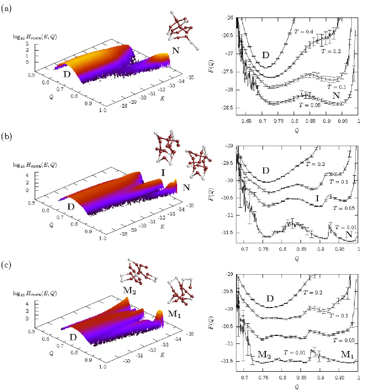
Figure 5: Multicanonical histograms $H_{\text{muca}}(E,Q)$ of energy $E$ and angular overlap parameter $Q$ and free-energy landscapes $F(Q)$ at different temperatures for the three sequences (see Table 1) (a) S1, (b) S2, and (c) S3. The reference folds reside at $Q=1$ and $E=E_{\text{min}}$. Pseudophases are symbolized by D (denatured states), N (native folds), I (intermediates), and M (metastable states). Representative conformations in intermediate and folded phases are also shown ssbj1 .

Interpreting the ridges of the probability distributions in the left-hand panel of Fig. 5 as folding channels, it can clearly be seen that the heteropolymers exhibit noticeable differences in the folding behavior towards the native conformations (N). Considering natural proteins it would not be surprising that different sequences of amino acids cause in many cases not only different native folds but also vary in their folding behavior. Here we are considering, however, a highly minimalistic heteropolymer model and hitherto it is not obvious that it is indeed possible to separate characteristic folding channels in this simple model, but as Fig. 5 demonstrates, in fact, it is. For sequence S1, we identify in Fig. 5(a) a typical two-state characteristics. Approaching from high energies (or high temperatures), the conformations in the ensemble of denatured conformations (D) have an angular overlap $Q\approx 0.7$, which means that there is no significant similarity with the reference structure, i.e., the ensemble D consists mainly of unfolded peptides. For energies $E<-30$ a second branch opens. This channel (N) leads to the native conformation (for which $Q=1$ and $E_{\text{min}}\approx-33.8$). The constant-energy distribution, where the main and native-fold channels D and N coexist, exhibits two peaks noticeably separated by a well. Therefore, the conformational transition between the channels looks first-order-like, which is typical for two-state folding. The main channel D contains the ensemble of unfolded conformations, whereas the native-fold channel N represents the folded states.

The two-state behavior is confirmed by analyzing the temperature dependence of the minima in the free-energy landscape. The free energy as a function of the “order” parameter $Q$ at fixed temperature can be suitably defined as:

$$F(Q)=-k_{B}T\ln p(Q).$$ (11)

In this expression,

$$p(Q^{\prime})=\int{\cal D}{\bf X}\,\delta(Q^{\prime}-Q({\bf X},{\bf X}^{(0)}))\,e^{-E({\bf X})/k_{B}T}$$ (12)

is related to the probability of finding a conformation with a given value of $Q$ in the canonical ensemble at temperature $T$. The formal integration runs over all possible conformations ${\bf X}$. In the right-hand panel of Fig. 5(a), the free-energy landscape at various temperatures is shown for sequence S1. At comparatively high temperatures ($T=0.4$), only the unfolded states ($Q\approx 0.71$) in the main folding channel D dominate. Decreasing the temperature, the second (native-fold) channel N begins to form ($Q\approx 0.9$), but the global free-energy minimum is still associated with the main channel. Near $T\approx 0.1$, both free-energy minima have approximately the same value, the folding transition occurs. The discontinuous character of this conformational transition is manifest by the existence of the free-energy barrier between the two macrostates. For even smaller temperatures, the native-fold-like conformations ($Q>0.95$) dominate and fold smoothly towards the $Q=1$ reference conformation, which is the lowest-energy conformation found in the simulation.

A significantly different folding behavior is noticed for the heteropolymer with sequence S2. The corresponding multicanonical histogram is shown in Fig. 5(b) and represents a folding event through an intermediate macrostate. The main channel D bifurcates and a side channel I branches off continuously. This branching is followed by the formation of a third channel N, which ends in the native fold. The characteristics of folding-through-intermediates is also confirmed by the free-energy landscapes as shown for this sequence in Fig. 5(b) at different temperatures. Approaching from high temperatures, the ensemble of denatured conformations D ($Q\approx 0.76$) is dominant. Close to the transition temperature $T\approx 0.05$, the intermediary phase I is reached. The overlap of these intermediary conformations with the native fold is about $Q\approx 0.9$. Decreasing the temperature further below the native-folding threshold close to $T=0.01$, the hydrophobic-core formation is finished and stable native-fold-like conformations with $Q>0.97$ dominate (N).

The most extreme behavior of the three exemplified sequences is exhibited by the heteropolymer S3. Figure 5(c) shows that the main channel D does not decay in favor of a native-fold channel. In fact, we observe both, the formation of two separate native-fold channels M${}_{\text{1}}$ and M${}_{\text{2}}$. Channel M${}_{\text{1}}$ advances towards the $Q=1$ fold and M${}_{\text{2}}$ ends up in a completely different conformation with approximately the same energy ($E\approx-33.5$). The spatial structures of these two conformations are noticeably different and their mutual overlap is correspondingly very small, $Q\approx 0.75$. It should also be noted that the lowest-energy conformations in the main channel D have only slightly larger energies than the two native folds. Thus, the folding of this heteropolymer is accompanied by a very complex folding characteristics. In fact, this multiple-peak distribution near minimum energies is a strong indication for metastability. A native fold in the natural sense does not exist, the $Q=1$ conformation is only a reference state but the folding towards this structure is not distinguished as it is in the folding characteristics of sequences S1 and S2. The amorphous folding behavior is also seen in the free-energy landscapes in Fig. 5(c). Above the folding transitions ($T=0.2$) the typical sequence-independent denatured conformations with $\langle Q\rangle\approx 0.77$ dominate (D). Then, in the annealing process, several channels are formed and coexist. The two most prominent channels (to which the lowest-energy conformations belong that we found in the simulations) eventually lead for $T\approx 0.01$ to ensembles of macrostates with $Q>0.97$ (M${}_{\text{1}}$), and conformations with $Q<0.75$ (M${}_{\text{2}}$). The lowest-energy conformation found in this regime is structurally different but energetically degenerate, if compared with the reference conformation.

7 Statistical analyses of peptide aggregation

7.1 Pseudophase separation in polymeric nucleation processes

Beside folding mechanisms, the aggregation of proteins belongs to the biologically most relevant molecular structure formation processes. While the specific docking between receptors and ligands is not necessarily accompanied by global structural changes, protein folding and oligomerization of peptides are typically cooperative conformational transitions gsponer1 . Proteins and their aggregates are comparatively small systems and are often formed by only a few peptides. A very prominent example is the extracellular aggregation of the A$\beta$ peptide, which is associated with Alzheimer’s disease. Following the amyloid hypothesis, it is believed that these aggregates are neurotoxic, i.e., they are able to fuse into cell membranes of neurons and open calcium ion channels. It is known that extracellular Ca²⁺ ions intruding into a neuron can promote its degeneration lin1 ; quist1 ; lashuel1 .

Conformational transitions proteins experience during structuring and aggregation are not phase transitions in the strict thermodynamic sense and their statistical analysis is usually based on studies of signals exposed by energetic and structural fluctuations, as well as system-specific “order” parameters. In these studies, the temperature $T$ is considered as an adjustable, external control parameter and, for the analysis of the pseudophase transitions, the peak structure of quantities such as the specific heat and the fluctuations of the gyration tensor components or “order” parameter as functions of the temperature are investigated. The natural ensemble for this kind of analysis is the canonical ensemble, where the possible states of the system with energies $E$ are distributed according to the Boltzmann probability $\exp(-E/k_{B}T)$, where $k_{B}$ is the Boltzmann constant. However, phase separation processes of small systems are accompanied by surface effects at the interface between the pseudophases gross1 ; gross2 . This is reflected by the behavior of the microcanonical entropy ${\cal S}(E)$, which exhibits a convex monotony in the transition region. Consequences are the backbending of the caloric temperature $T(E)=(\partial{\cal S}/\partial E)^{-1}$, i.e., the decrease of temperature with increasing system energy, and the negativity of the microcanonical specific heat $C_{V}(E)=(\partial T(E)/\partial E)^{-1}=-(\partial{\cal S}/\partial E)^{2}/(\partial^{2}{\cal S}/\partial E^{2})$. The physical reason is that the free energy balance in phase equilibrium requires the minimization of the interfacial surface and, therefore, the loss of entropy gross3 ; jbj1 ; jbj2 . A reduction of the entropy can, however, only be achieved by transferring energy into the system.

It is a surprising fact that this so-called backbending effect is indeed observed in transitions with phase separation. Although this phenomenon has already been known for a long time from astrophysical systems thirring1 , it has been widely ignored since then as somehow “exotic” effect. Recently, however, experimental evidence was found from melting studies of sodium clusters by photofragmentation schmidt1 . Bimodality and negative specific heats are also known from nuclei fragmentation experiments and models pichon1 ; lopez1 , as well as from spin models on finite lattices which experience first-order transitions in the thermodynamic limit wj1 ; pleimling1 . This phenomenon is also observed in a large number of other isolated finite model systems for evaporation and melting effects wales1 ; hilbert1 .

The following discussion of the aggregation behavior is based on multicanonical computer simulations of a mesoscopic hydrophobic-polar heteropolymer model for aggregation based on the AB model jbj1 ; jbj2 .

7.2 Mesoscopic hydrophobic-polar aggregation model

For studies of heteropolymer aggregation on mesoscopic scales, a novel model is employed that is based on the hydrophobic-polar single-chain AB model (4). As for modeling heteropolymer folding, we assume here that the tertiary folding process of the individual chains is governed by hydrophobic-core formation in an aqueous environment. For systems of more than one chain, we further take into account that the interaction strengths between nonbonded residues are independent of the individual properties of the chains the residues belong to. Therefore, we use the same parameter sets as in the AB model for the pairwise interactions between residues of different chains. Our aggregation model reads jbj1 ; jbj2

$$E=\sum\limits_{\mu}E_{\text{AB}}^{(\mu)}+\sum\limits_{\mu<\nu}\sum_{i_{\mu},j_{\nu}}\Phi(r_{i_{\mu}j_{\nu}};\sigma_{i_{\mu}},\sigma_{j_{\nu}}),$$ (13)

where $\mu,\nu$ label the $M$ polymers interacting with each other, and $i_{\mu},j_{\nu}$ index the $N_{\mu,\nu}$ monomers of the respective $\mu$th and $\nu$th polymer. The intrinsic single-chain energy of the $\mu$th polymer is given by [cf. Eq. (4)]

$$E_{\text{AB}}^{(\mu)}=\frac{1}{4}\sum\limits_{i_{\mu}}(1-\cos\vartheta_{i_{\mu}})+\!\!\sum\limits_{j_{\mu}>i_{\mu}+1}\Phi(r_{i_{\mu}j_{\mu}};\sigma_{i_{\mu}},\sigma_{j_{\mu}}),$$ (14)

with $0\leq\vartheta_{i_{\mu}}\leq\pi$ denoting the bending angle between monomers $i_{\mu}$, $i_{\mu}+1$, and $i_{\mu}+2$. The nonbonded inter-residue pair potential

$$\Phi(r_{i_{\mu}j_{\nu}};\sigma_{i_{\mu}},\sigma_{j_{\nu}})=4\left[r_{i_{\mu}j_{\nu}}^{-12}-C(\sigma_{i_{\mu}},\sigma_{j_{\nu}})r_{i_{\mu}j_{\nu}}^{-6}\right]$$ (15)

depends on the distance $r_{i_{\mu}j_{\nu}}$ between the residues, and on their type, $\sigma_{i_{\mu}}=A,B$. The long-range behavior is attractive for like pairs of residues [$C(A,A)=1$, $C(B,B)=0.5$] and repulsive otherwise [$C(A,B)=C(B,A)=-0.5$]. The lengths of all virtual peptide bonds are set to unity.

Employing this model, we study in the following thermodynamic properties of the aggregation of oligomers with the Fibonacci sequence F1: $AB_{2}AB_{2}ABAB_{2}AB$ over the whole energy and temperature regime.

7.3 Order parameter of aggregation and fluctuations

In order to distinguish between the fragmented and the aggregated regime, we introduce the “order” parameter jbj1 ; jbj2

$$\Gamma^{2}=\frac{1}{2M^{2}}\sum_{\mu,\nu=1}^{M}{\bf d}_{\text{per}}^{2}\left({\bf r}_{\text{COM},\mu},{\bf r}_{\text{COM},\nu}\right),$$ (16)

where the summations are taken over the minimum distances ${\bf d}_{\text{per}}=\left(d_{\text{per}}^{(1)},d_{\text{per}}^{(2)},d_{\text{per}}^{(3)}\right)$ of the respective centers of mass of the chains (or their periodic continuations). The center of mass of the $\mu$th chain in a box with periodic boundary conditions is defined as ${\bf r}_{\text{COM},\mu}=\sum_{i_{\mu}=1}^{N_{\mu}}\left[{\bf d}_{\text{per}}\left({\bf r}_{i_{\mu}},{\bf r}_{1_{\mu}}\right)+{\bf r}_{1_{\mu}}\right]/N_{\mu}$, where ${\bf r}_{1_{\mu}}$ is the coordinate vector of the first monomer and serves as a reference coordinate in a local coordinate system.

The aggregation parameter is to be considered as a qualitative measure; roughly, fragmentation corresponds to large values of $\Gamma$, aggregation requires the centers of masses to be close to each other, in which case $\Gamma$ is comparatively small. Despite its qualitative nature, it turns out to be a surprisingly manifest indicator for the aggregation transition and allows even a clear discrimination of different aggregation pathways, as will be seen later on.

According to the Boltzmann distribution, we define canonical expectation values of any observable $O$ by

$$\langle O\rangle(T)=\frac{1}{Z_{\text{can}}(T)}\prod\limits_{\mu=1}^{M}\left[\int{\cal D}{\bf X}_{\mu}\right]O(\{{\bf X}_{\mu}\})e^{-E(\{{\bf X}_{\mu}\})/k_{B}T},$$ (17)

where the canonical partition function $Z_{\text{can}}$ is given by

$$Z_{\text{can}}(T)=\prod\limits_{\mu=1}^{M}\left[\int{\cal D}{\bf X}_{\mu}\right]e^{-E(\{{\bf X}_{\mu}\})/k_{B}T}.$$ (18)

Formally, the integrations are performed over all possible conformations ${\bf X}_{\mu}$ of the $M$ chains.

Similarly to the specific heat per monomer $c_{V}(T)=d\langle E\rangle/N_{\text{tot}}dT=(\langle E^{2}\rangle-\langle E\rangle^{2})/N_{\text{tot}}k_{B}T^{2}$ (with $N_{\text{tot}}=\sum_{\mu=1}^{M}N_{\mu}$) which expresses the thermal fluctuations of energy, the temperature derivative of $\langle\Gamma\rangle$ per monomer, $d\langle\Gamma\rangle/N_{\text{tot}}dT=(\langle\Gamma E\rangle-\langle\Gamma\rangle\langle E\rangle)/N_{\text{tot}}k_{B}T^{2}$, is a useful indicator for cooperative behavior of the multiple-chain system. Since the system size is small – the number of monomers $N_{\text{tot}}$ as well as the number of chains $M$ – aggregation transitions, if any, are expected to be signalized by the peak structure of the fluctuating quantities as functions of the temperature. This requires the temperature to be a unique external control parameter which is a natural choice in the canonical statistical ensemble. Furthermore, this is a typically easily adjustable and, therefore, convenient parameter in experiments. However, aggregation is a phase separation process and, since the system is small, there is no uniform mapping between temperature and energy jbj1 ; jbj2 . For this reason, the total system energy is the more appropriate external parameter. Thus, the microcanonical interpretation will turn out to be the more favorable description, at least in the transition region.

7.4 Canonical and microcanonical interpretation

Figure 6: Aggregation parameter $\langle\Gamma\rangle/N_{\text{tot}}$ and fluctuations $d\langle\Gamma\rangle/N_{\text{tot}}dT$ as functions of the temperature.

In our aggregation study of the 2$\times$F1 system we obtain from the canonical analysis a surprisingly clear picture of the aggregation transition. In Fig. 6, the temperature dependence of the mean aggregation order parameter $\langle\Gamma\rangle$ and the fluctuations of $\Gamma$ are shown. The aggregation transition is signalized by a very sharp peak and we read off an aggregation temperature close to $T_{\text{agg}}\approx 0.20$. The aggregation of the two peptides is a single-step process, in which the formation of the aggregate with a common compact hydrophobic core governs the folding behavior of the individual chains. Under such conditions, folding and binding are not separate processes. This is different if the intrinsic polymeric forces are stronger than the binding affinity. In this case the already folded molecule simply docks at the active site of a target without changing its global conformation. These two principal scenarios are also observed in molecular adsorption processes at solid substrates. This provides another example where mesoscopic models prove extremely useful in order to reveal the structural phases of adsorbed and desorbed conformations in dependence of external parameters such as solvent quality and temperature adbj1 ; adbj2 .

In the microcanonical analysis of peptide-peptide aggregation, the system energy $E$ is kept (almost) fixed and treated as an external control parameter. The system can only take macrostates with energies in the interval $(E,E+\Delta E)$ with $\Delta E$ being sufficiently small to satisfy $\Delta G(E)=g(E)\Delta E$, where $\Delta G(E)$ is the phase-space volume of this energetic shell. In the limit $\Delta E\to 0$, the total phase-space volume up to the energy $E$ can thus be expressed as

$$G(E)=\int_{E_{\text{min}}}^{E}dE^{\prime}\,g(E^{\prime}).$$ (19)

Since $g(E)$ is positive for all $E$, $G(E)$ is a monotonically increasing function and this quantity is suitably related to the microcanonical entropy ${\cal S}(E)$ of the system. In the definition of Hertz,

$${\cal S}(E)=k_{B}\ln\,G(E).$$ (20)

Alternatively, the entropy is often directly related to the density of states $g(E)$ and defined as

$$S(E)=k_{B}\ln\,g(E).$$ (21)

The density of states exhibits a decrease much faster than exponential towards the low-energy states. For this reason, the phase-space volume at energy $E$ is strongly dominated by the number of states in the energy shell $\Delta E$. Thus $G(E)\approx\Delta G(E)\sim g(E)$ is directly related to the density of states. This virtual identity breaks down in the higher-energy region, where $\ln\,g(E)$ is getting flat – in our case far above the energetic regions being relevant for the discussion of the aggregation transition (i.e., for energies $E\gg E_{\text{frag}}$, see Fig. 7). Actually, both definitions of the entropy lead to virtually identical results in the analysis of the aggregation transition jbj1 ; jbj2 . The (reciprocal) slope of the microcanonical entropy fixes the temperature scale and the corresponding caloric temperature is then defined via $T(E)=(\partial{\cal S}(E)/\partial E)^{-1}$ for fixed volume $V$ and particle number $N_{\text{tot}}$.

Figure 7: Microcanonical Hertz entropy ${\cal S}(E)$ of the 2$\times$F1 system, concave Gibbs hull ${\cal H}_{\cal S}(E)$, and inverse caloric temperature $T^{-1}(E)$ as functions of energy. The phase separation regime ranges from $E_{\text{agg}}$ to $E_{\text{frag}}$. Between $T^{-1}_{<}$ and $T^{-1}_{>}$, the temperature is no suitable external control parameter and the canonical interpretation is not useful: The inverse caloric temperature $T^{-1}(E)$ exhibits an obvious backbending in the transition region. Note the second, less-pronounced backbending in the energy range $E_{<}<E<E_{\text{frag}}$.

As long as the mapping between the caloric temperature $T$ and the system energy $E$ is bijective, the canonical analysis of crossover and phase transitions is suitable since the temperature can be treated as external control parameter. For systems, where this condition is not satisfied, however, in a standard canonical analysis one may easily miss a physical effect accompanying condensation processes: Due to surface effects (the formation of the contact surface between the peptides requires a rearrangement of monomers in the surfaces of the individual peptides), additional energy does not necessarily lead to an increase of temperature of the condensate. Actually, the aggregate can even become colder. The supply of additional energy supports the fragmentation of parts of the aggregate, but this is overcompensated by cooperative processes of the particles aiming to reduce the surface tension. Condensation processes are phase-separation processes and as such aggregated and fragmented phases coexist. Since in this phase-separation region $T$ and $E$ are not bijective, this phenomenon is called the “backbending effect”. The probably most important class of systems exhibiting this effect is characterized by their smallness and the capability to form aggregates, depending on the interaction range. The fact that this effect could be indirectly observed in sodium clustering experiments schmidt1 gives rise to the hope that backbending could also be observed in aggregation processes of small peptides.

Since the 2$\times$F1 system apparently belongs to this class, the backbending effect is also observed in the aggregation/fragmentation transition of this system. This is shown in Fig. 7, where the microcanonical entropy ${\cal S}(E)$ is plotted as function of the system energy. The phase-separation region of aggregated and fragmented conformations lies between $E_{\text{agg}}\approx-8.85$ and $E_{\text{frag}}\approx 1.05$. Constructing the concave Gibbs hull ${\cal H}_{\cal S}(E)$ by linearly connecting ${\cal S}(E_{\text{agg}})$ and ${\cal S}(E_{\text{frag}})$ (straight dashed line in Fig. 7), the entropic deviation due to surface effects is simply $\Delta{\cal S}(E)={\cal H}_{\cal S}(E)-{\cal S}(E)$. The deviation is maximal for $E=E_{\text{sep}}$ and $\Delta{\cal S}(E_{\text{sep}})\equiv\Delta{\cal S}_{\text{surf}}$ is the surface entropy. The Gibbs hull also defines the aggregation transition temperature

$$T_{\text{agg}}=\left(\frac{\partial{\cal H}_{\cal S}(E)}{\partial E}\right)^{-1}.$$ (22)

For the 2$\times$F1 system, we find $T_{\text{agg}}\approx 0.198$, which is virtually identical with the peak temperature of the aggregation parameter fluctuation (see Fig. 6).

The inverse caloric temperature $T^{-1}(E)$ is also plotted into Fig. 7. For a fixed temperature in the interval $T_{<}<T<T_{>}$ ($T_{<}\approx 0.169$ and $T_{>}\approx 0.231$), different energetic macrostates coexist. This is a consequence of the backbending effect. Within the backbending region, the temperature decreases with increasing system energy. The horizontal line at $T^{-1}_{\text{agg}}\approx 5.04$ is the Maxwell construction, i.e., the slope of the Gibbs hull ${\cal H}_{\cal S}(E)$. Although the transition seems to have similarities with the van der Waals description of the condensation/evaporation transition of gases – the “overheating” of the aggregate between $T_{\text{agg}}$ and $T_{>}$ (within the energy interval $E_{\text{agg}}<E<E_{>}\approx-5.13$) is as apparent as the “undercooling” of the fragments between $T_{<}$ and $T_{\text{agg}}$ (in the energy interval $E_{\text{frag}}>E>E_{<}\approx-1.13$) – it is important to notice that in contrast to the van der Waals picture the backbending effect in-between is a real physical effect. Another essential result is that in the transition region the temperature is not a suitable external control parameter: The macrostate of the system cannot be adjusted by fixing the temperature. The better choice is the system energy which is unfortunately difficult to control in experiments. Another direct consequence of the energetic ambiguity for a fixed temperature between $T_{<}$ and $T_{>}$ is that the canonical interpretation is not suitable for detecting the backbending phenomenon.

The most remarkable result is the negativity of the specific heat of the system in the backbending region, as shown in Fig. 8. A negative specific heat in the phase separation regime is due to the nonadditivity of the energy of the two subsystems as the interaction between the chains is stronger than the attractive inter-chain forces of the individual polymers. “Heating” a large aggregate would lead to the stretching of monomer-monomer contact distances, i.e., the potential energy of an exemplified pair of monomers increases, while kinetic energy and, therefore, temperature remain widely constant. In a comparatively small aggregate, additional energy leads to cooperative rearrangements of monomers in the aggregate in order to reduce surface tension, i.e, the formation of molten globular aggregates is suppressed. In consequence, kinetic energy is transferred into potential energy and the temperature decreases. In this regime, the aggregate becomes colder, although the total energy increases  jbj1 .

Figure 8: Microcanonical specific heat $C_{V}(E)$ for the 2$\times$F1 complex. Note the negativity in the backbending regions jbj1 .

The precise microcanonical analysis reveals also a further detail of the aggregation transition. Close to $E_{\text{pre}}\approx-0.32$, the $T^{-1}$ curve in Fig. 7 exhibits another “backbending” which signalizes a second, but unstable transition of the same type. The associated transition temperature $T_{\text{pre}}\approx 0.18$ is smaller than $T_{\text{agg}}$, but this transition occurs in the energetic region where fragmented states dominate. Thus this transition can be interpreted as the premelting of aggregates by forming intermediate states. These intermediate structures are rather weakly stable: The population of the premolten aggregates never dominates. In particular, at $T_{\text{pre}}$, where premolten aggregates and fragments coexist, the population of compact aggregates is much larger. This can nicely be seen in the canonical energy histograms at these temperatures plotted in Fig. 9, where the second backbending is only signalized by a small cusp in the coexistence region. Since both transitions are phase-separation processes, structure formation is accompanied by releasing latent heat which can be defined as the energetic widths of the phase coexistence regimes, i.e., $\Delta Q_{\text{agg}}=E_{\text{frag}}-E_{\text{agg}}=T_{\text{agg}}[{\cal S}(E_{\text{frag}})-{\cal S}(E_{\text{agg}})]\approx 9.90$ and $\Delta Q_{\text{pre}}=E_{\text{frag}}-E_{\text{pre}}=T_{\text{pre}}[{\cal S}(E_{\text{frag}})-{\cal S}(E_{\text{pre}})]\approx 1.37$. Obviously, the energy required to melt the premolten aggregate is much smaller than to dissolve a compact (solid) aggregate.

Figure 9: Logarithmic plots of the canonical energy histograms (not normalized) at $T\approx 0.18$ and $T\approx 0.20$, respectively.

For the comparison of the surface entropies, we use the definition (21) of the entropy. In the case of the aggregation transition, the surface entropy is $\Delta{\cal S}_{\text{surf}}^{\text{agg}}\approx\Delta S_{\text{surf}}^{\text{agg}}=H_{S}(E_{\text{sep}})-S(E_{\text{sep}})$, where $H_{S}(E)\approx{\cal H}_{\cal S}(E)$ is the concave Gibbs hull of $S(E)$. Since $H_{S}(E_{\text{sep}})=H_{S}(E_{\text{frag}})-(E_{\text{frag}}-E_{\text{sep}})/T_{\text{agg}}$ and $H_{S}(E_{\text{frag}})=S(E_{\text{frag}})$, the surface entropy is

$$\Delta S_{\text{surf}}^{\text{agg}}=S(E_{\text{frag}})-S(E_{\text{sep}})-\frac{1}{T_{\text{agg}}}(E_{\text{frag}}-E_{\text{sep}}).$$ (23)

Yet utilizing that the canonical distribution $h_{\text{can}}(E)=\int d\Gamma\,H_{\text{can}}(E,\Gamma;T)$ at $T_{\text{agg}}$ (shown in Fig. 9) is $h_{\text{can}}(E)\sim g(E)\exp(-E/k_{B}T_{\text{agg}})$, the surface entropy can be written in the simple and computationally convenient form wj1 :

$$\Delta S_{\text{surf}}^{\text{agg}}=k_{B}\ln\,\frac{h_{\text{can}}(E_{\text{frag}})}{h_{\text{can}}(E_{\text{sep}})}.$$ (24)

A similar expression is valid for the coexistence of premolten and fragmented states at $T_{\text{pre}}$ The corresponding canonical distribution is also shown in Fig. 9. Thus, we obtain (in units of $k_{B}$) for the surface entropy of the aggregation transition $\Delta S_{\text{surf}}^{\text{agg}}\approx 2.48$ and for the premelting $\Delta S_{\text{surf}}^{\text{pre}}\approx 0.04$, confirming the weakness of the interface between premolten aggregates and fragmented states.

7.5 Aggregation transition in larger heteropolymer systems

The statements in the previous section for the 2$\times$F1 system are also, in general, valid for larger systems. This is the result of computer simulations for systems consisting of three (in the following referred to as 3$\times$F1) and four (4$\times$F1) identical peptides with sequence F1. As it has already been discussed for the 2$\times$F1 system, there are also for the larger systems no obvious signals for separate aggregation and hydrophobic-core formation processes. Only weak activity in the energy fluctuations in the temperature region below the aggregation transition temperature indicates that local restructuring processes of little cooperativity (comparable with the discussion of the premolten aggregates in the discussion of the 2$\times$F1 system) are still happening. The strength of the aggregation transition is also documented by the fact that the peak temperatures of energetic and aggregation parameter fluctuations are virtually identical for the multi-peptide systems, i.e., the aggregation temperature is $T_{\text{agg}}\approx 0.2$.

In Fig. 10, the microcanonical entropies per monomer $s(e)={\cal S}(e)/N_{\text{tot}}$ (shifted by an unimportant constant for clearer visibility) and the corresponding Gibbs hulls $h_{s}(e)={\cal H}_{\cal S}(e)/N_{\text{tot}}$ are shown for 2$\times$F1 (in the figure denoted by “2”), 3$\times$F1 (“3”), and 4$\times$F1 (“4”), respectively, as functions of the energy per monomer $e=E/N_{\text{tot}}$. Although the convex entropic “intruder” is apparent for larger systems as well, its relative strength decreases with increasing number of chains. The slopes of the respective Gibbs constructions determine the aggregation temperature (22) which are found to be $T_{\text{agg}}^{\text{3}\times\text{F1}}\approx 0.212$ and $T_{\text{agg}}^{\text{4}\times\text{F1}}\approx 0.217$.

Figure 10: Microcanonical entropies per monomer $s(e)$, respective Gibbs constructions $h_{s}(e)$ (left-hand scale), and deviations $\Delta s(e)=h_{s}(e)-s(e)$ (right-hand scale) for 2$\times$F1 (labeled as 2), 3$\times$F1 (3), and 4$\times$F1 (4) as functions of the energy per monomer $e$.

The existence of the interfacial boundary entails a transition barrier whose strength is characterized by the surface entropy $\Delta{\cal S}_{\text{surf}}$. In Fig. 10, the individual entropic deviations per monomer, $\Delta s(e)=\Delta{\cal S}(e)/N_{\text{tot}}$ are also shown and the maximum deviations, i.e., the surface entropies $\Delta{\cal S}_{\text{surf}}$ and relative surface entropies per monomer $\Delta s_{\text{surf}}=\Delta{\cal S}_{\text{surf}}/N_{\text{tot}}$ are listed in Table 2. There is no apparent difference between the values of $\Delta{\cal S}_{\text{surf}}$ that would indicate a trend for a vanishing of the absolute surface barrier in larger systems. However, the relative surface entropy $\Delta s_{\text{surf}}$ obviously decreases. Whether or not it vanishes in the thermodynamic limit cannot be decided from our present results and is a study worth in its own right.

It is also interesting that subleading effects increase and the double-well form found for 2$\times$F1 changes by higher-order effects, and it seems that for larger systems the almost single-step aggregation of 2$\times$F1 is replaced by a multiple-step process.

Table 2: Aggregation temperatures $T_{\text{agg}}$, surface entropies $\Delta{\cal S}_{\text{surf}}$, relative surface entropies per monomer $\Delta s_{\text{surf}}$, relative aggregation and fragmentation energies per monomer, $e_{\text{agg}}$ and $e_{\text{frag}}$, respectively, latent heat per monomer $\Delta q$, and phase-separation entropy per monomer $\Delta q/T_{\text{agg}}$. All quantities for systems consisting of two, three, and four 13-mers with AB sequence F1.

system	$T_{\text{agg}}$	$\Delta{\cal S}_{\text{surf}}$	$\Delta s_{\text{surf}}$	$e_{\text{agg}}$	$e_{\text{frag}}$	$\Delta q$	$\Delta q/T_{\text{agg}}$
2$\times$F1	0.198	2.48	0.10	$-$0.34	0.04	0.38	1.92
3$\times$F1	0.212	2.60	0.07	$-$0.40	0.05	0.45	2.12
4$\times$F1	0.217	2.30	0.04	$-$0.43	0.05	0.48	2.21

Not surprisingly, the fragmented phase is hardly influenced by side effects and the rightmost minimum in Fig. 10 lies well at $e_{\text{frag}}=E_{\text{frag}}/N_{\text{tot}}\approx 0.04-0.05$. Since the Gibbs construction covers the whole convex region of $s(e)$, the aggregation energy per monomer $e_{\text{agg}}=E_{\text{agg}}/N_{\text{tot}}$ corresponds to the leftmost minimum and its value changes noticeably with the number of chains. In consequence, the latent heat per monomer $\Delta q=\Delta Q/N_{\text{tot}}=T_{\text{agg}}[{\cal S}(E_{\text{frag}})-{\cal S}(E_{\text{agg}})]/N_{\text{tot}}$ that is required to fragment the aggregate increases from two to four chains in the system (see Table 2). Although the systems under consideration are too small to extrapolate phase transition properties in the thermodynamic limit, it is obvious that the aggregation-fragmentation transition exhibits strong similarities to condensation-evaporation transitions of colloidal systems. Given that, the entropic transition barrier $\Delta q/T_{\text{agg}}$, which we see increasing with the number of chains (cf. the values in Table 2), would survive in the thermodynamic limit and the transition was first-order-like. More surprising would be, however, if the convex intruder would not disappear, i.e., if the absolute and relative surface entropies $\Delta{\cal S}_{\text{surf}}$ and $\Delta s_{\text{surf}}$ do not vanish. This is definitely a question of fundamental interest as the common claim is that pure surface effects typically exhibited only by “small” systems are irrelevant in the thermodynamic limit. This requires studies of much larger systems.

It should clearly be noted, however, that protein aggregates forming themselves in biological systems often consist only of a few peptides and are definitely of small size and the surface effects are responsible for structure formation and are not unimportant side effects. One should keep in mind that standard thermodynamics and the thermodynamic limit are somewhat theoretical constructs valid only for very large systems. The increasing interest in physical properties of small systems, in particular in conformational transitions in molecular systems, requires in part a revision of dogmatic thermodynamic views. Indeed, by means of today’s chemo-analytical and experimental equipment, effects like those described in this chapter, should actually experimentally be verifiable as these are real physical effects. For studies of the condensation of atoms, where a similar behavior occurs, such experiments have actually already been performed schmidt1 .

8 Summary

The analyses in the previous sections have shown that it is indeed possible to reveal characteristic features of structure formation processes of polymers, in particular proteins, by means of minimalistic coarse-grained models. This is essential, as a generalized view of conformational transitions occurring in folding and aggregation processes of molecular systems can only possess a solid basis, if a classification of generic features common to different systems enables the introduction of suitable models on mesoscopic scales.

Depending on the heteropolymer sequence, typically two general transitions occur in heteropolymer folding processes. One is the folding transition from random coils to compact globular conformations common to all heteropolymers (i.e., little sequence-specific), a finite-length analog to the collapse (or $\Theta$) transition known from homopolymers. The stability of the globular or intermediary (pseudo)phase of heteropolymers depends, however, strongly on the heteropolymer sequence. The second general transition at lower temperature (or worse solvent quality) is sort of a glassy transition as it results in the formation of the native conformation(s) with small entropy. During this transition, the highly compact hydrophobic core is formed, surrounded by a shell of polar residues which screens the core from the solvent. The kinetics of this transition strongly depends on the heteropolymer sequence. Hydrophobic-core formation is typically a (“first-order-like”) phase separation process and the sharpness and height of the free-energy barrier separating the hydrophobic-core and globular (pseudo)phases are measures for the stability of the hydrophobic core. It is assumed that a large set of the comparatively few functional bioproteins in nature exhibits such a large barrier preventing unfolding into nonfunctional conformations. This is also one of the common arguments, why under physiological conditions only a very small number among the possible protein sequences can be functional at all.

Although the mesoscopic models are still extremely minimalistic, we have found quite surprising characteristic folding features comparable to those of real proteins. Analyzing transition channels and free-energy landscapes based on a suitably defined similarity or “order” parameter, we identified folding behaviors which are known from real proteins in a like manner: two-state folding with a single kinetic barrier and unique native state, folding towards the native fold through intermediates over different barriers, and metastability with different, almost degenerate, native states.

We have also discussed in detail thermodynamic properties of peptide aggregation processes. We compared small systems of different numbers of short peptides and investigated finite-size properties in the canonical and in the microcanonical ensemble. Each of these analyses has advantages. Applying the canonical formalism reveals strong fluctuations in the vicinity of the aggregation transition which allow for a precise estimation of the aggregation transition temperature for a finite system, but also for a finite-size scaling analysis toward the system with infinitely many chains.

But, analyzing the aggregation of a few peptides from the microcanonical perspective uncovers an underlying physical effect, the backbending effect, which is largely “averaged out” in the canonical analysis. “Backbending” means that in the transition region the caloric temperature decreases with increasing energy. This is due to surface effects, additional energy does not lead to an increase of the caloric temperature; rather it is used to rearrange monomers in order to reduce surface tension at the expense of entropy. In effect, the protein complex is getting colder. For an increasing number of peptides in the system, we could show, however, that the effect becomes less relevant, although the latent heat increases and thus the first-order character of this phase-separation process is getting stronger. Nonetheless, in biological aggregation processes typically only a few proteins are involved and thus the effect should be apparent. The “physical reality” of this effect has already been confirmed in atomic cluster formation experiments. However, the experimental verification in polymeric systems is still pending.

One of the essential questions in aggregation processes among polymers is, how the mutual influence induces conformational changes. Two potential scenarios leading to the formation of complexes are conceivable. If the external force is attractive, but weaker than the intrinsic, intermonomeric forces that form the polymer or protein conformation, the proximity of an attractive polymer or substrate is not sufficient to refold the polymer and the aggregation is a simple docking process. Unless the match is perfect, the binding force that holds the compound together is rather weak. On the other hand, if the external force entails refolding of the polymer, it can better adapt to the target structure (e.g., a crystalline substrate), or, if both partners experience conformational changes, a new, highly compact compound can form. In this so-called coupled folding-binding process, the binding force is typically stronger than in the docking case. In our aggregation study of a few short peptides, we observed such a behavior.

Our results were mainly obtained by means of sophisticated generalized-ensemble chain-growth and Markov chain Monte Carlo computer simulations, partly newly developed or generalized for these purposes. It is a non-negligible fact that even with today’s equipment computer simulations of polymers, in particular, proteins, are extremely demanding and efficient algorithms are required. Despite the enormous progress in protein research in the past few years, it will remain one of the biggest scientific future challenges to uncover the principal secrets of cooperative conformational activity in structure formation processes of proteins.

References

- (1) E. Shakhnovich, Chem. Rev. 106, 1559 (2006).
- (2) M. Bachmann and W. Janke, Lect. Notes Phys. 736, 203 (2008).
- (3) C. Tang, Physica A 288, 31 (2000).
- (4) K. A. Dill, Biochemistry 24, 1501 (1985); K. F. Lau and K. A. Dill, Macromolecules 22, 3986 (1989).
- (5) R. Schiemann, M. Bachmann, and W. Janke, J. Chem. Phys. 122, 114705 (2005); Comp. Phys. Commun. 166, 8 (2005).
- (6) M. Bachmann and W. Janke, Phys. Rev. Lett. 91, 208105 (2003); J. Chem. Phys. 120, 6779 (2004).
- (7) K. Yue and K. A. Dill, Phys. Rev. E 48, 2267 (1993); Proc. Natl. Acad. Sci. (USA) 92, 146 (1995).
- (8) R. Unger and J. Moult, J. Mol. Biol. 231, 75 (1993).
- (9) K. Yue, K. M. Fiebig, P. D. Thomas, H. S. Chan, E. I. Shakhnovich, and K. A. Dill, Proc. Natl. Acad. Sci. (USA) 92, 325 (1995).
- (10) E. E. Lattman, K. M. Fiebig, and K. A. Dill, Biochemistry 33, 6158 (1994).
- (11) L. Toma and S. Toma, Prot. Sci. 5, 147 (1996).
- (12) F. H. Stillinger, T. Head-Gordon, and C. L. Hirshfeld, Phys. Rev. E 48, 1469 (1993); F. H. Stillinger and T. Head-Gordon, Phys. Rev. E 52, 2872 (1995).
- (13) M. Bachmann, H. Arkın, and W. Janke, Phys. Rev. E 71, 031906 (2005).
- (14) S. Schnabel, M. Bachmann, and W. Janke, Phys. Rev. Lett. 98, 048103 (2007); J. Chem. Phys. 126, 105102 (2007).
- (15) A. Kallias, M. Bachmann, and W. Janke, J. Chem. Phys. 128, 055102 (2008).
- (16) M. D. Yoder, N. T. Keen, and F. Jurnak, Science 260, 1503 (1993).
- (17) T. C. Beutler and K. A. Dill, Prot. Sci. 5, 2037 (1996).
- (18) P. D. de Gennes, Scaling Concepts in Polymer Physics, Cornell University Press, Ithaca, 1979.
- (19) P. Grassberger, Phys. Rev. E 56, 3682 (1997).
- (20) T. Vogel, M. Bachmann, and W. Janke, Phys. Rev. E 76, 061803 (2007).
- (21) G. Chikenji, M. Kikuchi, and Y. Iba, Phys. Rev. Lett. 83, 1886 (1999).
- (22) J. N. Onuchic, Z. Luthey-Schulten, and P. G. Wolynes, Annu. Rev. Phys. Chem. 48, 545 (1997).
- (23) C. Clementi, A. Maritan, and J. R. Banavar, Phys. Rev. Lett. 81, 3287 (1998).
- (24) J. N. Onuchic and P. G. Wolynes, Curr. Opin. Struct. Biol. 14, 70 (2004).
- (25) R. Du, V. S. Pande, A. Yu. Grosberg, T. Tanaka, and E. S. Shakhnovich, J. Chem. Phys. 108, 334 (1998).
- (26) V. S. Pande and D. S. Rokhsar, Proc. Natl. Acad. Sci. (USA) 96, 1273 (1999).
- (27) U. H. E. Hansmann, M. Masuya, and Y. Okamoto, Proc. Natl. Acad. Sci. (USA) 94, 10652 (1997).
- (28) B. A. Berg, H. Noguchi, and Y. Okamoto, Phys. Rev. E 68, 036126 (2003).
- (29) P. G. Wolynes, Spin Glass Ideas and the Protein Folding Problems, in Directions in Condensed Matter Physics, edited by D. L. Stein, Vol. 6: Spin Glasses and Biology, World Scientific, Singapore, 1992, p. 225.
- (30) V. S. Pande, A. Yu. Grosberg, C. Joerg, and T. Tanaka, Phys. Rev. Lett. 76, 3987 (1996).
- (31) E. Pitard and E. I. Shakhnovich, Phys. Rev. E 63, 041501 (2001).
- (32) J. Gsponer and M. Vendruscolo, Prot. & Pept. Lett. 13, 287 (2006).
- (33) H. Lin, R. Bhatia, and R. Lal, FASEB J. 15, 2433 (2001).
- (34) A. Quist, I. Doudevski, H. Lin, R. Azimova, D. Ng, B. Frangione, B. Kagan, J. Ghiso, and R. Lal, Proc. Natl. Acad. Sci. (USA) 102, 10427 (2005).
- (35) H. A. Lashuel and P. T. Lansbury Jr., Quart. Rev. Biophys. 39, 167 (2006).
- (36) D. H. E. Gross, Microcanonical Thermodynamics (World Scientific, Singapore, 2001).
- (37) D. H. E. Gross and J. F. Kenney, J. Chem. Phys. 122, 224111 (2005).
- (38) D. H. E. Gross, Physica E 29, 251 (2005).
- (39) C. Junghans, M. Bachmann, and W. Janke, Phys. Rev. Lett. 97, 218103 (2006).
- (40) C. Junghans, M. Bachmann, and W. Janke, J. Chem. Phys. 128, 085103 (2008).
- (41) W. Thirring, Z. Physik 235, 339 (1970).
- (42) M. Schmidt, R. Kusche, T. Hippler, J. Donges, W. Kronmüller, B. von Issendorff, and H. Haberland, Phys. Rev. Lett. 86, 1191 (2001).
- (43) M. Pichon, B. Tamain, R. Bougault, and O. Lopez, Nucl. Phys. A 749, 93c (2005).
- (44) O. Lopez, D. Lacroix, and E. Vient, Phys. Rev. Lett. 95, 242701 (2005).
- (45) W. Janke, Nucl. Phys. B (Proc. Suppl.) 63A-C, 631 (1998).
- (46) H. Behringer and M. Pleimling, Phys. Rev. E 74, 011108 (2006).
- (47) D. J. Wales and R. S. Berry, Phys. Rev. Lett. 73, 2875 (1994); D. J. Wales and J. P. K. Doye, J. Chem. Phys. 103, 3061 (1995).
- (48) S. Hilbert and J. Dunkel, Phys. Rev. E 74, 011120 (2006).
- (49) M. Bachmann and W. Janke, Phys. Rev. Lett. 95, 058102 (2005); Phys. Rev. E 73, 041802 (2006).
- (50) M. Bachmann and W. Janke, Phys. Rev. E 73, 020901(R) (2006).