Data inversion for over-resolved
spectral imaging in astronomy

Abstract

We present an original method for reconstructing a three-dimensional object having two spatial dimensions and one spectral dimension from data provided by the infrared slit spectrograph on board the Spitzer Space Telescope. During acquisition, the light flux is deformed by a complex process comprising four main elements (the telescope aperture, the slit, the diffraction grating and optical distortion) before it reaches the two-dimensional sensor.

The originality of this work lies in the physical modelling, in integral form, of this process of data formation in continuous variables. The inversion is also approached with continuous variables in a semi-parametric format decomposing the object into a family of Gaussian functions. The estimate is built in a deterministic regularization framework as the minimizer of a quadratic criterion.

These specificities give our method the power to over-resolve. Its performance is illustrated using real and simulated data. We also present a study of the resolution showing a 1.5-fold improvement relative to conventional methods.

I Introduction

Since the end of the 1970’s, infra-red to millimetric observations of the sky from space have brought about a revolution in practically all fields of astrophysics. It has become possible to observe distant galaxies, perform detailed physicochemical studies of interstellar matter. Observations in the far infra-red are now possible thanks to new types of sensors (Ge:Ga Si:As semiconductors and bolometer arrays). The properties of these new sensors encouraged the astrophysicists of the Institut d’Astrophysique Spatiale (IAS) to work with researchers at the Laboratoire des Signaux et Syst mes (L2S) in order to develop suitable processing methods. The spectral imaging work presented here was carried out in the framework of this cooperative effort. The aim is to reconstruct an over-resolved object having two spatial dimensions ($\alpha,\beta$) and one spectral dimension $\lambda$. Data provided by the Infrared Spectrograph (IRS) [1] on board the american Spitzer Space Telescope launched in 2003 are used to illustrate our work. Several sets of two-dimensional data are delivered by the Spitzer Science Center (SSC), each set being the result of an acquisition for a given satellite pointing direction. The data were acquired using a slit spectrograph, the operation of which is described in detail in part II. This instrument is located in the focal plane of the telescope. When the telescope is pointed towards a region of the sky, the spectrograph slit selects a direction of space $\alpha$. The photon flux is then dispersed perpendicularly to the slit direction with a diffraction grating. The measurement is made using a two-dimensional sensor. A signal containing one spatial dimension $\alpha$ and the spectral dimension $\lambda$ is thus obtained. The second spatial dimension $\beta$ is obtained by scanning the sky (modifying telescope pointing). This scanning has two notable characteristics:

• it is irregular, because the telescope control is not perfect;

• it is, however, measured with sub-pixel accuracy (eighth of a pixel).

In addition, for a given pointing direction, : the telescope optics, the slit width and the sensor integration limit the spatial resolution while the grating, the slit and the sensor integration limit the spectral resolution. The specificity of systems of this type is that the width of impulse response depends on the wavelength. A phenomenon of spectral also aliasing appears for the shortest wavelengths. Finally, the scanning results in irregular sampling along the spatial direction $\beta$. The problem to be solved is thus one of inverting the spectral aliasing (i.e. the over-resolution) using a finite number of discrete data provided by a complex system. The solution proposed here is based on precise modelling of the instrument and, in particular, the integral equations containing the continuous variables ($\alpha$, $\beta$ and $\lambda$) of the optics and sensing system. The model input is naturally a function of these continuous variables $\phi(\alpha,\beta,\lambda)$ and the output is a finite set ${\mathb{y}}$ of discrete data items.

The approach used for solving the inverse problem, i.e. reconstructing an object having three continuous variables from the discrete data

• comes within the framework of regularization by penalization;

• uses a semi-parametric format where the object is decomposed into a family of functions.

There is a multitude of families of functions available (possibly forming a basis of the chosen functional space). The most noteworthy are Shannon, Fourier, wavelet and pixel-indicator families or those of spline, Gaussian Kaiser-Bessel, etc. Work on 3D tomographic reconstruction has used a family of Kaiser-Bessel functions having spherical symmetry in order to calculate the projections more efficiently [2, 3, 4, 5]. In a different domain, the signal processing community has been working on the reconstruction of over-resolved images from a series of low resolution images [6]. A generic direct model can be described [6], starting with a continuous scene, to which are applied $k$ shift or deformation operators including at least one translation. This step gives $k$ deformed, high-resolution images. A convolution operator modelling the optics and sensor cells is then applied to each of the images. After subsampling, the $k$ low-resolution images that constitute the data are obtained. Recent work on the direct model has mainly concerned modelling the shift by introducing a rotation of the image [7, 8] and a magnifying factor [9]. Other works have modelled the shift during sensor integration by modifying the convolution operator [10]. To the best of our knowledge, in most works, the initial discretization step is performed on pixel indicators [11, 7, 10, 8, 6, 12]. On this point, a noteworthy contribution has been made by P. Vandewalle et al. who discretize the scene on a truncated discrete Fourier basis [13]. However, their decomposition tends to make the images periodic leading to create artefacts on the image side. Thus we have decided not to use this approach. Recently, the problem of X-ray imaging spectroscopy has been solved in the Fourier space [14], but each spectral component has been estimated independantly.

The two major contributions of our paper are (1) the modelling of the measurement system as a whole with continuous variables and (2) the continuous variable decomposition of the three dimensional object over a family of Gaussian functions. Modelling with continuous variables enables a faithful description to be made of the physical phenomena involved in the acquisition and avoids to carry out any prior data interpolation. In our case, computing the model output requires six integrals (two for the response of the optics, two for the grating response, and two for the sensor integration) and the choice of a Gaussian family allows five of these six integrals to be explicitly stated. Our paper is organised as follows:

Part II describes the continuous model of the instrument comprising: the diffraction at the aperture, the truncation by the slit, the response of the grating, the distortion of the light flux, the sensor integration and the scanning of the sky. In part III, the object with continuous variables is decomposed over a family of Gaussian functions. The aperture and grating responses are approximated by Gaussian functions. This part concludes with the obtention of a precise, efficient model of the measuring system. The inverse problem is solved in a regularized framework in part IV. Finally, part V gives an evaluation of the resolving power of the method and a comparison with a standard data co-addition method using both simulated and real data.

II Continuous direct model

The aim of the instrument model is to reproduce the data, ${\mathb{y}}$, acquired by the spectral imager from a flux $\phi(\alpha,\beta,\lambda)$ of incoherent light. Fig. 1 illustrates the instrument model for one acquisition (the telescope remains stationary). To simplify, we present the scanning procedure in section II-D. First, we have the response of the primary mirror (aperture), which corresponds to a convolution. Second, there is a truncation due to a rectugular slit. Third, a grating disperses the light. Finnally, the sensor integration provides the discrete data ${\mathb{y}}$. Distortion of the luminous flux is modelled in the sensor integration.

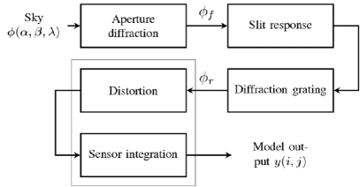
Figure 1: Block diagram of the direct model for one acquisition: from a continuously defined sky $\phi$ to a discrete output ${\mathb{y}}$ describing the data. The flux $\phi_{f}$ is a convolution of the flux $\phi$ and the PSF of the primary miror. $\phi_{f}$ is truncated by a rectangular slit and is dispersed by the gratting. Finally, the sensor provide a discrete output ${\mathb{y}}$.

II-A Aperture diffraction

Under some hypotheses, the propagation of a light wave which passes through an aperture is determined by Fresnel diffraction [15] and the result in the focal plane is a convolution of the input flux $\phi$ with the Point Spread Function (PSF) $h_{a}$ illustrated in Fig. 2 for a circular aperture. This PSF, which is a low pass filter, has a width proportional to the wavelength of the incident flux. For a circular aperture, it can be written:

$$h_{a}(\alpha,\beta,\lambda)=A\left[2\frac{J_{1}(\pi D\sqrt{\alpha^{2}+\beta^{2}}/\lambda)}{\pi D\sqrt{\alpha^{2}+\beta^{2}}/\lambda}\right]^{2}$$ (1)

where $J_{1}$ is the first order Bessel function of the first kind, $A$ is an amplitude factor and $D$ is the diameter of the mirror.

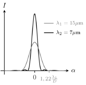
Figure 2: Profile of an Airy disk (PSF for a circular aperture) for two wavelengths.

The flux in the focal plane, $\phi_{f}$, is written in integral form:

$$\phi_{f}(\alpha^{\prime},\beta^{\prime},\lambda)=\iint_{\alpha,\beta}\phi(\alpha,\beta,\lambda)\,h_{a}(\alpha-\alpha^{\prime},\beta-\beta^{\prime},\lambda)\,{\mathrm{d}}\alpha\,{\mathrm{d}}\beta$$ (2)

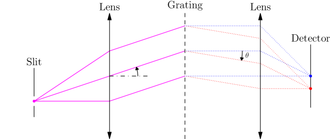
Figure 3: Optical scheme of IRS instrument: the slit is on the focal plan of the telescope Spitzer. The gratting disperses the light and the detector collectes the dispersed flux

II-B Slit and diffraction grating

Slit

Ideally, the slit and grating enable the dispersion of the wavelengths in spatial dimension $\beta$ previously “suppressed” by the slit (see Fig. 3). In practice, the slit cannot be infinitely narrow because the flux would be zero. The slit thus has a width $\gamma$ of about two pixels.

Diffraction grating

Ideally, the grating gives a diffracted wave with an output angle $\theta$ linearly dependent on the wavelength $\lambda$ (see Fig. 3). In a more accurate model, the dependencies become more complex. Let us introduce a variable $u$ in order to define an invariant response $h_{r}$ of the system [16].

$$u=\frac{\sin\theta-\sin\beta^{\prime}}{\lambda}\approx\frac{\sin\theta-\beta^{\prime}}{\lambda}$$ (3)

where $\beta^{\prime}$ is the angle of incidence of the wave on the grating , and $|\beta^{\prime}|\leq\gamma/2$ where $\gamma$ is the angular slit width (5.6 arcseconds). The response of the grating centred on mode $m$ ($m=0,1,\dots$) can, with some approximations, be written as the square of a cardinal sine centred on $m/a$ [16].

$$h_{r}(\theta,\beta^{\prime},\lambda)=B\,{\mathrm{sinc}}\,^{2}\left(\pi L(u-m/a)\right)$$ (4)

where $L$ is the width of the grating and $a$ the grid step (distance between two grooves). This response centred on the first mode ($m=1$) is plotted in Fig. 4.

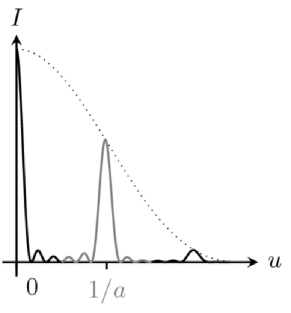
Figure 4: Diffraction grating response. The grey curve corresponds to the first mode. In reality, the response width is smaller.

As the flux is an incoherent light source, the expression for the signal at the output of the grating is written in the form of an integral over $\beta^{\prime}$ and $\lambda$:

$$\phi_{r}(\alpha^{\prime},\theta)=\int_{\lambda}\int_{|\beta^{\prime}|\leq\gamma/2}\phi_{f}(\alpha^{\prime},\beta^{\prime},\lambda)h_{r}(\beta^{\prime},\lambda,\theta){\mathrm{d}}\beta^{\prime}{\mathrm{d}}\lambda$$ (5)

where $l$ is the slit width.

II-C Sensor integration

Once the flux has passed through the grating and the wavelengths have been dispersed according to $\theta$, the light flux is focused on the sensor composed of square detectors. The sensor is simply modelled by integrating the flux $\phi_{r}$ on square areas of side $d$. The flux is integrated along the direction $\alpha$, which is not modified by the diffraction grating, and the dimension $\theta$, a combination of $\beta$ and $\lambda$, to obtain the discrete values

$$y(i,j)=\int_{id}^{(i+1)d}\int_{jd+e_{ij}^{1}}^{(j+1)d+e_{ij}^{2}}\phi_{r}(\alpha^{\prime},\theta){\mathrm{d}}\alpha^{\prime}{\mathrm{d}}\theta.$$ (6)

The integration limits are modified by the terms $e_{ij}^{n}$ in order to take into account the data distortion as illustrated in Fig. 5.

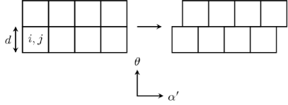
Figure 5: Modelling the distortion: sensor integration limits are shifted according to the dimensions $\alpha^{\prime}$.

II-D Scanning procedure of the sky

In a direction parallel to the slit width a scanning procedure (illustrated Fig. 6) is applied. This scanning procedure is composed of $Q$ acquisitions. Between the first and the $q^{th}$ acquisitions, the instrument is moved by $\Delta_{\alpha}(q)$ (resp. $\Delta_{\beta}(q)$) in the direction $\alpha$ (resp. $\beta$). To taking into account the motion of the instrument, we substitue $\phi(\alpha,\beta,\lambda)$ for $\phi(\alpha-\Delta_{\alpha}(q),\beta-\Delta_{\beta}(q),\lambda)$ in the previous equations. In practice, we fix the $\alpha$ axis in the direction of the slit and the $\beta$ axis perpendicular to the slit (see Fig. 6). In consequence, $\Delta_{\alpha}(q)$ is equal to zero.

II-E Complete model

By combining expression (1), (2), (5),(4) and (6), we obtain a continuous direct model in the form

$$y(i,j,q)=\mathcal{A}\int_{id}^{(i+1)d}\int_{jd+e_{ij}^{1}}^{(j+1)d+e_{ij}^{2}}\int_{\lambda}\int_{|\beta^{\prime}|\leq\gamma/2}\\ \int_{\alpha}\int_{\beta}\phi(\alpha-\Delta_{\alpha}(q),\beta-\Delta_{\beta}(q),\lambda)h_{a}(\alpha-\alpha^{\prime},\beta-\beta^{\prime},\lambda){\mathrm{d}}\alpha{\mathrm{d}}\beta\\ h_{r}(\theta,\beta^{\prime},\lambda){\mathrm{d}}\beta^{\prime}{\mathrm{d}}\lambda{\mathrm{d}}\alpha^{\prime}{\mathrm{d}}\theta$$ (7)

where $\mathcal{A}$ is a scale factor.

The equation (7) can rewritten:

$$y(i,j,q)=\int_{\alpha}\int_{\beta}\int_{\lambda}\phi(\alpha,\beta,\lambda)h_{tot}^{i,j,q}(\alpha,\beta,\lambda){\mathrm{d}}\alpha{\mathrm{d}}\beta{\mathrm{d}}\lambda$$ (8)

with

$$h_{tot}^{i,j,q}(\alpha,\beta,\lambda)=\mathcal{A}\int_{id}^{(i+1)d}\int_{jd+e_{ij}^{1}}^{(j+1)d+e_{ij}^{2}}\int_{-\gamma/2}^{\gamma/2}\\ h_{a}(\alpha-\alpha^{\prime}-\Delta_{\alpha}(q),\beta-\beta^{\prime}-\Delta_{\beta}(q),\lambda)h_{r}(\theta,\beta^{\prime},\lambda){\mathrm{d}}\alpha^{\prime}{\mathrm{d}}\theta{\mathrm{d}}\beta^{\prime}$$ (9)

We have been developed a model relying the continuous sky $\phi(\alpha,\beta,\lambda)$ and discrete data ${\mathb{y}}$. Our model is linear not-shift-invariant, because the aperture response and the grating response depend on the wavelength.

III Decomposition over a family and Gaussian approximation

In the previous part, we have seen that obtaining the output from the model requires the six integrals of equation (7) to be calculated. The estimation of $\hat{\phi}$ in $L^{2}(\mathbb{R})$ by inversion of this model is quite tricky, so we prefer to decompose the object over a family of functions. As we can see in the introduction, a lot of such decomposition functions can be used. The most traditional are Fourier bases, wavelets, cardinal sines, splines and pixel indicators. The choice does not have any great influence on the final result if the continuous object is decomposed over a sufficiently large number of functions. We therefore chose our decomposition functions in such a way as to reduce the computing time for the instrument model. First, we chose the $\alpha$ axis in the direction of the slit and the $\beta$ axis perpendicular to the slit (see Fig. 6). Second, we have two spatial variables $(\alpha,\beta)$ and one spectral variable $\lambda$, so to simplify the calculus, we chose decomposition functions that are separable into $(\alpha,\beta)$ and $\lambda$. Thrid, the object is convolved by the response of the optics, which has circular symmetry. So we choose functions possessing the same circular symmetry in order to make this calculation explicit. Finally, the slit and the grating have an impact in the $\beta$ direction only (5), which motivates us to choose functions that are separable into $\alpha$ and $\beta$. These considerations led us to choose Gaussian functions along the spatial directions. Finally the complexity of the $\lambda$ dependence encouraged us to choose Dirac impulses for the spectral direction.

III-A Decomposition over a family of Gaussian functions

The flux $\phi$ is a continous function decomposed over a family of separable functions:

$$\phi(\alpha,\beta,\lambda) = \sum_{k}\sum_{l}\sum_{p}x(k,l,p)$$ (10)

$$\Pi(\alpha-kT_{\alpha})\,\Phi(\beta-lT_{\beta})\,\Gamma(\lambda-pT_{\lambda})$$

$$= \sum_{k}\sum_{l}\sum_{p}x(k,l,p)\Psi_{k,l,p}(\alpha,\beta,\lambda)$$

where $x(k,l,p)$ are the decomposition coefficients, $T_{\alpha}$, $T_{\beta}$ and $T_{\lambda}$ are the sampling steps, and with:

$$\Pi(\alpha)\Phi(\beta) = \frac{1}{2\pi\sigma^{2}}\exp\left(-\frac{1}{2}\frac{\alpha^{2}+\beta^{2}}{\sigma^{2}}\right)$$ (11)

$$\Gamma(\lambda) = \delta(\lambda)$$ (12)

With such decomposition, the inverse problem becomes one of estimating a finite number of coefficients $x(k,l,p)$ from discrete data $y(i,j,q)$. By combining equations (8) and (10), we obtain:

$$y(i,j,q)=\sum_{k}\sum_{l}\sum_{p}x(k,l,p)\int_{\alpha}\int_{\beta}\int_{\lambda}\Psi_{k,l,p}(\alpha,\beta,\lambda)\\ h_{tot}^{i,j,q}(\alpha,\beta,\lambda){\mathrm{d}}\alpha{\mathrm{d}}\beta{\mathrm{d}}\lambda$$ (13)

If the $y(i,j,q)$ and $x(k,l,p)$ are gathered in vectors ${\mathb{y}}$ and ${\mathb{x}}$ respectively, the equation (13) can be formalized as a vector matrix product.

$${\mathb{y}}={\mathb{H}}{\mathb{x}}$$ (14)

with each component of the matrix ${\mathb{H}}$ is calculated using the integral part of the equation (13). The $n(k,l,p)$-th column of matrix ${\mathb{H}}$ constitutes the output when the model is used with the $n$-th decomposition function ($\Psi_{k,l,p}$). The model output for $\Psi_{k,l,p}$ is calculated in the next two sections.

III-B Impulse responses approximated by Gaussian functions

III-B1 Approximation of the PSF

Equation (2) comes down to convolutions of a squared Bessel function and Gaussians. This integral is not explicit and, in order to carry out the calculations, the PSF is approximated by a Gaussian

$$\tilde{h}_{a}(\alpha,\beta,\lambda)=\frac{1}{2\pi\sigma_{\lambda}^{2}}\exp\left(-\frac{1}{2}\frac{\alpha^{2}+\beta^{2}}{\sigma_{\lambda}^{2}}\right)$$

with a standard deviation $\sigma_{\lambda}$ depending on the wavelength. Indeed, the Bessel functions cross zero at the first time in $1.22{\lambda/D}$. $\sigma_{\lambda}$ is determined numerically by minimizing the quadratic error between the Gaussian kernel and the squared Bessel function, which gives for our instrument $\sigma_{\lambda}\approx\lambda/2$. The relative quadratic error $err_{L2}={\|\text{Bessel}-\text{Gaussian}\|^{2}_{2}\;/\;\|\text{Bessel}\|^{2}_{2}}$ is equal to $0.15\%$ for our instrument. If we caculate the relative absolute error $err_{L1}={\|\text{Bessel}-\text{Gaussian}\|_{1}\;/\;\|\text{Bessel}\|_{1}}$, we obtain 5 %. We can conclude that most of the energy of the squared bessel function is localized in the primary lobe. Another advantage of using the Gaussian approximation is that the convolution kernel is separable into $\alpha$ and $\beta$. Finally, the result of the convolution of two Gaussian functions is a standard one and is also a Gaussian:

$$\tilde{h}_{a}(\alpha,\beta,\lambda)\star\Pi(\alpha)\Phi(\beta)=\frac{1}{2\pi(\sigma_{\lambda}^{2}+\sigma^{2})}\exp\left(-\frac{\alpha^{\prime 2}+\beta^{\prime 2}}{2(\sigma_{\lambda}^{2}+\sigma^{2})}\right)$$ (15)

III-B2 Approximation of the grating response

The presence of the slit means that integral (5) is bounded over $\beta^{\prime}$ and is not easily calculable. Since the preceding expressions use Gaussian functions, we approximate the squared cardinal sine by a Gaussian to make the calculations easier:

$$\text{sinc}^{2}\left(\pi L\left(\frac{\sin\theta-\beta^{\prime}}{\lambda}-\frac{m}{a}\right)\right)\approx\\ \frac{1}{\sqrt{2\pi}\lambda\sigma_{s}}\exp\left(-\frac{1}{2}\frac{(\frac{\sin\theta-\beta^{\prime}}{\lambda}-\frac{m}{a})^{2}}{\sigma_{s}^{2}}\right)$$ (16)

$\sigma_{s}$ is determined numerically by minimizing the quadratic error between the Gaussian kernel and the squared cardinal sine, which gives for our instrument $\sigma_{s}\approx 25.5\;\mathrm{m}^{-1}$. The relative errors made are larger than the bessel case ($err_{L2}=0.43\%,err_{L1}=10.7\%$), but this Gaussian approximation of the grating response allows the flux $\phi_{r}$ coming out of the grating to be known explicitly.

The error introduced here is larger than for the Gaussian approximation of the PSF described in the previous section. However, our goal is to have a good model of the spatial dimension of the array. Furthermore, with respect to the current method, the fact of taking the response of the grating into consideration, even as an approximation, is already a strong improvement.

$$\phi_{r}(\alpha^{\prime},\theta) = \int_{\lambda}\int_{-\gamma/2}^{\gamma/2}\int_{\alpha}\int_{\beta}\Pi(\alpha-\alpha_{k})\Phi(\beta-\beta_{l}-\Delta_{\beta}(q))$$ (17)

$$\Gamma(\lambda-\lambda_{p})\tilde{h}_{a}(\alpha-\alpha^{\prime},\beta-\beta^{\prime},\lambda)\tilde{h}_{r}(\theta,\beta^{\prime},\lambda)$$

$${\mathrm{d}}\alpha{\mathrm{d}}\beta{\mathrm{d}}\beta^{\prime}{\mathrm{d}}\lambda$$

$$= \mathcal{A}\exp\left(-\frac{(\alpha^{\prime}-\alpha_{k})^{2}}{2(\sigma_{\lambda}^{2}+\sigma^{2})}\right)\exp\left(-\frac{(\sin\theta-\nu)^{2}}{2\Sigma^{2}}\right)$$

$$\times\left[\mbox{erf}\left(\frac{\gamma/2-\mu}{\Sigma^{\prime}\sqrt{2}}\right)-\mbox{erf}\left(\frac{-\gamma/2-\mu}{\Sigma^{\prime}\sqrt{2}}\right)\right]$$

with

$$\left\{\begin{array}[]{lcc}\mathcal{A}&=&\displaystyle\frac{1}{4\pi}\sqrt{\frac{1}{(\sigma_{\lambda}^{2}+\sigma^{2})(\sigma_{\lambda}^{2}+\sigma^{2}+\lambda_{p}^{2}\sigma_{s}^{2})}}\\ \Sigma^{2}&=&(\sigma_{\lambda}^{2}+\sigma^{2})+\lambda_{p}^{2}\sigma_{s}^{2}\\ \nu&=&\displaystyle\frac{m\lambda_{p}}{a}+\beta_{l}+\Delta_{\beta}(q)\\ \Sigma^{\prime}&=&\displaystyle\frac{\sqrt{\sigma_{\lambda}^{2}+\sigma^{2}}\lambda_{p}\sigma_{s}}{\sqrt{\sigma_{\lambda}^{2}+\sigma^{2}+\lambda_{p}^{2}\sigma_{s}^{2}}}\\ \mu&=&\displaystyle\frac{\left(\sin\theta-\frac{m\lambda_{p}}{a}\right)(\sigma_{\lambda}^{2}+\sigma^{2})}{(\sigma_{\lambda}^{2}+\sigma^{2})+\lambda_{p}^{2}\sigma_{s}^{2}}\\ \mbox{erf}(a)&=&\displaystyle\frac{2}{\sqrt{\pi}}\int_{0}^{a}e^{-t^{2}}{\mathrm{d}}t\end{array}\right.$$

In equation (17), it can be seen that $\phi_{r}$ is separable into $\alpha^{\prime}$ and $\theta$. Let us introduce the functions $f$ and $g$ such that:

$$\phi_{r}(\alpha^{\prime},\theta)=\mathcal{A}f(\alpha^{\prime})g(\theta)$$ (18)

III-C Sensor integration

First, we calculate the sensor integration in the $\alpha^{\prime}$ direction.

$$\int_{jd+e_{ij}^{1}}^{(j+1)d+e_{ij}^{2}}f(\alpha^{\prime}){\mathrm{d}}\alpha^{\prime}=\\ \mathcal{K}\left[\mbox{erf}\left(\frac{(j+1)d+e^{2}_{ij}-\alpha_{k}}{\sqrt{2(\sigma_{\lambda}^{2}+\sigma^{2})}}\right)-\mbox{erf}\left(\frac{jd+e^{1}_{ij}-\alpha_{k}}{\sqrt{2(\sigma_{\lambda}^{2}+\sigma^{2})}}\right)\right]$$ (19)

with $\mathcal{K}=\sqrt{\pi(\sigma_{\lambda}^{2}+\sigma^{2})/2}$

The integral of $g$ is calculated numerically as the presence of erf functions in equation (17) does not allow analytical calculations.

We obtain the expression for the $n$-th column of matrix ${\mathb{H}}$, which now contains only a single integral:

$$y(i,j,q)=\mathcal{AK}\int_{id}^{(i+1)d}g(\theta){\mathrm{d}}\theta\\ \times\left[\mbox{erf}\left(\frac{(j+1)d+e^{2}_{ij}-\alpha_{k}}{\sqrt{2(\sigma_{\lambda}^{2}+\sigma^{2})}}\right)-\mbox{erf}\left(\frac{jd+e^{1}_{ij}-\alpha_{k}}{\sqrt{2(\sigma_{\lambda}^{2}+\sigma^{2})}}\right)\right]$$ (20)

Using expression (20), the elements of matrix ${\mathb{H}}$ are pre-computed relatively rapidly. Thanks to the sparsity of the matrix ${\mathb{H}}$ to calculate the model output of Eq. (14).

IV Inversion

The previous sections build the relationship (14) between the object coefficients and the data: it describes a complex instrumental model but remains linear. The problem of input (sky) reconstruction is a typical inverse problem and the literarure on the suject is abundant.

The proposed inversion method resorts to linear processing. It is based on conventional approaches described in books such [17, 18] or more recently [19]. In this framework, the reader may also consider [20, 21] for inversion based on specific decomposition. These methods rely on a quadratic criterion

$$J({\mathb{x}})=||{\mathb{y}}-{\mathb{H}}{\mathb{x}}||^{2}+\mu_{\alpha\beta}||{\mathb{D}}_{\alpha\beta}{\mathb{x}}||^{2}+\mu_{\lambda}||{\mathb{D}}_{\lambda}{\mathb{x}}||^{2}\,.$$ (21)

It involves a least squares term and two penality terms concerning the differences between neighbouring coefficients: one for the two spatial dimensions and one for the spectral dimension. They are weighted by $\mu_{\alpha\beta}$ and $\mu_{\lambda}$, respectively. The estimate $\hat{\mathb{x}}$ is chosen as the minimizer of this criterion. It is thus explicit and linear with respect to the data:

$$\hat{\mathb{x}}=\left({\mathb{H}}^{\mathrm{t}}{\mathb{H}}+\mu_{\alpha\beta}{\mathb{D}}_{\alpha\beta}^{\mathrm{t}}{\mathb{D}}_{\alpha\beta}+\mu_{\lambda}{\mathb{D}}_{\lambda}^{\mathrm{t}}{\mathb{D}}_{\lambda}\right)^{-1}{\mathb{H}}^{\mathrm{t}}{\mathb{y}}$$ (22)

and depends on the two regularization parameters $\mu_{\alpha\beta}$ and $\mu_{\lambda}$.

Remark 1

—  This estimator can be interpreted in a Bayesian framework [22] based on Gaussian models for the errors and the object. As far as the errors are concerned, the model is a white noise. As far as the object is concerned, the model is correlated and the inverse of the correlation matrix is proportional to $\mu_{\alpha\beta}{\mathb{D}}_{\alpha\beta}^{\mathrm{t}}{\mathb{D}}_{\alpha\beta}+\mu_{\lambda}{\mathb{D}}_{\lambda}^{\mathrm{t}}{\mathb{D}}_{\lambda}$, i.e., it is a Gauss markov field. In this framework, the estimate maximizes the a posteriori law.

Remark 2

—  Many works in the field of over-resolved reconstruction concern edge preserving priors [23, 11, 7, 24, Humblot06, 12]. In our application here, smooth interstellar dust clouds are under study, so preservation of edges is not appropriate. For the sake of simplicity of implementation, we chose a Gaussian object prior.

The minimizer $\hat{\mathb{x}}$ given by relation (22) is explicit but, in practice, it cannot be calculated on standard computers, because the matrix to be inverted is too large. The solution $\hat{\mathb{x}}$ is therefore computed by a numerical optimization algorithm. Practically, the optimization relies on a standard gradient descent algorithm [25, 26]. More precisely, the direction descent is a approximate conjugate gradient direction [27] and the optimal step of descent is used. Finally, we initialise the method with zero (${\mathb{x}}=0$).

V Results

As we have presented in part III the $\alpha$ and $\beta$ axis are fix (see Fig. 6, right). The real data is composed of 23 acquisitions having a spatial dimension $\alpha^{\prime}$ and a spectral dimension $\theta$ of wavelength between 7.4 and 15.3 $\mu\mathrm{m}$ (each acquisition is an image composed of $38\times 128$ detector cells, see Fig. 6, left). Between two acquisitions, the instrument is moved by half a slit width in the $\beta$ direction. Fig. 6, right, shows the scanning procedure applied to the Horsehead nebula [28].

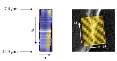
Figure 6: Acquisition. The left-hand image represents the data acquired for one pointing position: the vertical axis shows the spectral dimension $\theta$ and the horizontal axis is the spatial dimension $\alpha^{\prime}$. The slit is represented schematically by a rectangle in the middle. The right-hand image illustrates the scanning strategy in the $\beta$ direction.

Our results (Fig. 8, solid line on Fig. 9 and Fig. 10) can be compared with those obtained with the conventional processing (Fig. 8, dotted line on Fig. 9 and Fig. 10). For the conventional processing (described in Compiègne et al. 2007 [28]) an image of the slit is simply extracted for each wavelength from the data taken after each acquisition (e.g. left panel of Fig. 6) and projected and co-added on the output sky image, without any description of the instrument properties.

V-A Simulated data

In our first experiment, we reconstruct data simulated using our direct model. We choose an object with the same spatial morphology and the same spectral content as the Horsehead nebula (see Fig. 8). However, in order to tune the regularization coefficient, we perform a large number of reconstructions. Thus, we need to simulate a problem smaller than in our real case. The data are composed of 14 acquisitions, and the virtual detector contained $18\times 40$ pixels. We choose to reconstruct a volume with 15870 gaussians distributed on a cartesian grid $23\times 23\times 30$. Finally, we add to the output of the model a white Gaussian noise with the same variance as the real data.

The results contain a set of 30 images (see Fig. 7). Fig. 8 and solid line on Fig.9 illustrate our result for one wavelength (8.27 $\mu m$) and one pixel, respectively. The image computed with our method (Fig. 8) appears comparable to the true image (Fig. 8), while the image computed with the conventional processing (Fig. 8) is smoother. A comparison of solid line and dotted line in Fig. 9 clearly also shows that our method provides a spectrum comparable to the true spectrum, while the peaks obtained with the conventional processing are too broad.

Our sky estimation depends on the regularization coefficients $\mu_{\alpha\beta}$ and $\mu_{\lambda}$. We tune this parameters by minimizing numerically the quadratic error between the estimated object and the real object were selected. In this experiment we obtain $\mu_{\alpha\beta}=0.01,\;\mu_{\lambda}=0.005$.

Figure 7: Set of 30 images of our reconstruction from simulated data. Each image corresponds to one wavelength for 7.4 to 9.2 $\mu m$ with a step of 0.062 $\mu m$.

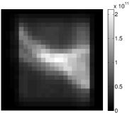
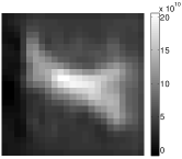
Figure 8: Image at $\lambda=8.27\,\mu\mathrm{m}$:, (a) simulated sky, (b) image estimated by our method, (c) image estimated by a conventional method.

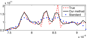
Figure 9: Spectrum of a pixel. The curves abscissa is the wavelenght in meters: solid line: simulated sky, dashed line: our method, dotted line: conventional method.

V-B Real data

Eeal data contain 23 acquisitions composed of $38\times 128$ values. To obtain a over-resolved reconstruction, we describe our volume with 587264 gaussians destributes on a cartesian grid $74\times 62\times 128$. The spatial $(\alpha,\beta)$ sampling step is equal to a quater slit width, and the spectral dimension is uniformly sampled between the wavelength 7.4 and 15.3 $\mu\mathrm{m}$. The reconstruction is computed after setting the regularization coefficients $\mu_{\alpha\beta}$ and $\mu_{\lambda}$ empirically. Too low a value for these coefficients produces an unstable method and a quasi explosive reconstruction. Too high a value produces images that are visibly too smooth. A compromise found by trial and error led us to $\mu_{\alpha\beta}=0.3$ and $\mu_{\lambda}=0.7$. The ratio between $\mu_{\alpha\beta}$ and $\mu_{\lambda}$ is also based on our simulation. However, we cannot compare the regularization coefficients between the simulated and the real case, since the size of the problem modifies the weigth of the norm in the Eq. (21). Pratically, we take large value for the regularization coefficients, and we gradually reduce the value up that we are seeing noise.

Our results (Fig. 10 and 11) can be compared with those obtained with (Fig. 10 and 11, from [28]). A comparison of Fig. 10 and 10 clearly shows that our approach provides more resolved images that bring out more structures than the conventional approach. Note, in particular, the separation of the two filaments on the left part of the Fig. 10 obtained with our method, which remains invisible after conventional processing. For comparison, Fig. 10 shows the same object observed with the Infrared Array Camera (IRAC) of the Spitzer Space Telescope which has a better native resolution since it observes at a shorter wavelength (4.5 $\mu\mathrm{m}$). Here the same structures are observed, providing a strong argument in favour of the reality of the results provided by our method.

A more precise analysis is done in section V-C. It provides a quantitative evaluation of the resolution.

Finally, the spectra reconstructed by our method (Fig. 11) have a resolution slightly better than the one reconstructed by the conventional method (Fig. 11). The peaks characterizing the observed matter (gas and dust) are well positioned, narrower and with a greater amplitude. However, ringing effects appear at the bases of the strongest peaks (Fig. 11). They could be explained by an over-evaluation of the width $\sigma_{s}$ of the response of the grating, or by the gaussian approximation.

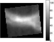
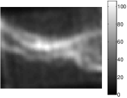
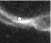
Figure 10: Reconstruction of a sky $\phi$ representing the Horsehead nebula: (a) image estimated at 11.37 $\mu\mathrm{m}$ by the conventional method (b) image estimated at 11.37 $\mu\mathrm{m}$ by our method, (c) image obtained with the Infrared Array Camera IRAC on board the Spitzer Space Telescope having better resolution at 4.5 $\mu\mathrm{m}$.

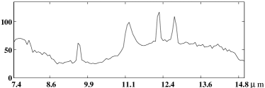
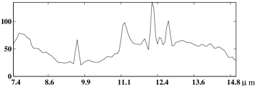
Figure 11: Spectrum of the center point of the Fig. 10: (a) spectrum estimated with the conventional method (b) spectrum estimated with our method.

V-C Study of resolving power of our approach

This part is devoted to numerical quantification of the gain in angular resolution provided with our method, using the Rayleigh criterion, which is frequently used by astrophysicists: for the smaller resolvable detail, the first minimum of the image of one point source coincides with the maximum of another. In practice, two point sources with the same intensity and a flat strectrum are considered to be separated if the minimal flux between the two peaks is lower than 0.9 times the flux at the peak positions. The resolution is studied in the $\beta$ direction only as this is the direction in which the subslit scan is performed.

Two point sources are injected, at positions $\beta_{1}$ and $\beta_{2}$, respectively (see Fig. 13, top). The corresponding data are simulated, and the reconstruction $\hat{\phi}(\beta)$ is performed. As explained above, the two point sources are considered to be separated if $\hat{\phi}(\left[\beta_{1}+\beta_{2}\right]/2)\leq 0.9\times\hat{\phi}(\beta_{1})$. The resolution is defined as the difference $\delta=\beta_{2}-\beta_{1}$ at which the two point sources start to be separated.

Point sources are simulated for a set of differences $\delta$ between 2.4 and 5.4 arcseconds and simulations are performed in the configuration of the real data (signal to noise ratio, energy of the data). Moreover, we use the regularization parameters $\mu_{\alpha\beta}$ and $\mu_{\lambda}$ determined in section V-A. A number of reconstructions has been obtained. The ratio between the values of the reconstructed function at $\beta_{1}$ and $(\beta_{1}+\beta_{2})/2$ is calculated as a function of the difference $\delta$ between the two peaks. Results are shown in Fig. 12.

The computed resolution is 3.4 arcseconds (see Fig. 12(a)) and 5 arcseconds (see Fig. 12(b)) for our method and the conventional method, respectively. Fig. 13 illustrates this gain in angular resolution. In the left column on Fig. 13 ($\delta=3.4$) corresponds to the limit of resolution of our method. In this case, the peak is not separated with the conventional method (Fig. 13 (d)). In the middle column on Fig. 13, our algorithm clearly separates the peak (Fig. 13(h)) and not the conventional method (Fig. 13(e)). In the right column, we observe a stain with our method is smaller than the conventional method. Our method increases the resolution by a factor 1.5.

(a)

(b)

Figure 12: Resolution of our method: the curve represents the ratio of the intensity at one peak to the intensity between the two peaks as a function of the distance between the peaks in arcseconds. The resolution is read at crossing of this curve and the dotted line (the ratio is 0.9). (a) Results obtained with our method. (b) Results obtained with the conventional method

.

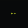
(a)	(b)	(c)
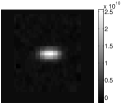
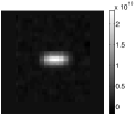
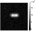
(d)	(e)	(f)
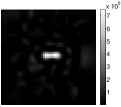
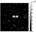
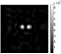
(g)	(h)	(i)

Figure 13: Two peaks reconstruction for different $\delta$ : (a-c) Visualisation of the peaks position for $\delta=3.4$, 4 and 5.4 arcsecond resp., (d-f) reconstruction with the conventional method for $\delta=3.4$, 4 and 5.4 arcsecond resp., (g-i) reconstruction with our over-resolution method for $\delta=3.4$, 4 and 5.4 arcsecond respectively.

VI Conclusions

We have developed an original method for reconstructing the over-resolved 3D sky from data provided by the IRS instrument. This method is based on:

1. a continuous variable model of the instrument based on a precise integral physical description,

2. a decomposition of the continuous variable object over a family of Gaussian functions, which results in a linear, semi-parametric relationship,

3. an inversion in the framework of deterministic regularization based on a quadratic criterion minimized by a gradient algorithm.

The first results on real data show that we are able to evidence spatial structures not detectable using conventional methods. The spatial resolution is improved by a factor 1.5. This factor should increase using data with a motion between two acquisitions smaller than the half a slit width.

In the future, we plan to design highly efficient processing tools using our approach in particular for the systematic processing of the data which will be taken with the next generation of infrared to milimeter space observatory (Herschel, Planck, …).

Thomas Rodet was born in Lyon, France, in 1976. He received the Doctorat degree at Institut National Polytechnique de Grenoble, France, in 2002. He is presently assistant professor in the Département de Physique at Université Paris-Sud 11 and researcher with the Laboratoire des Signaux et Systèmes (CNRS - Supélec - UPS). He is interested in tomography methods and Bayesian methods for inverse problems in astrophisical problems (inversion of data taken from space observatory: Spitzer, Herschel, SoHO, STEREO).

François Orieux was born in Angers, France, in 1981. He graduated from the École Supérieure d’Électronique de l’Ouest in 2006 and obtain the M. S. degree from the University of Rennes 1. He currently pursuing the Ph. D. degree at the Université Paris-Sud 11. His research interests are statistical image processing and Bayesian methods for inverse problems.

Jean-François Giovannelli was born in Béziers, France, in 1966. He graduated from the École Nationale Supérieure de l’Électronique et de ses Applications in 1990. He received the Doctorat degree in physics at Université Paris-Sud, Orsay, France, in 1995. He is presently assistant professor in the Département de Physique at Université Paris-Sud and researcher with the Laboratoire des Signaux et Systèmes (CNRS - Supélec - UPS). He is interested in regularization and Bayesian methods for inverse problems in signal and image processing. Application fields essentially concern astronomical, medical and geophysical imaging.

Alain Abergel was born in Paris, France, in 1959. He received the Doctorat degree in astrophysics at the Paris 6 University, France, in 1987, and is presently Professor in Physics and Astronomy at the Paris-Sud University. He is interested in the interstellar medium of galaxies, and uses data taken from long wavelength space observatories (IRAS, COBE, ISO, Spitzer, … ). He is Co-investigator for the Spectral and Photometric Imaging Receiver (SPIRE) instrument on-board the European Space Agency’s Herschel Space Observatory.

References

- [1] J. R. Houck et al., “The infrared spectrograph (IRS) on the Spitzer space telescope,” ApJS, vol. 154, pp. 18–24, September 2004.
- [2] R. M. Lewitt, “Multidimensional digital image representations using generalized Kaiser-Bessel window functions,” J. Opt. Soc. Am. A, vol. 7, no. 10, pp. 1834–1848, October 1990.
- [3] ——, “Alternative to voxels for image representation in iterative reconstruction algorithms,” Physics in Medicine and Biology, vol. 37, pp. 705–716, 1992.
- [4] S. Matej and R. M. Lewitt, “Practical considerations for 3-D image reconstruction using spherically symmetric volume elements,” IEEE Trans. Medical Imaging, vol. 15, pp. 68–78, January 1996.
- [5] A. Andreyev, M. Defrise, and C. Vanhove, “Pinhole SPECT reconstruction using blobs and resolution recovery,” IEEE Trans. Nuclear Sciences, vol. 53, pp. 2719–2728, October 2006.
- [6] S. C. Park, M. K. Park, and M. G. Kang, “Super-resolution image reconstruction: a technical overview,” IEEE Trans. Signal Processing Mag., pp. 21–36, May 2003.
- [7] M. Elad and A. Feuer, “Restoration of a single superresolution image from several blurred, noisy, and undersampled measured images,” IEEE Trans. Image Processing, vol. 6, no. 12, pp. 1646–1658, December 1997.
- [8] ——, “Superresolution restoration of an image sequence: Adaptive filtering approach,” IEEE Trans. Image Processing, vol. 8, no. 3, pp. 387–395, March 1999.
- [9] G. Rochefort, F. Champagnat, G. Le Besnerais, and J.-F. Giovannelli, “An improved observation model for super-resolution under affine motion,” IEEE Trans. Image Processing, vol. 15, no. 11, pp. 3325–3337, November 2006.
- [10] A. J. Patti, M. I. Sezan, and A. M. Tekalp, “Superresolution video reconstruction with arbitrary sampling lattices and nonzero aperture time,” IEEE Trans. Image Processing, vol. 6, no. 8, pp. 1064–76, August 1997.
- [11] R. C. Hardie, K. J. Barnard, and E. E. Armstrong, “Joint map registration and high-resolution image estimation using a sequence of undersampled images,” IEEE Trans. Image Processing, vol. 6, no. 12, pp. 1621–1633, December 1997.
- [12] N. A. Woods, N. P. Galatsanos, and A. K. Katsaggelos, “Stochastic methods for joint resgistration, restoration, and interpolation of multiple undersampled images,” IEEE Trans. Image Processing, vol. 15, no. 1, pp. 201–13, January 2006.
- [13] P. Vandewalle, L. Sbaiz, J. Vandewalle, and M. Vetterli, “Super-resolution from unregistrered and totally aliased signals using subspace methods,” IEEE Trans. Signal Processing, vol. 55, no. 7, pp. 3687–703, July 2007.
- [14] M. Piana, A. M. Massone, G. J. Hurford, M. Prato, A. G. Emslie, E. P. Kontar, and R. A. Schwartz, “Electron flux imaging of solar flares through regularized analysi of hard X-ray source visibilities,” The Astrophysical Journal, vol. 665, pp. 846–855, August 2007.
- [15] J. W. Goodman, Introduction à l’optique de Fourier et à l’holographie. Paris, France: Masson, 1972.
- [16] J.-P. Pérez, Optique, fondements et applications. Dunod, 2004.
- [17] A. Tikhonov and V. Arsenin, Solutions of Ill-Posed Problems. Washington, dc: Winston, 1977.
- [18] H. C. Andrews and B. R. Hunt, Digital Image Restoration. Englewood Cliffs, nj: Prentice-Hall, 1977.
- [19] J. Idier, Ed., Bayesian Approach to Inverse Problems. London: ISTE Ltd and John Wiley & Sons Inc., 2008.
- [20] M. Bertero, C. De Mol, and E. R. Pike, “Linear inverse problems with discrete data. I: General formulation and singular system analysis,” Inverse Problems, vol. 1, pp. 301–330, 1985.
- [21] ——, “Linear inverse problems with discrete data: II. stability and regularization,” Inverse Problems, vol. 4, p. 3, 1988.
- [22] G. Demoment, “Image reconstruction and restoration: Overview of common estimation structure and problems,” IEEE Trans. Acoust. Speech, Signal Processing, vol. assp-37, no. 12, pp. 2024–2036, December 1989.
- [23] R. R. Schultz and R. L. Stevenson, “Extraction of high-resolution frames from video sequences,” IEEE Trans. Image Processing, vol. 5, no. 6, pp. 996–1011, June 1996.
- [24] N. Nguyen, P. Milanfar, and G. Golub, “A computationally efficient superresolution image reconstruction algorithm,” IEEE Trans. Image Processing, vol. 10, no. 4, pp. 573–83, April 2001.
- [25] D. P. Bertsekas, Nonlinear programming, 2nd ed. Belmont, ma: Athena Scientific, 1999.
- [26] J. Nocedal and S. J. Wright, Numerical Optimization, ser. Series in Operations Research. New York: Springer Verlag, 2000.
- [27] E. Polak, Computational methods in optimization. New York, ny: Academic Press, 1971.
- [28] M. Compiègne, A. Abergel, L. Verstraete, W. T. Reach, E. Habart, J. D. Smith, F. Boulanger, and C. Joblin, “Aromatic emission from the ionised mane of the Horsehead nebula,” Astronomy & Astrophysics, vol. 471, pp. 205–212, 2007.