A consistent interpretation of the low temperature magneto-transport in graphite
using the Slonczewski–Weiss–McClure 3D band structure calculations

Abstract

Magnetotransport of natural graphite and highly oriented pyrolytic graphite (HOPG) has been measured at mK temperatures. Quantum oscillations for both electron and hole carriers are observed with orbital angular momentum quantum number up to $N\approx 90$. A remarkable agreement is obtained when comparing the data and the predictions of the Slonczewski–Weiss–McClure tight binding model for massive fermions. No evidence for Dirac fermions is observed in the transport data which is dominated by the crossing of the Landau bands at the Fermi level, corresponding to $dE/dk_{z}=0$, which occurs away from the $H$ point where Dirac fermions are expected.

Recently, massless Dirac fermions have been observed at the $K$ point of the Brillouin zone in graphene, a hexagonally arranged carbon monolayer with quite extraordinary properties K. S. Novoselov et al. (2005). Historically, graphene forms the starting point for the Slonczewski, Weiss and McClure (SWM) band structure calculations of graphite Slonczewski and Weiss (1958); McClure (1960). In graphite, the Bernal stacked graphene layers are weakly coupled with the form of the in-plane dispersion depending upon the momentum $k_{z}$ in the direction perpendicular to the layers. The carriers occupy a region along the $H-K-H$ edge of the hexagonal Brillouin zone. At the $K$ point ($k_{z}=0$), the dispersion of the electron pocket is parabolic (massive fermions), while at the $H$ point ($k_{z}=0.5$) the dispersion of the hole pocket is linear (massless Dirac fermions). A clear signature of Dirac fermions at the $H$ point of graphite has recently been reported using far-infrared magneto-absorption measurements M. Orlita et al. (2008). Such measurements probe the very close vicinity of the $H$ and $K$ points where there is a maximum in the joint density of states.

The SWM model, which provides a remarkably accurate description of the band structure, has been extensively tested using Shubnikov de Haas, de Haas van Alphen, thermopower and magneto-reflectance measurements to caliper the Fermi surface of graphite Soule (1958); Soule et al. (1964); Woollam (1970, 1971); Williamson et al. (1965); Schroeder et al. (1968). There are even reports of a charge density wave state above $B=22$ T Y. Iye et al. (1982); Timp et al. (1983); Iye and Dresselhaus (1985). However, the observation of massless carriers with a Dirac–like energy spectrum, using magneto-transport measurements Luk’yanchuk and Kopelevich (2004, 2006) remains controversial, since in the SWM model, the electrons and hole carriers at the Fermi level are both massive quasi–particles.

In this Letter, we report magneto-transport measurements of natural graphite at very low temperature ($T\approx 10$ mK). Due to the low temperatures used, the magneto-transport is much richer than previously published data Soule (1958); Soule et al. (1964); Woollam (1970, 1971); Williamson et al. (1965); Y. Iye et al. (1982); Timp et al. (1983); Iye and Dresselhaus (1985); Luk’yanchuk and Kopelevich (2004, 2006). Quantum oscillations are observed for both majority electrons and holes with orbital quantum number up to almost N=100. We show that these oscillations are fully consistent with the presence of majority electron and hole pockets within the three dimensional SWM band structure calculations for graphite. At high magnetic fields ($B>2$ T), a significant deviation from 1/B periodicity occurs due to the well documented movement of the Fermi energy as the quantum limit is approached Sugihara and Ono (1966); Woollam (1971). This seriously questions the validity of using the high field data to extract the phase of the Shubnikov de Haas oscillations, and hence the nature of the charge carriers Luk’yanchuk and Kopelevich (2006).

For the measurements mm-size pieces of natural graphite and highly oriented pyrolytic graphite (HOPG), a few hundred microns thick, where contacted in an approximate Hall-bar configuration using silver paint. The measurements were performed with the sample placed directly in the mixture of a He³/He⁴ dilution fridge, using an ac current of $\sim 10$ $\mu$A at $10.7$ Hz and conventional phase sensitive detection. The magnetic field was applied along the c–axis of the sample.

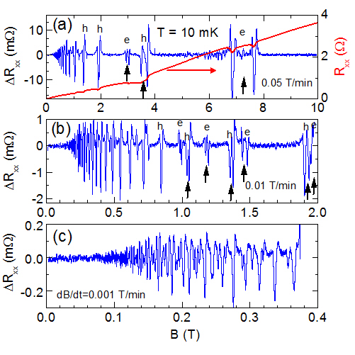
Figure 1: (color online) (a) Right axis: Resistance $R_{xx}$ versus B measured at $T=10$ mK for natural graphite. (a-c) Left axis: Background removed data $\Delta R_{xx}$ showing quantum oscillations measured over different magnetic field regions. The high field electron (e) and hole (h) features are indicated. The vertical arrows indicate spin split electron and hole features.

Typical low temperature data for $R_{xx}$ $\mathrm{(\Omega)}$ as a function of the magnetic field from $B=0-10$ T for natural graphite, is shown in Fig. 1(a). $R_{xx}(B)$ increases roughly linearly with the magnetic field and at $B=10$ T, it is about three orders of magnitude larger than the zero-field value McClure and Spry (1968); Abrikosov (1999); X. Du et al. (2005); J. C. González et al. (2007). In addition, quantum oscillations are superimposed on the large magneto-resistance background. These oscillations, can be better seen in the background removed data $\Delta R_{xx}$ plotted in Fig. 1(a-c) for successively slower sweeps in order to reveal the quantum oscillations in the different magnetic field regions. The background can either be removed by subtracting a smoothed (moving window average) data curve or by numerically calculating the second derivative $d^{2}R/dB^{2}$. Both techniques give similar results and here we use averaging to remove the background. As the oscillations are periodic in $1/B$, the optimal number of points used in the averaging depends upon the magnetic field region. For this reason, the amplitudes of the oscillations in Fig. 1(a-c) should not be compared, as different averaging was used to remove the background. HOPG (not shown) presents almost identical oscillations, with very slightly different frequencies, and a significantly reduced amplitude M. Orlita et al. (2008). For this reason we concentrate here on the data for natural graphite.

In the $\Delta R_{xx}(B)$ data shown in Fig. 1 two series of oscillations can be distinguished. The oscillations start at a magnetic field $B\approx 0.1$ T, and spin splitting of the features (indicated by arrows) is observed for magnetic fields $B>1$ T, compared to previous work Woollam (1970) in which spin-splitting was only observed for the three last features at magnetic fields $B>2$ T. The electronic g-factor $g_{s}$ can be estimated from the magnetic fields at which spin splitting occurs, ($B_{z}\sim 1$ T), and at which the Shubnikov de Haas oscillations start ($B_{c}\sim 0.07$ T). For a Landau level broadening $\Gamma$, spin splitting occurs when $g_{s}\mu_{B}B_{z}\approx\Gamma$, and Shubnikov de Haas oscillations occur when $\hbar eB_{c}/m^{*}\approx\Gamma$ where $m^{*}=0.056m_{e}$ is the electron effective mass Nozieres (1958). Assuming $\Gamma$ to be field independent we can write $g_{s}\approx\hbar eB_{c}/m^{*}\mu_{B}B_{z}\approx 2.5$. The mobility, estimated from the condition $\mu B_{c}=1$, is $\sim 140,000$ cm²/Vs. In the Fourier transformation of the $0-0.4$ T $\Delta R_{xx}$ versus $(1/B)$ data, shown in Fig. 2(a), two frequencies are found and assigned to the electron pocket at the $K$ point ($B_{F_{e}}=6.14$ T) and hole pocket at the $H$ point ($B_{F_{h}}=4.51$ T). This assignment is the well established in the literature Woollam (1970, 1971) and it is the only assignment which is consistent with the magnetoreflectance measurements Schroeder et al. (1968). For HOPG (data not shown) we find slightly higher frequencies, $B_{F_{e}}=6.49$ T and $B_{F_{h}}=4.73$ T.

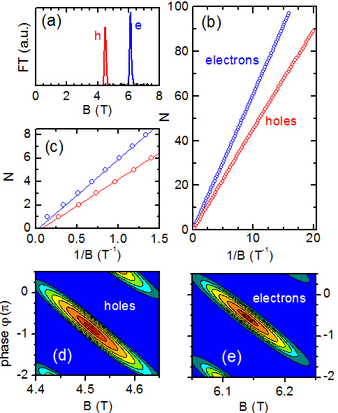
Figure 2: (color online) (a) Fourier transform of the low magnetic field $\Delta R_{xx}(1/B)$. (b-c) Orbital angular momentum quantum number N, as a function of the reciprocal magnetic field positions of the electron and hole features. (d) and (e) Contour plot of the phase shift function $K(\varphi,B)$ in the vicinity of the hole and electron features. Maxima in $K(\varphi,B)$ determines the frequency and phase of the oscillations.

In graphite, we have experimentally $\rho_{xx}\gg\rho_{xy}$ so that the tensor relation for conductivity simplifies to give $\sigma_{xx}\propto\rho_{xx}^{-1}$. Therefore, conductivity maxima which occur at coincidence of Landau bands and the Fermi energy $E_{F}$ Adams and Holstein (1958), correspond to minima in $\Delta R_{xx}(B)$. We perform a classical 1/B analysis of our data assigning an orbital quantum number N to the electron and hole minima of $\Delta R_{xx}(B)$. For $N<25$ the magnetic field positions of each series of oscillations can be determined directly from $\Delta R_{xx}(B)$. For $N>25$, pass band frequency domain filtering was used to separate the superimposed electron and hole features. The position of the features in inverse magnetic field versus N is shown in Fig. 2(b). For both electrons and holes we can see features with angular quantum number $1<N<90$ (to almost $N=100$ for electrons). $N$ versus $1/B$ has a linear dependence and the slope gives the fundamental fields $B_{F_{e}}=6.10\pm 0.05$ T and $B_{F_{h}}=4.50\pm 0.05$ T, in good agreement with the values obtained from the Fourier transform.

At low magnetic fields, i.e. at high quantum number N, a perfect linear behavior in $N(1/B)$ is observed for both electrons and holes. For high magnetic fields, i.e. for low $N$, clear deviations from the linear behavior are observed for the electron features (see Fig. 2(c)). This deviation from a periodic in 1/B behavior at high magnetic fields is due to the Fermi level moving as the quantum limit is approached in graphite Sugihara and Ono (1966); Woollam (1971). Clearly, the high field data should not be used to extract the phase of the oscillations Luk’yanchuk and Kopelevich (2006). Equally, extrapolating the low field data to find the intercept does not give a reliable estimate of the phase. Instead, we prefer to use the phase shift analysis method developed by Luk’yanchuk and Kopelevich Luk’yanchuk and Kopelevich (2004), to extract the phase from the complex Fourier transform $\hat{f}(B)$ of the low magnetic field $\Delta R_{xx}(1/B)$. The phase shift function $K(\varphi,B)=Re[e^{-i\varphi}\hat{f}(B)]$ has maximum in the $\varphi-B$ plane which can be used to extract both the frequency ($B$) and phase ($\varphi$) of the oscillations. $K(\varphi,B)$ is plotted in Fig. 2(d-e) in the regions of the hole and electron features. From the maxima, the determined frequency and phase are $B_{f_{h}}=4.51$ T, $\varphi_{h}=-(0.56\pm 0.1)\pi$ and $B_{f_{e}}=6.14$ T, $\varphi_{e}=-(0.86\pm 0.1)\pi$ for the hole and electron features respectively. For HOPG a similar analysis gives $\varphi_{h}=-(1.04\pm 0.1)\pi$ and $\varphi_{e}=-(0.92\pm 0.1)\pi$.

The oscillatory conductivity can be written $\Delta\sigma\propto\cos(2\pi B_{f}/B-2\pi\gamma+\delta)$ with $\gamma=1/2$ for massive fermions and $\gamma=0$ for massless Dirac fermions Adams and Holstein (1958); Mikitik and Yu. V. Sharlai (2006). At low magnetic fields inter Landau level scattering is expected to dominate so that $\delta=\pi/4$ for a 3D corrugated Fermi surface ($\delta=0$ for a 2D cylindrical Fermi surface). The expected value of the phase $\varphi=-2\pi\gamma+\delta$ for massive 3D fermions ($\gamma=1/2$) is therefore $\varphi=-0.75\pi$ in reasonable agreement with the experimental phase for both electrons and holes. For HOPG the phase is also consistent with $\gamma=1/2$ but with $\delta\approx 0$. The value of $\gamma=1/2$ is in agreement with published results Soule et al. (1964); Williamson et al. (1965) and theoretical considerations Mikitik and Yu. V. Sharlai (2006). In contrast, the prediction for 2D massless Dirac fermions ($\gamma=0$) with $\varphi=0$ is completely inconsistent with the determined phase for both electrons and holes. We therefore conclude that there is no evidence from transport measurements for the existence of masseless Dirac fermions with a Berry phase $\gamma=0$. Nevertheless, there is compelling evidence from far-infrared absorption, for the existence of Dirac fermions at the $H$ point in graphite M. Orlita et al. (2008). Far infrared measurements probe carriers in the very close vicinity of the $H$ point where there is a maximum in the joint (initial and final) density of states. Transport measurements however, are sensitive to the density of states at $E_{F}$, which is modulated with increasing magnetic field, as the Landau bands cross the Fermi energy. For holes, maxima in the density of states correspond to Landau bands crossing $E_{F}$ for $k_{z}<0.5$, away from the $H$ point, where the dispersion is no longer linear and a priori there is no reason to expect the carriers to behave as Dirac fermions.

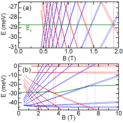
Figure 3: (color online) (a) Electron (increasing with B) and hole (decreasing with B) Landau bands ($dE/dk_{z}=0$) as a function of the magnetic field (calculated from SWM model for $B\geq 0.4$ T). The crossing of the electron and hole bands with the Fermi energy is in nearly perfect agreement with the measured magnetic field position of the electron (dotted lines) and hole (dashed lines) features. b) For $B\geq 2$ T, the Fermi energy is calculated self consistently, keeping the sum of the electron and hole concentrations constant.

It is interesting to compare the data with the predictions of the SWM 3D band structure model with its seven tight binding parameters $\gamma_{0},...,\gamma_{6}$. When the parameter $\gamma_{3}$ is taken into account the magnetic field Hamiltonian has infinite order. This was numerically reduced to a $600\times 600$ matrix for the exact diagonalization procedure. A maximum in the conductivity is expected when there is a maximum in the density of states at the Fermi level. This can be found, for a given magnetic field, by looking for a Landau band with a slope $dE/dk_{z}=0$ at $E_{F}$, which we refer to as a Landau band ‘crossing’ the Fermi level. Using the tight binding parameters of Ref. Brandt et al. (1988) as a starting point, this procedure was repeated until a satisfactory agreement with the data was obtained. The tight binding parameters found are given in Table 1. While we are unable to fit our data with exactly the same tight binding parameters as in Ref. Brandt et al. (1988), the values we find are nevertheless not significantly different. Moreover, the predicted Koshino and Ando (2007) effective mass, $m^{*}=4\hbar^{2}\gamma_{1}/3a_{0}^{2}\gamma_{0}^{2}=0.054m_{e}$ where $a_{0}=0.246$ nm is the in-plane lattice constant, calculated using our values for $\gamma_{0}$ and $\gamma_{1}$, is in good agreement with the accepted value Nozieres (1958).

	This work	Ref. Brandt et al. (1988)
$\gamma_{0}$ (eV)	$3.37\pm 0.02$	$3.16\pm 0.05$
$\gamma_{1}$ (eV)	$0.363\pm 0.05$	$0.39\pm 0.01$
$\gamma_{2}$ (eV)	$-0.0243\pm 0.001$	$-0.02\pm 0.002$
$\gamma_{3}$ (eV)	$0.31\pm 0.05$	$0.315\pm 0.015$
$\gamma_{4}$ (eV)	$0.07\pm 0.01$	$0.044\pm 0.024$
$\gamma_{5}$ (eV)	$0.05\pm 0.01$	$0.038\pm 0.005$
$\gamma_{6}=\Delta$ (eV)	$-0.007$	$-0.008\pm 0.002$
$E_{F}$ (eV)	$-0.0287$	$-0.024\pm 0.002$
$g_{s}$	$2.4\pm 0.1$	-
$n_{0}(\mathrm{cm}^{-3})$	$-(2.4\pm 0.4)\times 10^{17}$	-

Table 1: Summary of the SWM tight binding parameters found in this work and compared to the values given in Ref. Brandt et al. (1988).

For magnetic fields below $2$ T it is a good approximation to assume that the Fermi level is constant. The electron and hole Landau bands (solid lines), calculated using the parameters in Table 1, are plotted in Fig. 3(a) for magnetic fields below $2$ T. The vertical broken lines indicate the observed electron (dotted) and hole (dashed) minima in $\Delta R_{xx}$ (maxima in $\sigma_{xx}$). The agreement between the magnetic field position of the Landau bands crossing the Fermi level and the features in the transport data is remarkable.

At higher magnetic fields, as graphite approaches the quantum limit, the Fermi energy is no longer constant as carriers are transferred between the electron and hole pockets. This is the reason for the considerable deviation from 1/B periodicity observed at high magnetic fields in Fig. 2(c). Nevertheless, as can be seen in Fig. 3(b), the SWM model can correctly predict the magnetic field position of the features provided the movement of $E_{F}$ is taken into account. Here the Fermi level has been calculated self-consistently assuming the sum of the electron and hole concentrations is constant, $n-p=n_{0}$. The electron concentration corresponds to the number of states in partially filled bands below the Fermi energy, and the hole concentration to those above the Fermi energy. In order to fit the low–field data, we have used $n_{0}=-2.4\times 10^{17}$ $\mathrm{cm}^{-3}$, assuming that under neutrality conditions, $n=p=8\times 10^{18}$ $\mathrm{cm}^{-3}$, with $n=64\gamma_{1}|\gamma_{2}|/(9\sqrt{3}\pi^{2}\gamma_{0}^{2}a_{0}^{2}c_{0})$ Brandt et al. (1988).

To reproduce the spin splitting in the high magnetic field data, a g-factor $g_{s}=2.4$ is required. In graphite, the g-factor cannot be reliably estimated from the separation $\Delta B$ of the spin split features since the Fermi energy is moving with field Woollam (1970). While this does not noticeably shift the orbital features below $B=2$ T, the shift is significant compared to the spin gap. The value $g_{s}=2.4$ should be considered as a lower limit. Any significant Landau level broadening, neglected in our model, would reduce the movement of the Fermi energy, and therefore increase the value of $g_{s}$ required to fit the data.

To conclude, low temperature magnetotransport data of natural graphite and HOPG can be fully explained using the Slonczewski–Weiss–McClure tight binding model for massive fermions. No evidence for Dirac fermions at the $H$ point is observed in the transport data. This can be understood, since transport is dominated by the crossing of the Landau bands at the Fermi level, corresponding to $dE/dk_{z}=0$, which occurs away from the $H$ point ($k_{z}=0.5$), where the carriers are indeed Dirac fermions A. Grüneis et al. (2008); M. Orlita et al. (2008).