Local Linear Analysis of Interaction between a Planet and Viscous Disk and an Implication on Type I Planetary Migration

Abstract

We investigate the effects of viscosity on disk-planet interaction and discuss how type I migration of planets is modified. We have performed a linear calculation using shearing-sheet approximation and obtained the detailed, high resolution density structure around the planet embedded in a viscous disk with a wide range of viscous coefficients. We use a time-dependent formalism that is useful in investigating the effects of various physical processes on disk-planet interaction. We find that the density structure in the vicinity of the planet is modified and the main contribution to the torque comes from this region, in contrast to inviscid case. Although it is not possible to derive total torque acting on the planet within the shearing-sheet approximation, the one-sided torque can be very different from the inviscid case, depending on the Reynolds number. This effect has been neglected so far but our results indicate that the interaction between a viscous disk and a planet can be qualitatively different from an inviscid case and the details of the density structure in the vicinity of the planet is critically important.

1 Introduction

Disk-planet interaction and type I planetary migration is one of the main issues in the theory of planet formation. A low mass planet or the core of the gas giant planet embedded in the protoplanetary disk excites spiral density wave in the disk, which carries angular momentum flux away from the planet. The linear calculation of the spiral density wave is first carried out by Goldreich and Tremaine (1979), and there has been a number of extensive work assuming inviscid, isothermal disk such as Ward (1986, 1989), Artymowicz (1993), and Tanaka et al. (2002). In the case of an inviscid, isothermal disk, protoplanets migrate towards the central star as a result of disk-planet interaction very rapidly, thereby imposing a serious problem on the theory of planet formation.

The decay of the orbital semi-major axis of the protoplanet is a result of the subtle difference between the inner disk (the part of the disk inside the orbit of the protoplanet) and the outer disk (the part of the disk outside the orbit of the protoplanet). The outer disk exerts torque on the protoplanet in such a way that the semi-major axis decreases, and the inner disk exerts opposite torque. In the lowest order of the local approximation, or shearing-sheet approximation, these two effects cancel each other, and the difference appears at higher order. Therefore, type I migration can be very sensitive to the physical state of the disk. Indeed, when non-isothermal effect is taken into account, the direction of migration can be reversed (Paardekooper and Mellema 2006, Baruteau and Masset 2008, Paardekooper and Papaloizou 2008). It is also discussed that the global magnetic field can slow down the rate of type I migration or even reverse the direction (Terquem 2003, Fromang et al. 2005, Muto et al. 2008).

In order to construct a predictable, self-consistent model for planet formation, it is important to make clear how different physical processes of the disk affect disk-planet interaction and type I migration. In this paper, we revisit the effects of viscosity on disk-planet interaction. There has been a number of work on this topic. Meyer-Vernet and Sicardy (1987) discussed that the viscosity does not affect the torque exerted on the planet as long as its value is small, although the shape of the wake may be modified. Papaloizou and Lin (1984, and a series of their paper) and Takeuchi et al. (1996) calculated that the damping of the density wave and the transfer of the angular momentum from the density wave to the background disk, resulting in the gap formation around a massive planet. Masset (2001) investigated the effects of viscosity on the horseshoe regions and discussed how the corotation torque may be altered by the effect of viscosity. More recently, Paardekooper and Papaloizou (2009b) investigated the dynamics of corotation region using both linear and non-linear calculations.

Although there has been a number of investigations on the disk-planet interaction in a viscous disk (for example, Masset 2001, 2002 or Paardekooper and Papaloizou 2009a for corotation torque, D’Angelo et al. 2002, 2003 for high resolution numerical study), there has not yet been a study of wide range in the viscous coefficient that requires an analysis on the detailed density structure in the vicinity of the planet. In this paper, as a first step for the complete investigation, we show results of linear calculation in a local, shearing-sheet analysis. We use time-dependent methods to calculate the disk response against the planet potential. Although this method has not been widely used so far, this is useful in investigating the effects of various physical processes on disk-planet interaction. We calculate the non-axisymmetric density structure around the planet and investigate how the resulting torque is altered by the effect of shear viscosity. We have studied wide range of the parameters of viscous coefficient and calculate the density structure with high resolution. We find that the density structure in the vicinity of the planet is altered in a viscous disk, with viscous coefficient of $\sim 0.1$ in terms of $\alpha$ (standard $\alpha$ parameter, see equation (27) for definition), which may be realized as a result of the turbulence induced by magneto-rotational instability (MRI, Balbus and Hawley 1991, Sano et al. 2004).

Since it is not possible to calculate the total torque (differential torque between the disk inside the orbit of the planet and outside) in shearing-sheet approximation, we look at one-sided torque to investigate how type I migration rate can be affected qualitatively by viscosity. One-sided torque is the torque exerted by one side of the disk with respect to the planet’s orbital radius. We also note that shearing-sheet calculation is a useful first step before differential torque is calculated (Tanaka et al. 2002). We find that as we increase the values of viscous coefficient $\alpha$, one-sided torque stays unchanged until $\alpha\mathrel{\hbox{\hbox to0.0pt{\hbox{\lower 4.0pt\hbox{$\sim$}}\hss}\hbox{$<$}}}0.01$, then increases until $\alpha\sim 1$, and finally decreases. The torque can be factor of two larger than inviscid case when $\alpha=0.1$, and more importantly, the enhancement of the torque is a result of the modified density structure in the vicinity of the planet, which has not yet been investigated in detail. Our results indicate that the physical mechanisms of the disk-planet interaction in a viscous disk may depend on the detailed density structure around the planet.

The plan of this paper is as follows. In section 2 we show the basic equations and describe the time-dependent methods to obtain a stationary, non-axisymmetric pattern of linear perturbation. We also discuss how two-dimensional (2D) and three-dimensional (3D) analyses are related in this section. In section 3, we show the results of 2D and 3D calculations and show how the torque behaves as we vary the amount of viscosity. In section 4, we explain the qualitative behavior of the torque using a simple analytic model. Section 5 is for discussion and summary.

2 Basic Equations and Numerical Methods

2.1 Linear Perturbation Analysis

We consider isothermal Navier-Stokes equations with one planet using shearing-sheet approximation.

$${\displaystyle\frac{\partial\rho}{\partial t}}+\nabla\cdot(\rho\mbox{\boldmath$v$})=0$$ (1)

$${\displaystyle\frac{\partial\mbox{\boldmath$v$}}{\partial t}}+\mbox{\boldmath$v$}\cdot\nabla\mbox{\boldmath$v$}+2\Omega_{\rm p}\mbox{\boldmath$e$}_{z}\times\mbox{\boldmath$v$}=-{\displaystyle\frac{c^{2}}{\rho}}\nabla{\rho}+3\Omega^{2}_{\rm p}x\mbox{\boldmath$e$}_{x}+\nu\nabla^{2}\mbox{\boldmath$v$}+{\displaystyle\frac{1}{3}}\nu\nabla(\nabla\cdot\mbox{\boldmath$v$})-\nabla\psi_{\rm p}$$ (2)

where $\rho$ is density, $v$ is velocity, $\Omega_{\rm p}$ is the Kepler angular velocity of the planet, $\psi_{\rm p}$ is the gravitational potential of the planet, $\nu$ is shear viscosity. The third term of left hand side of equation (2) is Coriolis force and the second term of right hand side of equation (2) is tidal force. We assume the planet is located at the origin and stationary with respect to this coordinate system, i.e.,

$$\psi_{\rm p}=\psi_{\rm p}(x,y,z),$$ (3)

where $\psi_{\rm p}$ does not depend on time. In this paper, we neglect bulk viscosity for simplicity. We also neglect vertical stratification and assume that the background density without a planet is homogeneous. This gives an uncertainty in the box size in the $z$-direction, which will be discussed in Section 2.2. We also neglect the effect of global gas pressure gradient exerted on the background disk and assume that the background gas is rotating at Kepler velocity.

The unperturbed state without a planet is given by

$$\rho=\rho_{0}=\mathrm{const}$$ (4)

$$\mbox{\boldmath$v$}_{0}=-{\displaystyle\frac{3}{2}}\Omega_{\rm p}x\mbox{\boldmath$e$}_{y}.$$ (5)

In the presence of viscosity, if we perform a global analysis, there is a mass accretion onto the central star in general. However, in the shearing-sheet approximation, where linear background shear is assumed, this effect is not taken into account. We expect that the density structure only in the vicinity of the planet can be well approximated even if we neglect the global mass accretion.

We consider linear perturbation. All the perturbation quantities are denoted with $\delta$, e.g., $\delta\rho$ for density perturbation. Perturbation equations are given by

$$\left({\displaystyle\frac{\partial}{\partial t}}-{\displaystyle\frac{3}{2}}\Omega_{\rm p}x{\displaystyle\frac{\partial}{\partial y}}\right){\displaystyle\frac{\delta\rho}{\rho_{0}}}+\nabla\cdot\delta\mbox{\boldmath$v$}=0$$ (6)

$$\left({\displaystyle\frac{\partial}{\partial t}}-{\displaystyle\frac{3}{2}}\Omega_{\rm p}x{\displaystyle\frac{\partial}{\partial y}}\right)\delta\mbox{\boldmath$v$}-2\Omega_{\rm p}\delta v_{y}\mbox{\boldmath$e$}_{x}+{\displaystyle\frac{1}{2}}\Omega_{\rm p}\delta v_{x}\mbox{\boldmath$e$}_{y}$$

$$=-c^{2}\nabla{\displaystyle\frac{\delta\rho}{\rho_{0}}}+\nu\nabla^{2}\delta\mbox{\boldmath$v$}+{\displaystyle\frac{1}{3}}\nu\nabla\left(\nabla\cdot\delta\mbox{\boldmath$v$}\right)-\nabla\psi_{\rm p}$$ (7)

We solve equations (6) and (7) to obtain a steady state solution and calculate torque exerted on one side (either $x>0$ or $x<0$) of the disk by the planet. The torque exerted on the planet is obtained as a backreaction of this torque. Since we use shearing-sheet approximation, torque exerted from each side of the planet is the same in magnitude and opposite in sign. Although we do not obtain a net torque, it is still possible to investigate how the disk structure is affected by the viscosity and qualitatively predict how the disk and planet interact.

In order to obtain a steady state solution, we solve linear perturbation equations (6) and (7) using Fourier transform methods given by Goodman and Rafikov (2001). We transform the equations into the shearing coordinate $(t^{\prime},x^{\prime},y^{\prime},z^{\prime})$ defined by

$$t^{\prime}=t$$ (8)

$$x^{\prime}=x$$ (9)

$$y^{\prime}=y+{\displaystyle\frac{3}{2}}\Omega_{\rm p}xt$$ (10)

$$z^{\prime}=z.$$ (11)

In this coordinate system, temporal and spatial derivatives are given by

$${\displaystyle\frac{\partial}{\partial t}}={\displaystyle\frac{\partial}{\partial t^{\prime}}}+{\displaystyle\frac{3}{2}}\Omega_{\rm p}x^{\prime}{\displaystyle\frac{\partial}{\partial y^{\prime}}},$$ (12)

$${\displaystyle\frac{\partial}{\partial x}}={\displaystyle\frac{\partial}{\partial x^{\prime}}}+{\displaystyle\frac{3}{2}}\Omega_{\rm p}t^{\prime}{\displaystyle\frac{\partial}{\partial y^{\prime}}},$$ (13)

$${\displaystyle\frac{\partial}{\partial y}}={\displaystyle\frac{\partial}{\partial y^{\prime}}},\ {\displaystyle\frac{\partial}{\partial z}}={\displaystyle\frac{\partial}{\partial z^{\prime}}}.$$ (14)

Then, perturbation equations become

$${\displaystyle\frac{\partial}{\partial t^{\prime}}}{\displaystyle\frac{\delta\rho}{\rho_{0}}}+\nabla\cdot\delta\mbox{\boldmath$v$}=0$$ (15)

$${\displaystyle\frac{\partial}{\partial t^{\prime}}}\delta\mbox{\boldmath$v$}-2\Omega_{\rm p}\delta v_{y}\mbox{\boldmath$e$}_{x}+{\displaystyle\frac{1}{2}}\Omega_{\rm p}\delta v_{x}\mbox{\boldmath$e$}_{y}$$

$$=-c^{2}\nabla{\displaystyle\frac{\delta\rho}{\rho_{0}}}+\nu\nabla^{2}\delta\mbox{\boldmath$v$}+{\displaystyle\frac{1}{3}}\nu\nabla\left(\nabla\cdot\delta\mbox{\boldmath$v$}\right)-\nabla\psi_{\rm p},$$ (16)

where the spatial derivatives in $\nabla$ are given by equations (13) and (14).

The coefficients of equation (15) and (16) are now independent of $(x^{\prime},y^{\prime},z^{\prime})$. Therefore, if we Fourier transform in spatial directions, we obtain a set of ordinary differential equations decoupled for each $(k_{x}^{\prime},k_{y}^{\prime},k_{z}^{\prime})$ mode (Goldreich and Lynden-Bell 1965),

$$\delta f(t^{\prime},x^{\prime},y^{\prime},z^{\prime})=\sum\delta f(t^{\prime},k_{x}^{\prime},k_{y}^{\prime},k_{z}^{\prime})\exp\left[i(k_{x}^{\prime}x^{\prime}+k_{y}^{\prime}y^{\prime}+k_{z}^{\prime}z^{\prime})\right].$$ (17)

The relationship of wavenumber in $(x,y,z)$-coordinate and $(x^{\prime},y^{\prime},z^{\prime})$-coordinate is given by

$$k_{x}(t)=k_{x}^{\prime}+{\displaystyle\frac{3}{2}}\Omega_{\rm p}k_{y}t.$$ (18)

$$k_{y}=k_{y}^{\prime},\ k_{z}=k_{z}^{\prime}$$ (19)

Equation (18) indicates that the value of radial wavenumber in $(x,y,z)$-coordinate evolves with time owing to the background shear. The value of radial wavenumber in shearing coordinate $k_{x}^{\prime}$ gives the initial value of radial wavenumber in $(x,y,z)$-plane. Equations of continuity (6) and motion (7) are now

$${\displaystyle\frac{d}{dt}}{\displaystyle\frac{\delta\rho}{\rho_{0}}}+ik_{x}(t)\delta v_{x}+ik_{y}\delta v_{y}+ik_{z}\delta v_{z}=0,$$ (20)

$${\displaystyle\frac{d}{dt}}\delta v_{x}-2\Omega_{\rm p}\delta v_{y}=-c^{2}ik_{x}(t){\displaystyle\frac{\delta\rho}{\rho_{0}}}-\nu(k_{x}(t)^{2}+k_{y}^{2}+k_{z}^{2})\delta v_{x}$$

$$-{\displaystyle\frac{1}{3}}\nu k_{x}(t)(k_{x}(t)\delta v_{x}+k_{y}\delta v_{y}+k_{z}\delta v_{z})-ik_{x}(t)\psi_{\rm p},$$ (21)

$${\displaystyle\frac{d}{dt}}\delta v_{y}+{\displaystyle\frac{1}{2}}\Omega_{\rm p}\delta v_{x}=-c^{2}ik_{y}{\displaystyle\frac{\delta\rho}{\rho_{0}}}-\nu(k_{x}(t)^{2}+k_{y}^{2}+k_{z}^{2})\delta v_{y}$$

$$-{\displaystyle\frac{1}{3}}\nu k_{y}(k_{x}(t)\delta v_{x}+k_{y}\delta v_{y}+k_{z}\delta v_{z})-ik_{y}\psi_{\rm p},$$ (22)

and

$${\displaystyle\frac{d}{dt}}\delta v_{z}=-c^{2}ik_{z}{\displaystyle\frac{\delta\rho}{\rho_{0}}}-\nu(k_{x}(t)^{2}+k_{y}^{2}+k_{z}^{2})\delta v_{y}$$

$$-{\displaystyle\frac{1}{3}}\nu k_{y}(k_{x}(t)\delta v_{x}+k_{y}\delta v_{y}+k_{z}\delta v_{z})-ik_{z}\psi_{\rm p}.$$ (23)

In equations (20)-(23), we write all the terms in $(t,x,y,z)$-coordinate. These equations describe the excitation and evolution of density wave by the source $\psi_{\rm p}$. The source of the density wave becomes zero when wavenumber $(k_{x}^{\prime},k_{y}^{\prime},k_{z}^{\prime})$ is large.

As an initial condition, we assume that there is no perturbation: $\delta\rho(t=0)=\delta\mbox{\boldmath$v$}(t=0)=0$, and $k_{x}^{\prime}$ is taken to be sufficiently large in absolute magnitude and negative (positive) in sign for positive (negative) $k_{y}$. If we use spatial resolution of $x$-direction $\Delta x$, we should take $k_{x}^{\prime}=\mp 2\pi/\Delta x$, where upper (lower) sign is used for positive (negative) $k_{y}$. As a result of time evolution, $k_{x}(t)$ increases (decreases) for each positive (negative) $k_{y}$ mode. When $k_{x}(t)$ reaches $\pm 2\pi/\Delta x$, where upper (lower) sign is for positive (negative) $k_{y}$ modes, we obtain a steady state profile of perturbation quantities in Fourier space for non-axisymmetric ($k_{y}\neq 0$) modes. The Fourier amplitude of each $k_{x}$ mode in steady state is given by the time evolution data through equation (18). The profile of physical quantities in Fourier space is then inverse Fourier transformed to obtain values in real space. Since we are interested in torque, we do not calculate axisymmetric modes ($k_{y}=0$).

The standard procedure to obtain steady state solution is as follows. Firstly, stationary solution in the frame corotating with the planet is assumed: $\partial/\partial t=0$. Then, Fourier transformation in the $y$- and $z$-directions is performed to obtain the ordinary differential equations in the $x$-direction. Finally, these ordinary differential equations are solved by imposing outgoing boundary condition, or equivalently the boundary condition that admits only trailing wave, see e.g., Goldreich and Tremaine (1979), Korycansky and Pollack (1993), or Tanaka et al. (2002).

In the presence of viscosity, this method introduces higher order derivative with respect to $x$, since viscous terms include the second order derivative in the radial direction. The resulting ordinary differential equations are higher order in the $x$-derivative than in inviscid cases. The terms with the highest order derivative comes from viscous terms and their coefficients are viscous coefficient $\nu$. In this case, it is difficult to take natural $\nu\to 0$ limit, since equations become singular in this limit.

Time-dependent approach overcomes this difficulty since the order of time derivative is not affected by viscous terms since they do not include any time derivative. It is also easy to take $\nu\to 0$ limit since viscous terms simply drop from equations (21)-(23) in this limit and they do not introduce any singularity.

In our formulation using the Fourier transform in sheared coordinate, the outgoing boundary condition in the radial direction that is assumed in the standard stationary formulation is not exactly satisfied, since Fourier transform introduces the periodic boundary condition in the sheared coordinate. However, we find that outgoing boundary condition is effectively satisfied if we vary the box size in the $x$-direction depending on the modes specified by $k_{y}$ and $k_{z}$. Details of our methods are given below.

We also note that if we assume an initial condition with non-zero perturbation, additional homogeneous wave is introduced. This wave has both leading ($k_{x}k_{y}<0$) and trailing ($k_{x}k_{y}>0$) components and the resulting solution is simply the superposition of the specific solution of Equations (20)-(23) assuming zero initial condition and homogeneous ($\psi_{\rm p}=0$) solution assuming the specified initial condition. The solution with non-zero initial condition is irrelevant in the present problem because we consider the perturbation that is induced by the gravitational perturbation by the planet.

We write the box size in $(x,y,z)$-directions by $(L_{x},L_{y},L_{z})$ and the coordinate system extends $-L_{x}/2<x<L_{x}/2$ and so forth for other directions. Practically, our procedure to obtain the stationary, non-axisymmetric structure of the disk is summarized as follows.

1. We take $k_{x}^{\prime}=\mp 2\pi/\Delta x$ for positive (negative) $k_{y}$ modes.

2. Equations (20)-(23) are solved with initial condition $\delta\rho(t=0)=\delta\mbox{\boldmath$v$}(t=0)=0$.

3. Resulting solutions in $(k_{x},k_{y},k_{z})$ space are inverse Fourier transformed to real space.

In steps 2 and 3, there are some points we need to take care. In calculating the Fourier modes, we have varied the mesh number in $k_{x}$ directions, which corresponds to the step size of time, in such a way that all the oscillations are well resolved for each $(k_{y},k_{z})$ mode. The mesh number in $k_{x}$ direction becomes as much as $10^{6}$ for small $k_{y}$. We perform inverse Fourier transform in $k_{x}$ direction using the increased number of mesh in $k_{x}$ direction. This procedure effectively makes the box size of $x$-direction longer for a specific $k_{y}$ mode, and the data corresponding to necessary $x$, which is $-L_{x}/2<x<L_{x}/2$, is then interpolated from the resulting profile in $(x,k_{y},k_{z})$ space. This data is then used to perform inverse Fourier transform in $(k_{y},k_{z})$ directions. In this way, it is possible to avoid aliasing effect in $x$-direction and outgoing boundary condition in the steady state solution is effectively satisfied. We do not use any window function, which has been incorporated by Goodman and Rafikov (2001), in Fourier transform. We have checked that the resulting torque is not affected by the window function in the absence of viscosity. Also, since window function introduces additional artificial dissipation, this affects our results with viscosity.

Once we have obtained the profiles of perturbation quantities in real space, we can calculate the one-sided torque exerted on $x>0$ part of the disk by the planet by

$$T=-r_{\rm p}\int_{0}^{L_{x}}\int_{-L_{y}/2}^{L_{y}/2}\int_{-L_{z}/2}^{L_{z}/2}dxdydz\delta\rho(x,y,z){\displaystyle\frac{\partial\psi_{\rm p}}{\partial y}},$$ (24)

where $r_{p}$ is the semi-major axis of the planet, and the torque exerted on the planet is obtained as backreaction. For later convenience, we define “torque distribution” $T(x,y,z)$ that is simply the torque exerted on the fluid element located at $(x,y,z)$,

$$T(x,y,z)=-r_{\rm p}\delta\rho(x,y,z){\displaystyle\frac{\partial\psi_{\rm p}}{\partial y}}$$ (25)

and “torque density” that is the torque exerted on an annulus of the disk at $x$,

$$T(x)=-r_{\rm p}\int_{-L_{y}/2}^{L_{y}/2}\int_{-L_{z}/2}^{L_{z}/2}dzdy\delta\rho(x,y,z){\displaystyle\frac{\partial\psi_{\rm p}}{\partial y}}$$ (26)

We normalize equations using $c$, $\Omega_{\rm p}$, and $\rho_{0}$ so that the homogeneous equations ($\psi_{\rm p}$=0) contain only one dimensionless variable $\alpha$ that is defined by

$$\alpha={\displaystyle\frac{\nu}{cH}},$$ (27)

where $H=c/\Omega_{\rm p}$ is the scale height of the disk. Since we consider the linear perturbation analysis, the amplitude of the perturbation is proportional to the normalized planet mass:

$$\mu=GM_{\rm p}/Hc^{2}.$$ (28)

We show the results with $\mu=1$ in subsequent sections.

We use the fifth order Runge-Kutta method to solve time evolution and FFT routine given by Press et al. (1992) to perform Fourier transform. We use box size of $L_{x}=10H$ and $L_{y}=40H$, and the grid number in $x$- and $y$-directions $(N_{x},N_{y})=(512,512)$. The three-dimensional results depend on the box size in $z$-direction, $L_{z}$, which is discussed in the next subsection.

2.2 Vertical Box Size and the Difference between 2D and 3D Calculation

In this subsection, we discuss how 2D and 3D calculations differ from each other and determine the relevant box size in the $z$-direction with which the effect of vertical stratification is effectively taken into account.

We compare 2D calculation and 2D mode of 3D calculation. By “2D calculation”, we mean the gravitational potential of the planet is given by

$$\psi_{\rm p,2D}(x,y)=-{\displaystyle\frac{GM_{\rm p}}{\sqrt{x^{2}+y^{2}+\epsilon_{\rm 2D}^{2}}}},$$ (29)

where $\epsilon_{\rm 2D}$ denotes the softening length of 2D calculation, which is usually incorporated in most of 2D work. By “2D mode of 3D calculation”, we mean that the analysis is restricted to $k_{z}=0$ mode of 3D calculation. Three-dimensional potential is given by

$$\psi_{\rm p,3D}(x,y,z)=-{\displaystyle\frac{GM_{\rm p}}{\sqrt{x^{2}+y^{2}+z^{2}+\epsilon_{\rm 3D}^{2}}}}.$$ (30)

Therefore, gravitational potential for “2D mode of 3D calculation” is given by

$$\psi_{\rm p,3D}(x,y) =-{\displaystyle\frac{1}{L_{z}}}\int_{-L_{z}/2}^{L_{z}/2}dz{\displaystyle\frac{GM_{\rm p}}{\sqrt{x^{2}+y^{2}+z^{2}+\epsilon_{\rm 3D}^{2}}}}$$ (31)

$$=-{\displaystyle\frac{GM_{\rm p}}{L_{z}}}\log\left|{\displaystyle\frac{x^{2}+y^{2}+\epsilon_{\rm 3D}^{2}+L_{z}^{2}/2+L_{z}\sqrt{L_{z}^{2}/4+x^{2}+y^{2}+\epsilon_{\rm 3D}^{2}}}{x^{2}+y^{2}+\epsilon_{\rm 3D}^{2}}}\right|,$$

where we denote softening length in 3D calculation by $\epsilon_{\rm 3D}$. We note that $\psi_{\rm p,2D}$ and $\psi_{\rm p,3D}$ coincides if $x^{2}+y^{2}+\epsilon^{2}\gg L_{z}$, but they differ if $x^{2}+y^{2}+\epsilon^{2}\ll L_{z}$, since in this case, 3D potential behaves as $\psi_{\rm p,3D}\sim\log r$ while 2D potential behaves as $\psi_{\rm p,2D}\sim 1/r$, where $r^{2}=x^{2}+y^{2}+\epsilon^{2}$. Vertical averaging makes the potential weaker in the vicinity of the planet, thereby producing small perturbation in 2D mode of 3D calculation. Figure 1 shows the torque obtained by 2D inviscid ($\nu=0$) calculation using $\psi_{\rm p,2D}$ and $\psi_{\rm p,3D}$ with various $L_{z}$. We note that in producing Figure 1, one-sided torque is calculated according to equation (24) and the value is normalized by

$$\Gamma_{\rm 2D}=\mu^{2}\rho_{0}L_{z}r_{\rm p}Hc^{2}.$$ (32)

It is clear that 2D and 3D results coincide if $L_{z}$ is small, but the 3D result becomes small when $L_{z}$ is large.

The reasonable value of $L_{z}$ may be obtained by comparing the results of 2D mode of 3D calculation with calculation in which vertical stratification is taken into account. Tanaka et al. (2002) performed such calculations for an inviscid disk. Their method is to decompose vertical modes in terms of Hermite polynomials, and they have found that the vertically averaged 2D mode gives most of the contribution to the resulting torque. Their 2D mode of the potential, $\psi_{\rm p,TTW}$, is given by

$$\psi_{\rm p,TTW} =-{\displaystyle\frac{1}{\sqrt{2\pi}H}}\int_{-\infty}^{\infty}dz{\displaystyle\frac{GM_{\rm p}}{\sqrt{x^{2}+y^{2}+z^{2}+\epsilon_{\rm 3D}^{2}}}}e^{-z^{2}/2H^{2}}$$ (33)

$$=-{\displaystyle\frac{GM_{\rm p}}{\sqrt{2\pi}H}}\exp\left[(x^{2}+y^{2}+\epsilon_{\rm 3D}^{2})/4\right]K_{0}\left[\left(x^{2}+y^{2}+\epsilon_{\rm 3D}^{2}\right)/4\right],$$

where $K_{0}(x)$ is the modified Bessel function of the zeroth order. Fitting equation (31) with equation (33), we find $L_{z}=2.7H$ gives a reasonable agreement, see Figure 2. Zeroth order of modified local approximation incorporated by Tanaka et al. (2002) coincides with the shearing-sheet approximation, and we have exactly the same homogeneous equations with them for 2D ($k_{z}=0$) mode if we assume $\partial/\partial t=0$. As is clear from Figure 1, 2D mode in 3D calculation gives smaller amount of torque than the calculation using 2D potential given by equation (29). This explains why Tanaka et al. (2002) has obtained slightly smaller amount of torque compared to 2D results. We have also checked that setting $L_{z}=2.7H$, our results of one-sided torque agree with those determined by using Tanaka et al. (2002) methods within an error of $3\%$.

We use $L_{z}=2.5H$ and the mesh number in $z$-direction is taken to be $128$. In total, we have performed calculation with $(L_{x},L_{y},L_{z})=(10H,40H,2.5H)$ with mesh number $(512,512,128)$, and the resulting mesh size is $(\Delta x,\Delta y,\Delta z)=(0.02H,0.08H,0.02H)$. However, the radial box size is variably extended according to modes in calculation, as discussed in Section 2.1. Effective box size in $x$-direction is as much as $10^{4}H$. We use $\epsilon_{\rm 3D}=10^{-3}H$ for the softening parameter. Our results vary upto $30\%$ for large values of viscosity when smoothing length is varied upto twice the grid resolution. Therefore, our results give at least a qualitative view of how disk-planet interaction is altered by the effects of viscosity. The variation of one-sided torque as a function of smoothing parameter is further discussed in Section 3.2.

3 Results

In this section, we show our results of density structure and one-sided torque obtained by linear analysis. In this section, the normalization of the torque is given by

$$\Gamma_{\rm 3D}=\mu^{2}\rho_{0}r_{\rm p}H^{2}c^{2}.$$ (34)

Note the difference in the normalization from that used in Section 2.2. The results of 2D mode torque given in Section 3.1 are different by a factor of $L_{z}/H=2.5$ from those given in Figure 1. The normalization of torque distribution defined by equation (25) is taken to be

$${\displaystyle\frac{T(x,y,z)}{\mu^{2}\rho_{0}r_{\rm p}c^{2}H^{-1}}},$$ (35)

and torque density $T(x)$ defined by equation (26) is given by

$${\displaystyle\frac{T(x)}{\mu^{2}\rho_{0}r_{\rm p}c^{2}}}.$$ (36)

3.1 Calculations Restricted to 2D Mode

We first show the results of calculations restricted to 2D modes ($k_{z}=0$). Although this is only an approximation, physics involved is made clear. Figure 3 shows the torque obtained for various viscosity parameter $\alpha$. For small viscous coefficients ($\alpha\mathrel{\hbox{\hbox to0.0pt{\hbox{\lower 4.0pt\hbox{$\sim$}}\hss}\hbox{$<$}}}10^{-2}$), torque is not affected by the viscosity, as discussed by Meyer-Vernet and Sicardy (1987). However, when viscous coefficient is large, it is shown that one-sided torque increases and peaks around $\alpha\sim 1$.

Since viscosity, or any form of dissipation, damps density contrast in general, one may think that Lindblad torque is a decreasing function of viscosity. However, our result shows that one-sided torque peaks at $\alpha\sim 1$. This result originates from two different effects of viscosity. First, viscosity damps spiral density wave, as discussed by Papaloizou and Lin (1984) or Takeuchi et al. (1996). The second effect of viscosity may be observed by looking at the density structure in the vicinity of the planet. Figure 4 shows the contour of density profile of the $xy$-plane for $\alpha=10^{-4}$ and $\alpha=10^{-1}$. It is clear that the oval density profile in the vicinity of the planet is slightly tilted for large viscous coefficient, while the spiral density wave is damped. This tilt produces asymmetry of density structure in the $y$-direction, thereby exerting one-sided torque on the planet.

Figure 5 shows the torque density for $\alpha=10^{-1}$ and $\alpha=10^{-4}$, respectively. It is clear that the peak of torque density locates slightly closer to the planet for $\alpha=10^{-1}$ than $\alpha=10^{-4}$. The main contribution to the torque comes from the flow structure in the vicinity of the planet, which is evident when we consider the asymmetry of the density perturbation between $y>0$ and $y<0$ regions. In Figure 6, we plot the contour for the sum of torque at $y>0$ and $y<0$ region,

$$T(x,y)+T(x,-y),$$ (37)

as a function of $x$ and $y(>0)$. This shows the asymmetry of torque distribution in the $y$-directions. In Figure 6, we compare the results for two different values of viscosity, $\alpha=10^{-4}$ and $\alpha=10^{-1}$. In the case of $\alpha=10^{-4}$, the forward-back difference of the torque in the vicinity of the planet almost vanishes since the density perturbation around the planet is symmetric in the $y$-direction. In the case of $\alpha=10^{-1}$, however, the most of the contribution to the torque comes from the region very close to the planet since the oval density perturbation structure is tilted in $y<0$ direction (see also Figure 4).

3.2 3D Calculation and the Effects of Smoothing Length

In this section, we present the results of 3D calculation. Figure 7 shows the one-sided torque as a function of viscosity. The qualitative behavior of torque increasing with viscosity is unchanged, but the enhancement of torque becomes large compared to 2D calculation. We fit the data and obtain the following empirical relation

$${\displaystyle\frac{T}{\rho_{0}r_{\rm p}H^{2}c^{2}}}=(0.94+10\alpha)e^{-1.5\alpha}$$ (38)

for $\alpha<0.3$ and $L_{z}=2.5H$. We have chosen a form of fitting function in such a way that torque converges to a non-zero value for $\alpha\ll 1$, peaks at $\alpha\sim 1$, and decreases to zero for $\alpha\gg 1$. This fitting formula is in reasonably good agreement with our calculation in this range of viscosity coefficient.

Just as in the calculations restricted to 2D modes, the density structure mainly in the vicinity of the planet contributes to the one-sided torque if large values of viscosity is assumed. Figure 8 shows the torque density profile obtained for different viscosity coefficients. The more viscous is the disk, the closer to the planet is the location of the dominant contribution to the torque. Figure 9 compares the density structure in the $yz$-plane at $x=0.068H$ for calculations with $\alpha=10^{-4}$ and $\alpha=10^{-1}$. The asymmetry in the $y$-direction in strongly perturbed region is present in calculations with large viscosity.

In 3D calculations, gravitational potential in the vicinity of the planet is not as strongly softened as in 2D modes. In the vicinity of the planet, gas feels the gravitational potential that decreases as $-1/r$, where $r$ is the distance from the planet, in full 3D calculations. However, the gravitational potential varies only logarithmically when $r\mathrel{\hbox{\hbox to0.0pt{\hbox{\lower 4.0pt\hbox{$\sim$}}\hss}\hbox{$<$}}}H$ (see equation (31)) in calculations restricted to 2D modes. Since the density fluctuation around the planet is given by $\delta\rho/\rho_{0}\sim\psi_{\rm p}/c^{2}$, the deeper gravitational potential gives the higher value of the torque exerted on the planet if there is a substantial asymmetry in the density structure.

Calculations restricted to two-dimensional modes predict one-sided torque very well if viscosity parameter is small, since regions close to the planet ($r\mathrel{\hbox{\hbox to0.0pt{\hbox{\lower 4.0pt\hbox{$\sim$}}\hss}\hbox{$<$}}}H$) is not very important. However, if large values of viscosity is used, it is necessary to perform full three-dimensional calculations since the density structure close to the planet is important.

At the end of Section 2.2, we addressed that varying smoothing length changes one-sided torque upto $30\%$. Below, we discuss the effects of smoothing length in our calculation and argue that the values of one-sided torque obtained for large viscosity, $\alpha\mathrel{\hbox{\hbox to0.0pt{\hbox{\lower 4.0pt\hbox{$\sim$}}\hss}\hbox{$>$}}}0.01$, seems to be the lower limit of the one-sided torque.

Figure 10 shows how one-sided torque of three-dimensional calculation varies with smoothing length $\epsilon_{\rm 3D}$. Results with $\alpha=10^{-4}$ and $\alpha=10^{-1}$ are shown. In this calculation, we used the box size with $(L_{x},L_{y},L_{z})=(10H,10H,2.5H)$ and the grid number with $(N_{x},N_{y},N_{z})=(512,512,128)$. Note that resolution in the $y$-direction is better by a factor of four compared to the parameters used in Figure 7. Grid resolution is $\sim 0.02H$ in all directions in Figure 10.

It is shown that one-sided torque converges well for small values of viscosity parameter. If $\alpha$ is as large as $0.1$, the calculation converges for sub-grid smoothing lengths, and results vary approximately $30\%$ if smoothing length with twice the grid scale ($\sim 0.04H$) is assumed. The qualitative behavior of one-sided torque can be understood if we notice that smaller smoothing length gives a deeper potential in the vicinity of the planet, and if large values of viscosity is assumed, density structure in the vicinity of the planet is important for one-sided torque.

Since contribution to one-sided torque in case of large viscosity mainly comes from the density structure close to the planet, it may depend on the grid resolution used in the calculation. Figure 11 shows the one-sided torque obtained for different resolutions. Calculations with $(N_{x},N_{y},N_{z})=(512,512,128)$, $(256,256,64)$, and $(128,128,32)$ are shown while keeping $(L_{x},L_{y},L_{z})=(10H,10H,2.5H)$. These values corresponds to grid resolutions with $\Delta x=\Delta y=\Delta z=0.02H$, $0.04H$, and $0.08H$, respectively. The value of softening parameter is kept $\epsilon_{\rm 3D}=10^{-3}H$ for all the calculations. It is shown that the value of one-sided torque for $\alpha=10^{-4}$ is well converged while the value of the torque for $\alpha=10^{-1}$ varies approximately $30\%$ when grid resolution is varied by a factor of four. We note that in case of small viscosity, we have obtained well-converged values of one-sided torque since the effective Lindblad resonances, which are located at $|x|\mathrel{\hbox{\hbox to0.0pt{\hbox{\lower 4.0pt\hbox{$\sim$}}\hss}\hbox{$>$}}}(2/3)H$, are all well resolved.

We note that the vertical averaging, large softening length, and coarser grid all introduce more softened potential in the vicinity of the planet and therefore one-sided torque becomes smaller in case of large viscosity. Equations (30) and (31) show that the vertically averaged potential diverges at the location of the planet more mildly. Gravitational force becomes weaker in the vicinity of the planet if we use larger values of softening length. The larger grid scale cuts off gravitational potential at larger distance.

From the behaviors when we vary the softening parameter and the grid scale, we conclude that the values of the one-sided torque obtained in our calculation for large viscosity is the lower limit. We also argue that the numerical treatment in the vicinity of the planet may cause a quantitative difference in the one-sided torque since it may change the density structure in the vicinity of the planet. If high values of viscosity is assumed, the density structure close to the planet is important and therefore, three-dimensional calculation with high resolution and small softening parameter is essential. The resolution and the softening parameter should be determined, in principle, by considering the realistic size of the planet.

4 Analytic Treatment of Density Structure around the Planet

We have seen that the viscosity exerted on the disk can change the density structure in the vicinity of the planet and in a viscous disk, the planet experiences one-sided torque from the gas well inside the effective Lindblad resonance. In this section, we show that a dissipative force distorts the density structure close to the planet by using a simple analytic model.

We consider a two-dimensional model with a friction force exerted only in the $y$-direction. We consider equations (20)-(22) with viscosity terms replaced by friction. We assume $k_{x}(t)\sim 0$ since significant excitation of perturbation occurs when radial wavenumber becomes zero. We also set $k_{z}=0$ and consider 2D perturbation for simplicity. The set of equations we solve is

$${\displaystyle\frac{d\sigma}{dt}}+ik_{y}\delta v_{y}=0,$$ (39)

$${\displaystyle\frac{d}{dt}}\delta v_{x}-2\Omega_{\rm p}\delta v_{y}=0,$$ (40)

and

$${\displaystyle\frac{d}{dt}}\delta v_{y}+{\displaystyle\frac{1}{2}}\Omega_{\rm p}\delta v_{x}=-c^{2}ik_{y}\left({\displaystyle\frac{\psi_{\rm p}}{c^{2}}}+\sigma\right)-\gamma\delta v_{y},$$ (41)

where $\sigma=\delta\rho/\rho_{0}$ and $\gamma$ is a drag coefficient.

Using equations (39) and (40) to eliminate $\delta v_{y}$ and integrating once the resulting equation, we obtain

$$\delta v_{x}=-{\displaystyle\frac{2\Omega_{\rm p}}{ik_{y}}}\sigma+V,$$ (42)

where $V$ is a constant of integration. Physically, $V$ is the perturbation of vortensity, which is actually conserved in this model since we neglect terms with $k_{x}(t)$ and we assume friction force is exerted only in the $y$-direction. Therefore, $V$ is zero if we assume there is no vortensity perturbation initially. Since we are interested in the perturbation that arises from the planet potential, we assume $V=0$ hereafter.

Using equations (39) and (42) to eliminate $\delta v_{x}$ and $\delta v_{y}$ from equation (41), we obtain a single telegraph equation with a source terms,

$${\displaystyle\frac{d^{2}\sigma}{dt^{2}}}+\gamma{\displaystyle\frac{d\sigma}{dt}}+s_{0}^{2}\sigma=-k_{y}^{2}\psi_{\rm p},$$ (43)

where

$$s_{0}^{2}=c^{2}k_{y}^{2}+\Omega_{\rm p}^{2}.$$ (44)

The right hand side of equation (43) is the source of perturbation that is induced by the planet’s gravity. The source potential $\psi(k_{x}(t),k_{y})$ depends on time through the time-dependence of $k_{x}(t)$.

Let us now derive the steady state profile of density perturbation in $(t,x,y)$-coordinate space. In order to solve equation (43), we Fourier transform perturbation in $t$-direction

$$f(t,k_{y})=\int_{-\infty}^{\infty}dsf(s,k_{y})e^{ist},$$ (45)

where $f$ denotes any of perturbation quantities. We note that the Fourier transformation in $t$-direction is equivalent to the inverse Fourier transformation of $k_{x}$ modes into $x$-coordinate space. The “frequency”, $s$, in equation (45) is the frequency of perturbation experienced by a single mode specified by $k_{y}$.

The real space quantity $f(x,y)$ is obtained by

$$f(x,y)=\int_{-\infty}^{\infty}dk_{y}\int_{-\infty}^{\infty}dk_{x}f(k_{x},k_{y})e^{i(k_{x}x+k_{y}y)}.$$ (46)

In a steady state, the value of $k_{x}^{\prime}$ can be taken arbitrary [see discussion in Section 2.1]. Therefore, we can take $k_{x}^{\prime}=0$ without loss of generality. Time-dependence of $k_{x}$ is given by

$$k_{x}(t)={\displaystyle\frac{3}{2}}\Omega_{\rm p}k_{y}t,$$ (47)

and therefore, we obtain

$$dk_{x}={\displaystyle\frac{3}{2}}\Omega_{\rm p}k_{y}dt.$$ (48)

Changing the integration variable from $k_{x}$ to $t$ in equation (46), we obtain

$$f(x,y)= \int_{0}^{\infty}dk_{y}\int_{-\infty}^{\infty}dt{\displaystyle\frac{3}{2}}\Omega_{\rm p}k_{y}f(t,k_{y})\exp\left[{\displaystyle\frac{3}{2}}k_{y}x\Omega_{\rm p}t+k_{y}y\right]$$ (49)

$$-\int_{-\infty}^{0}dk_{y}\int_{-\infty}^{\infty}dt{\displaystyle\frac{3}{2}}\Omega_{\rm p}k_{y}f(t,k_{y})\exp\left[{\displaystyle\frac{3}{2}}k_{y}x\Omega_{\rm p}t+k_{y}y\right].$$

The value $f(t,k_{y})$ appeared in this equation is Fourier transformed in the $t$-direction according to equation (45). Substituting equation (49) into (45), performing integral in $t$ and $s$, we obtain the relationship between $f(s,k_{y})$ and $f(x,y)$,

$$f(x,y)= 2\pi\int_{0}^{\infty}dk_{y}{\displaystyle\frac{3}{2}}\Omega_{\rm p}k_{y}$$ (50)

$$\times\left[e^{ik_{y}y}f(s=-(3/2)\Omega_{\rm p}k_{y}x,k_{y})+e^{-ik_{y}y}f(s=(3/2)\Omega_{\rm p}k_{y}x,-k_{y})\right].$$

One-sided torque is calculated by equation (24) (but there is no integral in the $z$-direction in two-dimensional problem considered in this section). We choose the phase of the potential such that $\psi_{\rm p}(s,k_{y})$ is real. It is possible because the potential of the planet is spherically symmetric and the planet is fixed at the origin of the coordinate system. Thus, we obtain

$$T\propto\int_{0}^{\infty}dk_{y}k_{y}^{2}\int_{0}^{\infty}ds\mathrm{Im}\left[\sigma(s,-k_{y})\right]\psi_{\rm p}(s,-k_{y}),$$ (51)

where constant of proportionality does not depend on $k_{y}$, $\gamma$, and $x$ and “$\mathrm{Im}$” denotes the imaginary part. From this equation, torque is exerted on the planet only when $\sigma(s,k_{y})$ and $\psi_{\rm p}(s,k_{y})$ are out of phase. In other words, the amount of torque can be estimated by looking at the imaginary part of $\sigma(s,k_{y})$, provided that the phase of Fourier transform is taken in such a way that $\psi_{\rm p}(s,k_{y})$ is real. If density perturbation and the potential are in phase, the $y$-component of the force exerted on the planet is symmetric in the $y$-direction and there is no net one-sided torque when integrated over $y$.

Now we consider the solution of equation (43). By Fourier transform in $t$-direction, we obtain

$$\sigma(s,k_{y})=-{\displaystyle\frac{(s_{0}^{2}-s^{2})-is\gamma}{(s_{0}^{2}-s^{2})^{2}+s^{2}\gamma^{2}}}k_{y}^{2}\psi_{\rm p}(s,k_{y}),$$ (52)

and as equation (50) indicates, it is sufficient to consider $s=(3/2)\Omega_{\rm p}k_{y}x$ mode.

In the limit of small friction, $\gamma\to 0$, $\sigma$ and $\psi_{\rm p}$ are out of phase only at the resonance, which is located at

$$s^{2}={\displaystyle\frac{9}{4}}\Omega_{\rm p}^{2}k_{y}^{2}x^{2}=s_{0}^{2}.$$ (53)

From equation (44), we see that this corresponds to the location of effective Lindblad resonance (Artymowicz 1993). There is a phase shift of $\pi$ only in the vicinity of the resonance and torque is localized at the resonance location. This localization of the torque comes from our assumption of zero radial pressure term in equation (40). We note that in this case, the resulting torque is independent of the amount of friction if integrated over the resonance width (Meyer-Vernet and Sicardy 1987). This can be seen by considering the imaginary part of the density fluctuation $\sigma$ limits to, for sufficiently small $\gamma$,

$$\lim_{\gamma\to 0}\mathrm{Im}[\sigma(s,k_{y})]=\lim_{\gamma\to 0}{\displaystyle\frac{s\gamma}{(s_{0}^{2}-s^{2})^{2}+s^{2}\gamma^{2}}}k_{y}^{2}\psi_{\rm p}=\pi\delta_{D}(s_{0}^{2}-s^{2})k_{y}^{2}\psi_{\rm p},$$ (54)

where $\delta_{D}(x)$ is Dirac’s delta function. The last expression is independent of the amount of friction, and the torque exerted by the mode $k_{y}$ is determined by the strength of the source $\psi_{\rm p}$ at the resonance. Using equations (44) and (53), we see that there is no resonance close to the planet, or region $|x|<x_{c}$, where

$$x_{c}={\displaystyle\frac{2}{3}}{\displaystyle\frac{c}{\Omega_{\rm p}}}.$$ (55)

In this region, density perturbation and source term are in phase. In terms of real space coordinate $(x,y)$, this corresponds to $\psi_{\rm p}(x,y)\propto\sigma(x,y)$.

In the case of finite friction, the situation is different. From equation (52), we see that resonance width is given by $|s-s_{0}|\sim\gamma$. Therefore, when $\gamma\sim\Omega_{\rm p}$, the region in which density perturbation and source term are out of phase can overlap the location of the planet. Note that $s_{0}$ is a function of $k_{y}$ and $x$ [see equation (53)], so “the width of the resonance” refers to the width in the $x$-direction, and this width varies with the mode in the $y$-direction ($k_{y}$) we consider. The finite width of the resonance causes the asymmetry in density perturbation in $y>0$ and $y<0$ regions even at the location of the planet, $x\sim 0$. Since gravitational force exerted by the planet on the disk is large in the vicinity of the planet, the significant amount of one-sided torque can be exerted on the planet.

The amplitude of perturbation is suppressed when significant friction is exerted. From equation (52), we see that, in the vicinity of the planet

$$|\sigma|\sim{\displaystyle\frac{1}{\sqrt{s_{0}^{4}+s^{2}\gamma^{2}}}}k_{y}^{2}\psi_{\rm p}(s,k_{y}).$$ (56)

The suppression is significant only when $\gamma$ exceeds $\Omega_{\rm p}$.

One-sided torque is calculated by equation (24) (but there is no integral in the $z$-direction in two-dimensional problem considered in this section). Using equations (51) and (52), it is possible to obtain

$$T\propto\int_{0}^{\infty}dk_{y}k_{y}^{4}\int_{0}^{\infty}ds{\displaystyle\frac{s\gamma}{(s_{0}^{2}-s^{2})^{2}+s^{2}\gamma^{2}}}\psi_{\rm p}^{2}(s,-k_{y}),$$ (57)

where constant of proportionality does not depend on $k_{y}$, $\gamma$, and $x$. The value of the torque is determined by the competition between the suppression of the amount of the density perturbation and the amplification of the amount of the torque as the resonance width becomes wider. Therefore, it is expected that the torque peaks at $\gamma\sim\Omega_{\rm p}$. This explains the peak of the torque for $\alpha\sim 1$ in the calculation of viscous disk presented in the previous section.

The qualitative behavior of one-sided torque can be captured more clearly if we consider a further simplified case. We consider the case when the forcing potential $\psi_{\rm p}(s,k_{y})$ does not depend on $s$,

$$\psi_{\rm p}(s,k_{y})=\Psi.$$ (58)

This corresponds to the case where forcing potential is constant in the $x$-direction. In this case, it is possible to perform $s$ integral analytically,

$$T\propto\int_{0}^{\infty}dk_{y}k_{y}^{4}\times\left\{\begin{array}[]{cc}{\displaystyle\frac{1}{2\sqrt{4s_{0}^{2}-\gamma^{2}}}}\left(\pi+2\tan^{-1}\left[{\displaystyle\frac{2s_{0}^{2}-\gamma^{2}}{\gamma\sqrt{4s_{0}^{2}-\gamma^{2}}}}\right]\right)&\gamma^{2}<4s_{0}^{2}\\[15.0pt] {\displaystyle\frac{1}{2\sqrt{\gamma^{2}-4s_{0}^{2}}}}\log\left[{\displaystyle\frac{\gamma^{2}-2s_{0}^{2}+\gamma\sqrt{\gamma^{2}-4s_{0}^{2}}}{\gamma^{2}-2s_{0}^{2}-\gamma\sqrt{\gamma^{2}-4s_{0}^{2}}}}\right]&\gamma^{2}>4s_{0}^{2}\end{array}\right.$$ (61)

If there is only one $k_{y}$ mode in the potential, this gives the exact amount of torque. Otherwise, this gives the amount of torque exerted by each mode of $k_{y}$. Limiting values of equation (61) are

$$\begin{array}[]{cc}T\to{\displaystyle\frac{\pi k_{y}^{4}}{2s_{0}}}&\gamma\to 0\\[15.0pt] T\propto{\displaystyle\frac{1}{|\gamma-2s_{0}|}}&\gamma\sim s_{0}\\[15.0pt] T\to 0&\gamma\to\infty.\end{array}$$ (65)

Therefore, the amount of torque is independent of the amount of dissipation in the limit of $\gamma\to 0$, it increases as $\gamma$ increases and peaks at $\gamma\sim s_{0}$, and then it decreases to zero as $\gamma$ becomes very large. In case of small $\gamma$, the integrand of (57) is localized at $s\sim s_{0}$. When $\gamma$ is large, however, it is necessary to consider contribution from all the region of $s$. In general, since the amplitude of forcing term $\psi_{\rm p}(s,k_{y})$ increases as $s\to 0$, it is expected that the value of torque peaks at $\gamma\sim s_{0}$. If the amplitude of forcing term cuts off at $\Omega_{\rm p}^{2}\sim c^{2}k_{y}^{2}$, the peak of the torque is expected at $\gamma\sim\Omega_{\rm p}$.

5 Summary and Discussion

5.1 Summary of Our Results

In this paper, we have performed linear analyses of density structure as a result of gravitational interaction between a planet and a viscous gas disk using shearing-sheet approximation. We have obtained the density structure in the vicinity of the planet and discussed its effect on type I migration by calculating one-sided torque. We have used time-dependent methods to obtain the density structure and a wide range of viscous parameter $\alpha$ is investigated. We have calculated one-sided torque, which is the torque exerted on the planet by the gas on one side of the planet’s orbit. One-sided torque converges to a well-defined value if viscosity is small, but increases as we increase the value of viscosity for $\alpha\mathrel{\hbox{\hbox to0.0pt{\hbox{\lower 4.0pt\hbox{$\sim$}}\hss}\hbox{$>$}}}0.01$, and then decreases as $\alpha$ exceeds the order of unity. The values of one-sided torque we have obtained for large viscosity may be the lower limit of the actual value. We note that total torque is not actually calculated in this paper since it is not possible within the shearing-sheet formalism. However, we also emphasize that the results of shearing-sheet calculations are useful in calculating differential torque (Tanaka et al. 2002). We have seen that the torque exerted on the planet in a viscous disk is primarily determined by the tilted spherical (or spheroidal) density structure in the vicinity of the planet, in contrast to the inviscid case, where main contribution of the torque comes from effective Lindblad resonances and the horseshoe region. In an inviscid disk, although the value of density perturbation is large in the vicinity of the resonance, it is symmetric in $y$-direction and therefore, torque exerted from $y>0$ and $y<0$ cancels each other. In a viscous disk, there is an asymmetry in $y$-direction, resulting in increasing torque with increasing viscosity until $\alpha\sim 1$. By using a simplified analytic calculations in Section 4, we have shown that it is possible to consider these effects of viscosity as the increase of the width of Lindblad resonances. When the viscous coefficient is larger than $\alpha\mathrel{\hbox{\hbox to0.0pt{\hbox{\lower 4.0pt\hbox{$\sim$}}\hss}\hbox{$>$}}}1$, however, the torque becomes small with increasing viscous coefficient since the density perturbation is damped due to large viscosity. The torque can be a factor of two larger than inviscid case. The impact of detailed structure around the planet on type I migration has not yet been fully analyzed in previous numerical simulations probably because relatively large values of viscosity ($\alpha\mathrel{\hbox{\hbox to0.0pt{\hbox{\lower 4.0pt\hbox{$\sim$}}\hss}\hbox{$>$}}}10^{-2}-10^{-1}$) are required to see this effect. Below, we show some discussions and future prospects.

5.2 Prospects of Modified Local Analysis and Global Calculation

5.2.1 Validity of Linear Analysis on One-sided Torque

In this subsection, we discuss whether or not linear approximation well describes the real density structure around the planet. In the linear approximation, the magnitude of perturbed quantities such as $\delta\rho/\rho_{0}$ or $\delta\mbox{\boldmath$v$}/c$ must be smaller than the order of unity. In our calculation, all the non-dimensional perturbed quantity is proportional to the value of $GM_{\rm p}/Hc^{2}$, which is about $10^{-1}-10^{-2}$ for typical values of protoplanetary nebula. Therefore, when $\delta\rho/\rho$ becomes the order of ten in the normalized calculations given in this paper, linear approximation becomes less accurate. Since the contribution of the torque in a viscous disk mainly comes from such strongly perturbed regions, it may be necessary to perform high resolution numerical calculation in order to fully obtain the structure of the density fluctuation. This is one of the future prospects of this study. However, we expect that the basic physics and the order of magnitude of one-sided torque is similar to the linear calculation.

5.2.2 Differential Lindblad Torque

The total torque that is exerted on the planet is the differential torque, which is the difference of the torque exerted by the inner disk ($x<0$) and outer disk ($x>0$). In the shearing-sheet calculations, the inner and outer disks are symmetric and therefore torque exerted on the two regions cancel each other. We have seen that the one-sided torque is mainly exerted by the tilted spheroidal density profile around the planet if strong viscosity is exerted on the disk. Therefore, we expect that the asymmetry between the inner and outer disk comes from the asymmetry of the density structure around the planet, probably within, or around, the distance of the order of Bondi radius, $r_{\rm B}=GM_{\rm p}/c^{2}$. Assuming that the differential torque $T_{\rm diff}$ mainly comes from the effects of curvature, the order of the magnitude is

$$T_{\rm diff}\sim T_{\rm one-side}\times{\displaystyle\frac{\delta x}{r_{\rm p}}},$$ (66)

where $T_{\rm one-side}$ is one-sided torque obtained in this paper, and $\delta x$ is the length scale where most contribution to the torque comes from. In the inviscid case, $\delta x\sim H$ and therefore

$$T_{\rm diff,inviscid}\sim T_{\rm one-side,inviscid}\times{\displaystyle\frac{H}{r_{\rm p}}}.$$ (67)

In the viscous case presented in this paper, $\delta x$ may be as small as Bondi radius $r_{\rm B}$. Therefore, the lower limit of the differential torque in viscous disk may be estimated as

$$T_{\rm diff,viscous}\sim T_{\rm one-side,viscous}\times{\displaystyle\frac{r_{\rm B}}{r_{\rm p}}},$$ (68)

and the ratio of differential torque in viscous disk and that in inviscid disk may be given by

$${\displaystyle\frac{T_{\rm diff,viscous}}{T_{\rm diff,inviscid}}}\sim{\displaystyle\frac{T_{\rm one-side,viscous}}{T_{\rm one-side,inviscid}}}\times{\displaystyle\frac{r_{\rm B}}{H}}.$$ (69)

Since

$${\displaystyle\frac{r_{\rm B}}{H}}\sim{\displaystyle\frac{M_{\rm p}}{M_{\rm c}}}\left({\displaystyle\frac{r_{\rm p}}{H}}\right)^{3}=8\times 10^{-3}\left({\displaystyle\frac{10^{-6}}{M_{\rm p}/M_{\rm c}}}\right)\left({\displaystyle\frac{0.05}{H/r_{\rm p}}}\right)^{-3},$$ (70)

and $T_{\rm one-side,viscous}/T_{\rm one-side,inviscid}\sim 2$ from our calculation, differential torque in a viscous disk can be much smaller than that in an inviscid disk, although one-sided torque becomes larger when the value of viscosity is $\alpha\sim 1$.

In order to include the effect of asymmetry, which comes from curvature effect, it is necessary to proceed to modified local approximation (Tanaka et al. 2002) or to perform a global calculation. In order to find the precise value of the torque exerted on the disk and find how various physical processes change the nature of type I migration, the time-dependent formulation of modified local approximation is necessary.

5.2.3 Corotation Torque

In the shearing-sheet formalism, we cannot calculate corotation torque. For two-dimensional modes, this is because all the background quantities (and therefore vortensity) are assumed to be constant. For three-dimensional modes, we note that, in Tanaka et al. (2002), there is a singularity at corotation modes (see equation (A5) of their paper). However, this singularity does not account for the torque in itself. Results of shearing-sheet calculations must be combined with the higher order solutions of modified local approximation in order to find the torque exerted at corotation resonance, see equation (57) of Tanaka et al. (2002).

If we assume that time derivatives of equations (6) and (7) are zero in order to obtain a stationary solution, we also find a similar singularity at $x=0$ for three-dimensional waves ($k_{z}\neq 0$), even we have assumed the constant background density in the $z$-direction. However, within the shearing-sheet formalism, it does not give a torque at the corotation. Also, this singularity does not seem to play a major role in our time-dependent calculations, since there is no singularity in our formulation.

If we proceed to the modified local approximation, we expect that it is possible to calculate the corotation torque in the linear regime. Recently, Paardekooper and Papaloizou (2009a) has shown that large viscosity will push the corotation torque into a linear regime. Therefore, not only from the point of view of differential torque but also from the view of the corotation torque, extension of our time-dependent methods to modified local approximation is an interesting future work.

In summary, in order to predict the precise value of the torque, it is necessary to use a modified local approximation or perform global calculations, which can take into account the curvature effect. Non-linear analysis may be important since the main contribution comes from the region in the vicinity of the planet where density is strongly perturbed. However, we believe that the basic physics that exerts torque onto the planet can be captured by this linear analysis and therefore, high-resolution study is necessary. In global calculations, we also note that it is also possible to investigate the effects of gas accretion onto the central star on type I migration, which is always present in a viscous disk but is not captured in our local calculations.

5.3 Flow Structure in the Vicinity of the Planet

Recently, Paardekooper and Papaloizou (2009b) has shown an interesting results regarding the flow structure close to the planet. In this section, we observe streamline of the flow in the vicinity of the planet and compare our results with those previously studied. We note that since we have not calculated axisymmetric ($k_{y}=0$) modes, the flow structure we have obtained is incomplete. However, we can still find some qualitative difference between inviscid and viscous calculations.

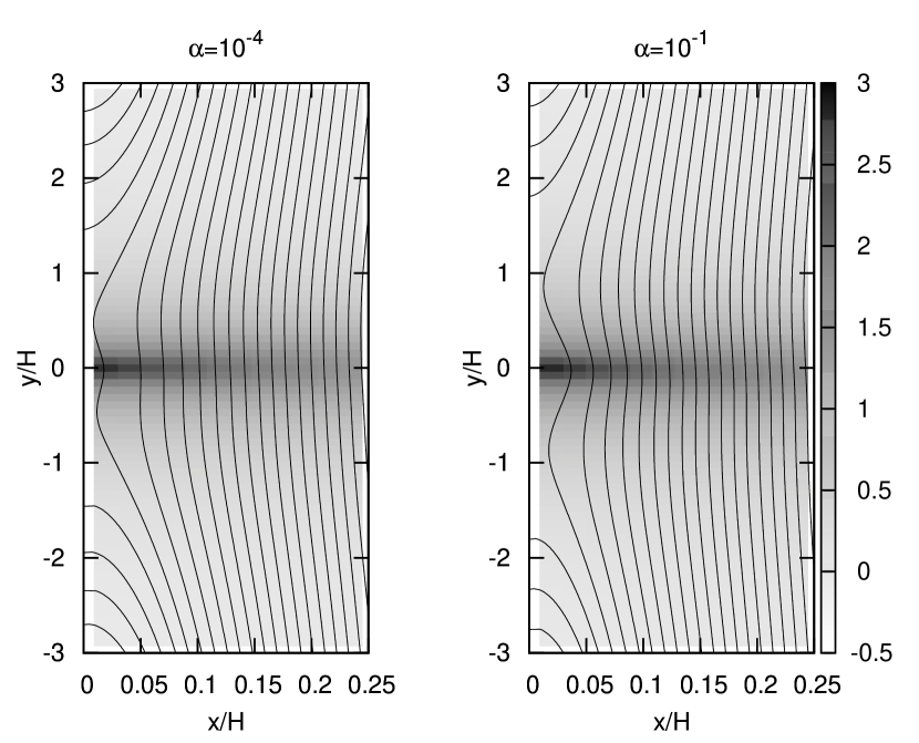
Figure 12: Density and streamline for calculations restricted to 2D mode in 3D calculation with $\alpha=10^{-4}$ (left) and $\alpha=10^{-1}$ (right). This corresponds to the calculations presented in Figure 4. Mass ratio between the central star $q=M_{\rm p}/M_{\rm c}$ and disk aspect ratio $h=H/r_{p}$ are assumed in such a way that $q/h^{3}=0.0252$, which is the same as Paardekooper and Papaloizou (2009b). Gray scale shows the density perturbation $\delta\rho/\rho_{0}$ divided by $q/h^{3}$ and solid lines are streamlines.

Figure 12 shows the streamlines plotted over the density fluctuations for calculations corresponding to Figure 4. Results with $\alpha=10^{-4}$ and $\alpha=10^{-1}$ are shown. Calculations are restricted to 2D modes of 3D calculation. Mass ratio between the planet and the central star $q=M_{\rm p}/M_{\rm c}$ and disk aspect ratio $h=H/r_{\rm p}$ are assumed in such a way that $q/h^{3}=0.0252$, just as Paardekooper and Papaloizou (2009b).

We find that the width of horseshoe orbit is $\sim 0.1H$ for $\alpha=10^{-4}$, while the width becomes slightly narrower in calculations with $\alpha=10^{-1}$. We have obtained about a factor of two smaller horseshoe width compared to Paardekooper and Papaloizou (2009b) in calculations with small viscosity (see Figure 3 of their paper.) We think that this is probably because we have weaker potential in the vicinity of the planet because of the effective softening introduced by vertical averaging, see equation (31). In Paardekooper and Papaloizou (2009b), they also obtained narrower horseshoe width in calculations with larger softening parameters. However, since we have neglected axisymmetric modes and non-linear effects, which may be potentially important in determining the streamline, this issue needs further investigation.

5.4 Axisymmetric Modes

Although we have neglected the axisymmetric modes in our calculations, a viscous overstability in axisymmetric modes has been discussed, especially in the context of Saturn’s rings. In this subsection, we discuss whether this overstability affects our results.

Local linear analysis of viscous overstability using a simple hydrodynamic model is performed by Schmidt et al. (2001). Stability criterion for isothermal case depends on the derivative of viscous coefficient $\nu$ with respect to surface density perturbation. We note that the system of equations we have solved, equations (20)-(23), are actually stable against viscous overstability, since our assumption of viscosity corresponds to $\beta=-1$ of Schmidt et al. (2001). In this case, we do not expect viscous overstability to occur and therefore, we can safely neglect the axisymmetric modes.

However, disk may be prone to viscous overstability if different prescription of viscosity is taken into account. If the non-linear consequence of viscous overstability produces non-axisymmetric structure in the vicinity of the planet, this may exert additional torque onto the planet. However, observation of the particle simulation performed by Schmidt et al. (2001) (their Figure 1 for example) indicates that non-axisymmetric modes are not strongly driven by the viscous overstability and therefore this may not play an important role in planetary migration. Nonetheless, the effects of viscous overstability seems to be an interesting extension of the analysis presented here.

5.5 Turbulent Disk

In this subsection, we briefly discuss that our analysis may indicate that the stochastic torque is important in a turbulent disk dominated by magneto-rotational instability (see e.g., Nelson and Papaloizou 2004). The effective turbulent viscosity originated in MRI may become as much as $\alpha\sim 0.1$ (e.g., Sano et al. 2004). Therefore, our calculation indicates that the density structure around the planet is more important than the tidal wave launched at the effective Lindblad resonances. Since the density structure around the planet is turbulent in the vicinity of the planet, stochastic force may be exerted on the planet embedded in such a turbulent disk.

In order for the $\alpha$-viscosity prescription [see equation (27)] to be a good approximation of the turbulent flow, the length scale in consideration must be larger than the eddy size. In the present problem, the scale in consideration is smaller than disk thickness. In a turbulent flow driven by MRI, eddies of sizes on the order of several tenths of the disk scale lengths exist. This can be understood if we notice that the wavelength of the most unstable mode is much smaller than the scale height of the disk with weak magnetic field. If weak poloidal magnetic field, $B_{z0}$, is exerted on the unperturbed disk, there always exists a net magnetic flux,

$$\langle B_{z}\rangle=B_{z0},$$ (71)

where $\langle B_{z}\rangle$ is the horizontally averaged $z$-component of magnetic field. Therefore, there always exists eddies with scales of the order of the most unstable mode of magneto-rotational instability with net flux $B_{z0}$,

$$\lambda\sim{\displaystyle\frac{v_{A,0}}{\Omega}},$$ (72)

where $\lambda$ is the eddy scale, $v_{A,0}=B_{z0}/\sqrt{4\pi\rho}$ is Alfvén  velocity constructed from the average poloidal field, and $\Omega$ is Keplerian angular frequency. In most cases, Alfvén velocity is smaller than sound speed by more than an order of a magnitude,

$$v_{A,0}\mathrel{\hbox{\hbox to0.0pt{\hbox{\lower 4.0pt\hbox{$\sim$}}\hss}\hbox{$<$}}}10^{-1}c.$$ (73)

This indicates

$$\lambda\mathrel{\hbox{\hbox to0.0pt{\hbox{\lower 4.0pt\hbox{$\sim$}}\hss}\hbox{$<$}}}10^{-1}H.$$ (74)

Thus, we can possibly use the effective turbulent viscosity in order to study the qualitative effects of the interaction between a turbulent disk and a planet.

However, the effective values of $\alpha$ may be obtained by averaging turbulent stress over several scale heights, since it includes all sizes of eddy that is important in turbulent flow driven by MRI. Thus, the use of $\alpha$ prescription may not be valid in discussing very small scale structure, and full MHD calculation is necessary. More detailed, quantitative analyses require high-resolution numerical study of the magnetized turbulent disk.

We have found that the effects of viscosity becomes apparent if $\alpha$ exceeds the value of $\sim 0.01-0.1$. Actual values of $\alpha$ in the disk is largely uncertain, but estimated values are around this value. Numerical simulations by Sano et al. (2004) indicates that the values of $\alpha$ varies from $10^{-4}-10^{-1}$ depending on the setup. From the observational constraints of dwarf novae, which seem to be better studied than protoplanetary disks, it is indicated that the values of $\alpha$ can vary from $0.01$ to $0.1$ (e.g., Cannizzo et al. 1988). The values of $\alpha$ seems to be an open issue for both theoretically and observationally.

Figure 1: Comparison of the torque obtained in 2D calculation and the 2D mode of 3D calculation for various $L_{z}$. In 2D calculations (dashed line), we use the gravitational potential given by equation (29), while in 2D mode of 3D calculation (solid line), we use the gravitational potential given by equation (31). The value of the normalized torque, $T/\Gamma_{\rm 2D}$ is plotted, where $\Gamma_{\rm 2D}$ is defined by equation (32).

Figure 2: Comparison of the 2D mode of the potential used by Tanaka et al. (2002) given by equation (33) (solid line) and the $k_{z}=0$ mode of the potential given by (31) with $L_{z}=2.7H$ (dashed line).

Figure 3: Variation of torque as a function of viscous coefficient $\alpha$ as a result of 3D calculation restricted to 2D modes.

Figure 4: Contour plot of the density fluctuation $\delta\rho/\rho_{0}$ around the planet (located at the origin) for 2D mode of 3D calculation with $L_{z}=2.5H$ with $\alpha=10^{-4}$ (left) and $\alpha=10^{-1}$ (right). Axisymmetric mode is not included.

Figure 5: Torque density given by equation (26) for $\alpha=10^{-4}$ (solid line) and $\alpha=10^{-1}$ (dashed line). Values are normalized according to equation (36).

Figure 6: Forward-back asymmetry of the torque distribution given by equation (37) for $\alpha=10^{-4}$ and $\alpha=10^{-1}$.

Figure 7: Variation of the torque as a function of viscosity parameter $\alpha$ obtained for 3D calculations (plus). For comparison, we plot the results restricted to 2D modes by cross. Dashed line shows the fitting function given by equation (38).

Figure 8: Torque density profile obtained by 3D calculation with various $\alpha$. Solid line shows the results of $\alpha=10^{-4}$, thick dashed line $\alpha=10^{-2}$, and thick dotted line $\alpha=10^{-1}$.

Figure 9: The contour plot of 3D mode density structure in $yz$-plane at $x=0.068H$ with $\alpha=10^{-4}$ (solid line) and $\alpha=10^{-1}$ (dashed line). The lines show the contours of $\delta\rho/\rho_{0}=10$.

Figure 10: One-sided torque obtained by 3D calculation for different smoothing length. Horizontal axis shows the values of smoothing length $\epsilon_{\rm 3D}$ and vertical axis shows the one-sided torque. Calculations with $\alpha=10^{-4}$ (solid line) and $10^{-1}$ (dashed line) are shown.

Figure 11: One-sided torque obtained by 3D calculation for different grid resolutions. Horizontal axis shows the values of grid size (the same for all three dimensions) and vertical axis shows the one-sided torque. Softening parameter $\epsilon_{\rm 3D}=10^{-3}H$ is used. Calculations with $\alpha=10^{-4}$ (solid line) and $10^{-1}$ (dashed line) are shown.

References

- Artymowicz (1993) Artymowicz, P., 1993 ApJ, 419, 155
- Balbus & Hawley, (1991) Balbus, S. A., & Hawley, J. F., 1991, ApJ, 376, 214
- Baruteau & Masset, (2008) Baruteau, C., & Masset, F., 2008, ApJ, 672, 1054
- Cannizzo et al., (1988) Cannizzo, J. K., & Shafter, A. W., & Wheeler, J. C., 1988, ApJ, 333, 227
- D’Angelo et al. (2002) D’Angelo, G., Henning, T., & Kley, W., 2002, A&A, 385, 647
- D’Angelo et al. (2003) D’Angelo, Kley, W., & Henning, T., 2003, ApJ, 586, 540
- Fromang et al. (2005) Fromang, S., Terquem, C., & Nelson, R.P., 2005, MNRAS, 363, 943
- Goldreich and Lynden-Bell (1965) Goldreich, P., & Lynden-Bell, D., 1965, MNRAS, 130, 125
- Goldreich & Tremaine, (1979) Goldreich, P., & Tremaine, S., 1979, ApJ, 233, 857
- Goodman and Rafikov (2001) Goodman, J., & Rafikov, R. R., 2001, ApJ, 552, 793
- Korycansky & Pollack, (1993) Korycansky, D. G., & Pollack, J. B., 1993, Icarus, 102, 150
- Masset (2001) Masset, F. S., 2001, ApJ, 558, 453
- Masset (2002) Masset, F. S., 2002, A&A, 387, 605
- Meyer-Vernet & Sicardy, (1987) Meyer-Vernet, N., & Sicardy, B., 1987, Icarus, 69, 157
- Muto et al. (2008) Muto, T., Machida, M. N., & Inutsuka, S.-i., 2008, ApJ, 679, 813
- Narayan et al. (1987) Narayan, R., Goldreich, P., & Goodman, J., 1987, MNRAS, 228, 1
- Nelson & Papaloizou, (2004) Nelson, R. P., & Papaloizou, J. C. B., 2004, MNRAS, 350, 849
- Paardekooper and Mellema (2008) Paardekooper, S.-J., & Mellema, G., 2006, A&A, 459, L17
- Paardekooper and Papaloizou (2008) Paardekooper, S.-J., & Papaloizou, J. C. B., 2008, A&A, 485, 877
- (20) Paardekooper, S.-J., & Papaloizou, J. C. B., 2009a, MNRAS, 394, 2283
- (21) Paardekooper, S.-J., & Papaloizou, J. C. B., 2009b, MNRAS, 394, 2297
- Papaloizou & Lin, (1984) Papaloizou, J. C. B., & Lin, D. N. C., 1984, ApJ, 285, 818
- Press et al. (1992) Press, W. H., Flannery, B. P., Teukolsky, S. A., & Vetterling, W. T., 1992, Numerical Recipes in Fortran 90: The Art of Scientific Computing , (Cambridge: Cambridge Univ. Press)
- Sano et al. (2004) Sano, T., Inutsuka, S.-i., Turner, N. J., & Stone, J. M., 2004, ApJ, 605, 321
- Schmidt et al. (2001) Schmidt, J., Salo, H., Spahn, F., & Petzschmann, O., 2001, Icarus, 153, 316
- Takeuchi et al. (1996) Takeuchi, T., Miyama, S. M., & Lin, D. N. C., 1984, ApJ, 460, 832
- Tanaka et al. (2002) Tanaka, H., Takeuchi, T., & Ward, W. R., 2002, ApJ, 565, 1257
- Terquem (2003) Terquem, C. E. J. M. L. J., 2003, MNRAS, 341, 1157
- Ward (1986) Ward, W. R., 1986, Icarus, 67, 164
- Ward (1989) Ward, W. R., 1989, ApJ, 336, 526