A new formal solution of the radiative transfer in arbitrary velocity fields.

Abstract

Aims. We present a new formal solution of the Lagrangian equation of radiative transfer that is useful in solving the equation of radiative transfer in the presence of arbitrary velocity fields.

Methods. Normally a term due to the inclusion of the wavelength derivative in the Lagrangian equation of radiative transfer is associated with a generalised opacity. In non-monotonic velocity fields, this generalised opacity may become negative. To ensure that the opacity remains positive, this term of the derivative is included in the formal solution of the radiative transfer problem.

Results. The new definition of the generalised opacity allows for a new solution of the equation of radiative transfer in the presence of velocity fields. It is especially useful for arbitrary velocity fields, where it effectively prevents the occurrences of negative generalised opacities and still allows the explicit construction of the $\Lambda$-operator of the system needed for an accelerated $\Lambda$-iteration. We performed test calculations, where the results of old, established solutions were compared with the new solution. The relative deviations never exceeded 1 % and so the new solution is indeed suitable for use in radiative-transfer modelling.

Non-monotonic velocity fields along photon paths frequently occur in three-dimensional hydrodynamical models of astrophysical atmospheres. Therefore, the formal solution will be of use for multidimensional radiative transfer and has immediate applications in the modelling of pulsating stars and astrophysical shock fronts.

1 Introduction

The Lagrangian equation of radiative transfer for moving atmospheres (Mihalas 1980) has been successfully solved for different astrophysical atmospheres, in particular supernova and nova atmospheres, as well as stellar atmospheres with winds.

The inclusion of velocity fields in the equation of transfer gives rise to two terms, one which is proportional to the specific intensity. This term is of the same form as the term arising from the opacity. Thus, the term from the velocity field can be included in the definition of a generalised opacity (see for instance Hauschildt 1992). For positive, velocity gradients, the contribution of the velocity field to the generalised opacity is always positive. In the case of negative, velocity gradients, the velocity field contribution may become dominant and produce a negative, generalised opacity. Thus, the method of solution must avoid exponentially increasing terms in the formal solution because such terms make the numerical computation unstable.

We show how to avoid this problem by not introducing a generalised opacity but instead including the velocity field in the formal solution of the radiative transfer. Negative opacity will occur in non-monotonic velocity fields, thus any numerical scheme for the formal solution must be able to handle both positive and negative velocity gradients. Numerically, the formal solution of the radiative transfer problem is then no longer an initial-value problem but a boundary-value problem. A formal solution of this situation was described by Baron & Hauschildt (2004) and the revised formal solution in this paper is derived from that solution. In addition, the formal solution incorporates the two discretisation schemes for the wavelength derivative and their mixing described by Hauschildt & Baron (2004). It it important to note that the new formal solution must be consistent with the solution to the scattering problem, e.g. an Accelerated $\Lambda$-iteration (ALI) (Scharmer 1981) as used in this work.

An immediate application of this new solution is to both one-dimensional model atmospheres of pulsating giant stars and shock fronts of all kinds, such as the interaction of a supernova envelope with the interstellar medium producing both forward and reverse shocks. In the course of multidimensional modelling of astrophysical flows, the use of these solutions will become unavoidable since arbitrary velocity fields occur frequently, due to e.g. Rayleigh-Taylor instabilities. In fact it is impossible to perform comoving radiative transfer in arbitrary velocity fields by means of a characteristic method without the use of a formal solution that totally avoids the occurrence of negative generalised opacities.

We derive the revised formal solution with a different definition of the opacity in Sect. 2. In Sect. 3, we demonstrate that this solution produces results consistent with established solutions and present brief conclusions in Sect. 4.

2 The construction of the formal solution

We solve the equation of radiative transfer by following the solution along characteristic rays. In this form, the transport of the specific intensity $I$ is described along a photon path (with path length $s$) and is independent of the dimensionality of the underlying atmosphere:

$$\frac{\mathrm{d}I_{\lambda}}{\mathrm{d}s}=\eta_{\lambda}-\chi_{\lambda}I_{\lambda}-4a_{\lambda}I_{\lambda}-a_{\lambda}\frac{\partial(\lambda I_{\lambda})}{\partial\lambda},$$ (1)

where $\eta$ is the emissivity and $\chi$ is the total extinction opacity. The dependence on the comoving wavelength has been explicitly separated from the differential $\frac{\mathrm{d}}{\mathrm{d}s}$ $\lambda$ giving rise to the $4a_{\lambda}I_{\lambda}$ term that can be incorporated into a generalised opacity. The term $a_{\lambda}=\frac{\partial\lambda}{\partial s}$ is due to the wavelength coupling and is, for instance, given in spherical symmetry by:

$$a_{\lambda}=\gamma\left(\gamma^{2}\mu(\mu+\beta)\frac{\partial\beta}{\partial r}+\frac{\beta(1-\mu^{2})}{r}\right),$$ (2)

where $\beta=v/c$, $\gamma=1/\sqrt{1-\beta^{2}}$, and $r$ and $\mu=\cos{\vartheta}$ are the phase-space coordinates (wavelength is of course a phase-space coordinate). We note that it is the sign of the wavelength-coupling term, and not the sign of the velocity gradient, that determines the upwind sense of the wavelength derivative.

The form of Eq. 1 is the same for all geometries and dimensionalities. However, the form of the differential $\frac{\mathrm{d}}{\mathrm{d}s}$ and the coupling term $a_{\lambda}$ will differ.

To formally solve Eq. 1, the wavelength derivative $\frac{\partial(\lambda I)}{\partial\lambda}$ must be discretised. We adopt the notation of Hauschildt & Baron (2004), where two possible discretisations of the wavelength derivative are combined in a Crank-Nicholson-like scheme.

Since we allow for arbitrary velocity fields, the formal solution must allow for an arbitrary sense of wavelength derivative that is, the upwind direction may correspond either to longer or shorter wavelengths. To insure the stability of the discretisation, local upwind schemes are introduced (Baron & Hauschildt 2004) depending on the coupling term $a_{\lambda}$. We assume a sorted wavelength grid $\lambda_{l-1}<\lambda_{l}<\lambda_{l+1}$, and the wavelength dependence is represented by the wavelength index. The wavelength derivative can then be written as:

$$\frac{\partial(\lambda_{l}I_{l})}{\partial\lambda}=\left\{\begin{array}[]{l}\displaystyle\frac{\lambda_{l}I_{l}-\lambda_{l-1}I_{{l-1}}}{\lambda_{l}-\lambda_{l-1}}\,\displaystyle\mathrm{:}\,a_{\lambda_{l}}\geq 0\\ \displaystyle\frac{\lambda_{l}I_{l}-\lambda_{l+1}I_{{l+1}}}{\lambda_{l}-\lambda_{l+1}}\,\displaystyle\mathrm{:}\,a_{\lambda_{l}}<0\end{array}\right\}=\left[p_{l}^{-}I_{{l-1}}+p_{l}^{|}I_{l}+p_{l}^{+}I_{{l+1}}\right]$$

where the $p_{l}^{\bullet}$ are defined as:

$$\left.\begin{array}[]{l}\displaystyle p_{l}^{-}=\displaystyle-\frac{\lambda_{l-1}}{\lambda_{l}-\lambda_{l-1}}\\ \displaystyle p_{l}^{|}=\displaystyle\phantom{-}\frac{\lambda_{l}}{\lambda_{l}-\lambda_{l-1}}\\ \displaystyle p_{l}^{+}=\displaystyle\phantom{-}0\end{array}\right\}a_{\lambda_{l}}\geq 0,\quad\left.\begin{array}[]{l}\displaystyle p_{l}^{-}=\displaystyle\phantom{-}0\\ \displaystyle p_{l}^{|}=\displaystyle\phantom{-}\frac{\lambda_{l}}{\lambda_{l}-\lambda_{l+1}}\\ \displaystyle p_{l}^{+}=\displaystyle-\frac{\lambda_{l+1}}{\lambda_{l}-\lambda_{l+1}}\end{array}\right\}a_{\lambda_{l}}<0$$ (3)

It should be noted that the $p_{l}^{\bullet}$ depend not only on wavelength but also on spatial position since the sign of the coupling term $a_{\lambda}$ may change along the characteristic.

For mixing parameters of $\xi\in[0,1]$ for the two different discretisations, the equation of radiative transfer then reads:

$$\frac{\mathrm{d}I_{l}}{\mathrm{d}s} = \eta_{l}-\chi_{l}I_{l}-a_{l}\left(4+\xi\;p_{l}^{|}\right)I_{l}-\xi\;a_{l}\left(p_{l}^{-}I_{{l-1}}+p_{l}^{+}I_{{l+1}}\right)$$ (4)

$$\;-[1-\xi]\;a_{l}\left(p_{l}^{-}I_{{l-1}}+p_{l}^{|}I_{l}+p_{l}^{+}I_{{l+1}}\right)$$

To solve Eq. 4 for monotonic velocity fields, it is customary to define a generalised opacity:

$$\hat{\chi}_{l}=\chi_{l}+a_{l}\left(4+\xi\;p_{l}^{|}\right)$$ (5)

This approach in general, however, often fails because the generalised opacity in Eq. 5 may become negative if:

$$-4a_{l}>\chi_{l}+a_{l}\xi\;p_{l}^{|}$$ (6)

(Note that the $p_{l}^{|}$ coefficient always has the same sign as $a_{l}$). For strong wavelength couplings — as for instance in shock flows — the condition 6 is easily fulfilled. To avoid negative optical depths along the characteristics, the generalised opacity must be defined differently. In the $\xi=1$ case, negative opacities could be eliminated by adopting a fine wavelength sampling anywhere apart from at the boundaries where the $p_{l}^{|}$ vanish. In principle, one could consider a method of correcting the formal solution at these points, but the corrections must then also be applicable to the explicit construction of the $\Lambda$-operator.

A positive generalised opacity is assured by the following definition:

$$\hat{\chi}_{l}=\chi_{l}+\xi\;a_{l}p_{l}^{|},$$ (7)

which only incorporates the physical opacity and a purely positive contribution from the velocity field. The remaining term $4a_{l}I_{l}$ must then be incorporated into the formal solution of the equation of radiative transfer. This term then has the same effect as if it was included in the opacity definition. For positive $a_{l}$, the contribution to the formal solution is negative and therefore decreases the intensity along the ray in a way similar to an increase in opacity provides. For negative $a_{l}$, the contribution is positive which behaves like a negative opacity. This new solution indeed provides identical results to the previous discretisation method (see Sect. 3).

After integrating Eq. 4 along a photon path from path length $s_{1}$ to $s_{2}$, the formal solution between two spatial points on a characteristic can then be written in terms of optical depth, since the optical depth $\tau_{\lambda}$ along the characteristic relates to the path length by means of $\mathrm{d}\tau_{l}=\hat{\chi}_{l}\mathrm{d}s$.

$$I_{l}(\tau_{2}) = I_{l}(\tau_{1})e^{\tau_{1}-\tau_{2}}+\int_{\tau_{1}}^{\tau_{2}}\!\!\!\hat{S}_{l}e^{\tau-\tau_{2}}\mathrm{d}\tau-\int_{\tau_{1}}^{\tau_{2}}\!\!\!\tilde{S}_{l}e^{\tau-\tau_{2}}\mathrm{d}\tau$$ (8)

where $\tau_{i}=\tau_{l}(s_{i})$ and

$$\hat{S}_{l} = \frac{\chi_{l}}{\hat{\chi}_{l}}\left(S_{l}-\xi\;\frac{a_{l}}{\chi_{l}}\left(p_{l}^{-}I_{{l-1}}+p_{l}^{+}I_{{l+1}}\right)\right)$$ (9)

$$\tilde{S}_{l} = \frac{a_{l}}{\hat{\chi}_{l}}\left([1-\xi]\;\left(p_{l}^{-}I_{{l-1}}+p_{l}^{+}I_{{l+1}}\right)+\left[4+[1-\xi]\;p_{l}^{|}\right]I_{l}\right)$$ (10)

In a discrete atmosphere model, the integrals in Eq. 8 can be evaluated by means of piecewise linear- or parabolic interpolation of the auxiliary source functions:

$$\int_{\tau_{i-1}}^{\tau_{i}}\hat{S}_{l}e^{\tau-\tau_{i}}\mathrm{d}\tau \approx \alpha_{i,l}\hat{S}_{i-1,l}+\beta_{i,l}\hat{S}_{i,l}+\gamma_{i,l}\hat{S}_{i+1,l}$$ (11)

$$\int_{\tau_{i-1}}^{\tau_{i}}\tilde{S}_{l}e^{\tau-\tau_{i}}\mathrm{d}\tau \approx \alpha_{i,l}\tilde{S}_{i-1,l}+\beta_{i,l}\tilde{S}_{i,l}$$ (12)

where the coefficients $\alpha$, $\beta$, and $\gamma$ are described in Olson & Kunasz (1987) and Hauschildt (1992). Note that the contribution from the explicit wavelength derivative has been only linearly interpolated, whereas the implicit part can also be parabolically interpolated.

The construction of the matrix equation for the formal solution as well as the analytic construction scheme for a $\Lambda$ operator described in Baron & Hauschildt (2004) can be used without modification in the new formal solution. These steps will therefore not be repeated here.

3 The test calculations

To compare the new solution with other solutions, we used a simplified test setup (see also Hauschildt & Baron (2004) and Knop et al. (2007)). The opacity consists of a grey continuum and a single atomic line. The continuum opacity $\chi_{\kappa}$ is grey and varies with the radial structure according to $\chi_{\kappa}\propto r^{-2}$. The expression $\chi_{\kappa}=\kappa_{\kappa}+\sigma_{\kappa}$ includes absorption $\kappa_{\kappa}$ as well as scattering $\sigma_{\kappa}$, which are related by a thermalisation parameter $\epsilon_{\kappa}=\kappa_{\kappa}/\chi_{\kappa}$. The corresponding opacities $\kappa_{\mathrm{line}},\sigma_{\mathrm{line}}$, and thermalisation $\epsilon_{\mathrm{line}}$ are used for the — assumed to be Gaussian shaped — spectral line of the two-level-atom, where its strength is parameterised relative to the continuum opacity $R=\chi_{\mathrm{line}}/\chi_{\kappa}$. The atmosphere has an extension of $r_{\mathrm{min}}<r<101\,$, where $r_{\mathrm{min}}=10^{13}\mathrm{cm}$. A radial optical-depth scale is mapped onto the radial grid with the continuum opacity and ranges from $10^{-6}<\tau<10^{4}$. To include wavelength couplings in the atmosphere, a velocity field is imposed on the radial structure.

At first, we checked that, for an absent velocity field, the old and new formal solutions provide identical results. Then we used monotonic velocity fields, in order to compare the new formal solutions with the well tested solution described in Hauschildt (1992). For the velocity field, a linear law $v(r)=v_{\mathrm{max}}\;r_{\mathrm{max}}/r$ with $v_{\mathrm{max}}=1000\mathrm{km}/\mathrm{s}$ was assumed.

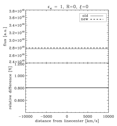
(a)

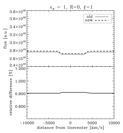
(b)

Figure 1: Comparison of the comoving spectra for the cases $\xi=0$ in (a) and $\xi=1$ in (b) where the new solution is represented by the black dashed line and the old one by the solid grey line. The wavelength scale is given in $km/s$ around a fictitious line center. The line is omitted and the continuum is purely absorptive.

In the upper panel of Fig. 1a, the comoving frame spectrum for a pure absorptive continuum without a line — $\sigma_{\kappa}=0$ and $R=0$ — is shown for $\xi=0$. The new solution is plotted with a dashed black line, while the old solution is represented by a solid grey line. The lower panel of Fig. 1a illustrates the difference between the two solutions, implying that both solutions reproduce the expected flat continuum and differ about 1%. For comparison, the computations in Fig. 1a were repeated for the case $\xi=1$ and are shown accordingly in Fig. 1b. The fully implicit $\xi=1$ wavelength discretisation had difficulties in reproducing a flat continuum because to its diffusive behaviour, as also demonstrated by Hauschildt & Baron (2004). This is also true for the new solution, as can be seen in the upper panel of Fig. 1b; the new formal solution closely follows the old solution, as is also evident in the lower panel of Fig. 1b. The relative difference never exceeds 1 %, which is less than the deviation of the continuum from flatness.

Since no scattering was included in the opacity, there is no need for an ALI and a single $\Lambda$-step will solve directly the system. The comparisons between the comoving spectra then directly yield the differences in the formal solutions.

In the next test, a scattering continuum opacity — of $\epsilon_{\kappa}=10^{-2}$ — was added, but the line was still omitted. The results for the case of $\xi=0$ are shown in Fig. 2a, and for $\xi=1$ in Fig. 2b with the same colour codes as before. The top panels show the comoving spectra and the relative differences are shown in the bottom panels. The differences between the scattering continua are of the order of only $10^{-3}$ %. The diffusive behaviour of the fully implicit solutions appears again in the deviations from a flat continuum.

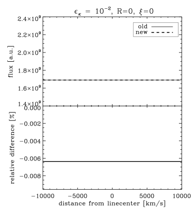
(a)

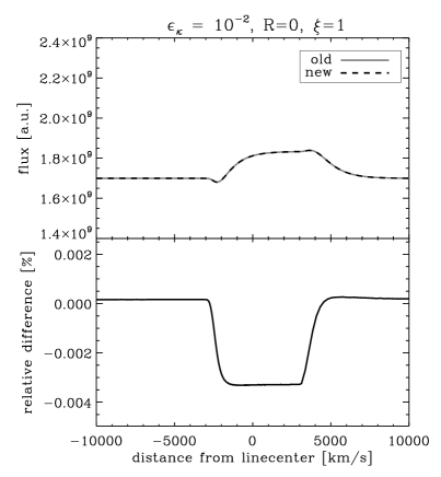
(b)

Figure 2: Same as in Fig. 1, apart from the fact that the spectral line is omitted and the continuum has a thermalisation parameter of $\epsilon_{\kappa}=10^{-2}$.

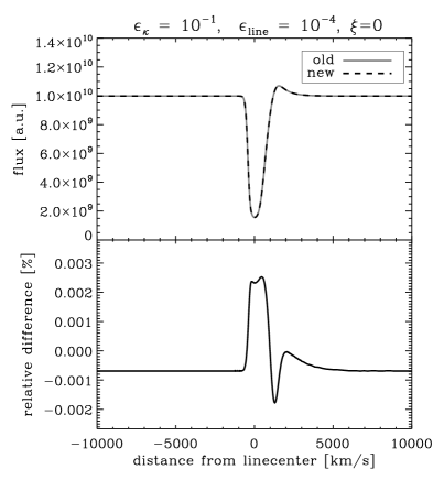
(a)

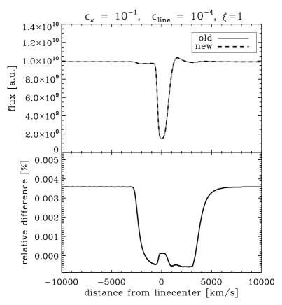
(b)

Figure 3: Same as in Fig. 1, apart from the fact that the spectral line is strongly scattering ($\epsilon_{\mathrm{line}}=10^{-4}$) and the continuum has a thermalisation parameter of $\epsilon_{\kappa}=10^{-1}$.

In further tests, a strong scattering line — with $R=100$ and $\epsilon_{\mathrm{line}}=10^{-4}$ — was added to the continuum opacity which is also affected by additional scattering — $\epsilon_{\kappa}=10^{-1}$. The results for the $\xi=0$ discretisation are shown in Fig. 3a. The upper panel again shows the comoving spectrum with the new solution in dashed black and the old solution in solid grey. The resulting line profile is a typical scattering line in an expanding atmosphere. The apparent excellent match of the two solutions is verified by the plot of the relative differences in the lower panel of Fig. 3a. The maximal difference is of the order of $10^{-3}$ %.

The same calculation has been performed for the $\xi=1$ weighted wavelength discretisation. The results are shown in Fig. 3b with the same colour codes as before. The comoving spectra show a disturbed continuum in the transition region between the line and the continuum, which can again be attributed to the more diffusive behaviour of this wavelength discretisation. However, again the match between the new and the old solution is excellent.

The excellent agreement between the old and new comoving spectra in the presence of scattering — with relative differences of the order of $10^{-3}$ % — may at first seem unusual because the differences in the formal solution itself were of the order only of one percent (see Figs. 1a and 1b). However, in these cases, no ALI was needed due to the lack of scattering. In the scattering cases, an ALI was performed. Since only exact elements from the $\Lambda$-operator have been used in the construction of the $\Lambda^{\ast}$-operator, the operators derived from the old and new formal solutions also differ. From the excellent agreement of the final results, it is obvious that these differences cancel each other and enable far closer agreement for the moments of the radiation field in the ALI than the formal solution for a given source function.

In the preceding tests, there was no need to employ the new solution because the velocity fields were monotonic. To test the new solution for alternating wavelength couplings, a non-monotonic, alternating velocity field was used.

To demonstrate the robustness of the new solution, we performed calculations for an alternating velocity profile — shown in Fig. 4 — that penetrates into the deep layers of the atmosphere. This run of the velocity profile was not even remotely possible within the old framework, and hence no comparison with the old solution is shown. The comoving spectrum is shown in Fig. 5. The peculiar features and broadness of the line result from the extreme velocity fields in the atmosphere. The $\xi=1$ discretisation had to be used, since the formal solution was ill-conditioned in the $\xi=0$ case.

This calculation was not intended to model a physical atmosphere. It instead was intended to demonstrate the robustness of the new solution for even extreme wavelength-coupling conditions.

Figure 4: Alternating velocity field in terms of optical depth.

Figure 5: Co-moving spectrum for the presence of the non-monotonic velocity field shown in Fig. 4 for $\xi=1$. The wavelength scale is given in $km/s$ around a fictitious line center. The line is strongly scattering ($\epsilon_{\mathrm{line}}=10^{-4}$) and the continuum has a thermalisation parameter of $\epsilon_{\kappa}=10^{-2}$.

We note that the removal of the $4a_{l}I_{l}$ term from the opacity and its addition as an explicit source term has apparently little influence on the solution. In all of our test calculations, all differences with respect to established solutions were minor. In the case of scattering in the line as well as in the continuum the differences become almost negligible. In comparison, the different discretisations had a far more dominant effect on the solution than the addition of the explicit term, as can be seen in the case of the $\xi=1$ weighting for which the diffusive behaviour is traced out. We should note further that the speed of convergence of the formal solution did not change significantly.

The new solution method appears to be well suited to general radiative-transfer modelling involving non-monotonic velocity fields. This has immediate applications to 1D spherical symmetric atmosphere models, e.g. for pulsating atmospheres of variable stars as well as shock fronts in supernova flows.

It remains to be seen whether the different numerical nature of the solution, due to an additional explicit term, will be troublesome in some cases. Our test computations did not identify an example of numerically unstable behaviour during the exploration of the parameter space.

4 Conclusions

We have presented a new formal solution of the equation of radiative transfer. Its advantage with respect to established solutions lies in the avoidance of negative opacities that occur by design in non-monotonic velocity fields. It allows the computation of the arbitrarily wavelength-coupled, radiative-transfer equation that arises with complete avoidance of negative, generalised opacities that render the solution unstable. The new approach is required for any modelling that involves alternating wavelength couplings. Since one considers radiative transfer in multidimensional situations, non-monotonic velocity fields do naturally occur.

The relative differences between the new and old solutions was not found to exceed 1 % in all test calculations and were in most cases several orders of magnitude smaller. Therefore, the new solution is a viable replacement of the old solutions and useful in modelling the atmospheres of variable stars or radiative transfer in hydrodynamically obtained structures.