Orientation-dependent spontaneous emission rates of a two-level quantum emitter in any nanophotonic environment

Abstract

We study theoretically the spontaneous emission rate of a two-level quantum emitter in any nanophotonic system. We derive a general representation of the rate on the orientation of the transition dipole by only invoking symmetry of the Green function. The rate depends quadratically on orientation and is determined by rates along three principal axes, which greatly simplifies visualization: Emission-rate surfaces provide insight on how preferred orientations for enhancement (or inhibition) depend on emission frequency and location, as shown for a mirror, a plasmonic sphere, or a photonic bandgap crystal. Moreover, insight is provided on novel means to ”switch” the emission rates by actively controlling the orientation of the emitters’ transition dipole.

I Introduction

It is well-known that the characteristics of spontaneously emitted light depend strongly on the environment of the light source Drexhage70 ; Kleppner81 ; Haroche92 ; Novotny06 . According to quantum electrodynamics, the emission rate of a two-level quantum emitter, described by Fermi’s golden rule, is generally factorized into a part describing the sources intrinsic quantum properties and another part describing the influence of the environment on the light field. Currently, there are many efforts to control the emission rate of quantum emitters by optimizing the nanoscale environment by, e.g., reflecting interfaces Drexhage70 ; Snoeks95 , microcavities Gerard98 ; Englund05 , photonic crystals Yab87 ; Sprik96 ; Lodahl04 ; Busch&John98 , or plasmonic nanoantennae Farahani05 ; Muskens07 ; Tam08 . Control of spontaneous emission is notably relevant to applications, including single-photon sources for quantum information, miniature lasers and light-emitting diodes, and solar energy harvesting Graetzel01 ; San02 ; Park04 .

The effect of the environment of a source on its emission rate is described by the local density of optical states (LDOS) Sprik96 ; Busch&John98 ; Novotny06 . The LDOS counts the number of photon modes available for emission, and it is interpreted as the density of vacuum fluctuations. In many experimentally relevant cases, it is theoretically known that emission rates strongly differ for various orientations of the transition dipole moment see, e.g., Novotny06 ; Kuhn2008 . Thus, the widely pursued control of position and frequency leaves a large uncertainty in the emission rate Sprik96 . To date, no clear picture has emerged of the general characteristics of the orientation dependence. It is an open question whether the behavior mimics the local symmetry around the emitter, see Fig. 1, or whether any generic dependence exists at all.

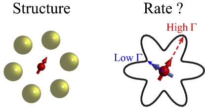
Figure 1: (color online) Drawing of a two-level quantum emitter embedded in an arbitrary nanophotonic system, here depicted as a cluster of 6 scatterers. If the emission rate were to mimic the symmetry of the system, one would here expect an emission-rate surface with a 6-fold symmetry. Our analysis reveals, however, that these surfaces take on only specific shapes determined by the symmetry of the Green dyadic. The symmetry analysis allows one to conclude without any calculation that the rate is identical for all dipole orientations in the plane of the 6 scatterers.

Therefore, we present fundamental insights in the complex dependence of the emission rates of a quantum emitter on the orientation of its dipole moment. Our general, yet simple theoretical analysis only invokes the symmetry of the Green function and provides a complete classification of the orientation-dependences that the emission rate can assume in any nanophotonic system. This classification leads to an intuitive visualization that is based on only a few clearly defined physical parameters, as shown by examples of an emitter near a mirror, a plasmonic sphere, or in a 3D photonic bandgap crystal. From our analysis, we conclude that control over the orientation of the transition dipole moment opens novel applications: If one can tune the orientation of an emitter, one can ”switch” emission from inhibited to enhanced and vice versa. In the field of quantum information Kimble08 , atomic qubits that fly by nanophotonic systems could acquire controllable phase shifts by tuning their orientation relative to the principal axes.

II Theory

II.1 Derivation of emission-rate surface

The rate of spontaneous emission $\Gamma$ of a two-level dipolar quantum emitter in the weak-coupling approximation is equal to Sprik96 ; Busch&John98 ; Novotny06 :

$$\Gamma(\omega,\mathbf{r},\mathbf{e}_{d})=\frac{\pi d^{2}\omega}{\hbar\epsilon_{0}}N(\mathbf{r},\omega,\mathbf{e}_{d}),$$ (1)

with $\omega$ the emission frequency, $\mathbf{r}$ the source’s position, $\mathbf{e}_{d}$ the dipole orientation, $d$ the modulus of the matrix element of the transition dipole moment. $N(\mathbf{r},\omega,\mathbf{e}_{d})$ is the local density of optical states (LDOS) that equals:

$$N(\omega,\mathbf{r},\mathbf{e}_{d})=\frac{6\omega}{\pi c^{2}}(\mathbf{e}_{d}^{T}\cdot\mathrm{Im}(\mathbb{G}(\mathbf{r},\mathbf{r},\omega))\cdot\mathbf{e}_{d}),$$ (2)

with $\mathbb{G}(\mathbf{r},\mathbf{r},\omega)$ the Green dyadic Novotny06 . Eq. (1) reveals the well-known fact that the emission rate depends on the frequency and the position of the emitter. As is well known, Eq. (2) is also applicable to emission dynamics inside dissipative optical media. In such media, the imaginary part of the Green dyadic describes the total decay rate, i.e., the sum of the radiative decay rate and the rate of quenching induced by the environment. Hence, the results in this paper carry over straightaway to the decay dynamics of dipoles emitters in dissipative nanophotonic environments.

A didactic example to illustrate the dependence of emission rates on frequency, position and dipole orientation is that of a source near a perfect mirror, see Fig. 2(A), which can be understood from image dipole analysis Haroche92 ; Drexhage70 . The rate depends strongly on the dipole orientation $\mathbf{e}_{d}$: at small distances a dipole parallel to the mirror has a vanishing emission rate, which can be interpreted as due to destructive interference of the dipole with its oppositely oriented image. In contrast, a dipole perpendicular to the mirror has twice the unperturbed rate owing to constructive interference, as shown in Fig. 2(B). Clearly, the symmetry of this particular geometry implies that the parallel and perpendicular dipole orientations are ‘principal’ orientations along which the maximum and minimum rates are attained. At intermediate orientations the rate is a weighted average of the two rates.

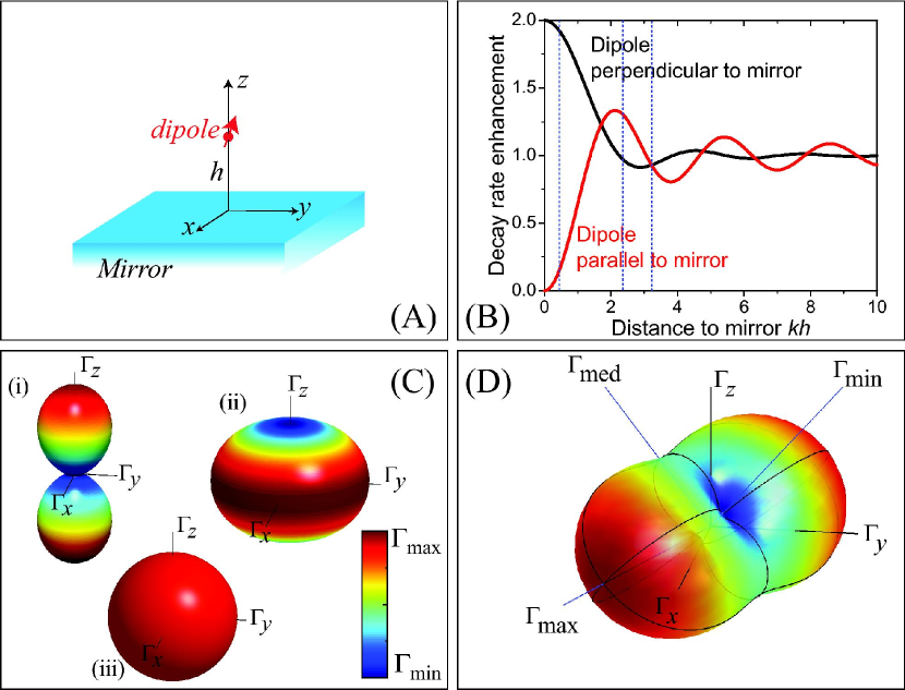
Figure 2: (color) (A) Drawing of a two-level quantum emitter at distance $h$ above a mirror. (B) Emission rate versus scaled distance (wave vector times distance $kh$) for a dipole perpendicular and parallel to a perfect mirror Haroche92 . (C) Three-dimensional surfaces representing the orientation dependent spontaneous emission rate in real space. (i) One maximal emission and two equal minimal rates give a peanut-shape (at $kh=0.4$ in (B)). (ii) Two equal maximal rates and one minimal rate give an oblate spheroid ($kh=2.3$ in (B)). (iii) Three equal maximal rates give a sphere ($kh=3.2$ in (B)). (D) Most general shape when all principal rates are different ($\Gamma_{\mathrm{max}}>\Gamma_{\mathrm{med}}>\Gamma_{\mathrm{min}}$) and the principal axes are rotated from the $(x,y,z)$-axes. Color scales are linear from $\Gamma_{\mathrm{min}}$ to $\Gamma_{\mathrm{max}}$ (colorbar in (C)).

The main result of our paper is that the rate always depends on orientation via a quadratic form with three perpendicular principal axes, as will now be proven: On account of reciprocity, the Green dyadic is equal to its transpose upon exchanging the coordinates. Hence

$$\mathrm{Im}(\mathbb{G}(\mathbf{r},\mathbf{r^{\prime}},\omega))^{T}=\mathrm{Im}(\mathbb{G}(\mathbf{r^{\prime}},\mathbf{r},\omega)).$$ (3)

Furthermore, the imaginary part of the Green dyadic is real. Therefore, the imaginary part of the Green dyadic in Eq. (2) is a real and symmetric $3\times 3$ matrix. Consequently, at each frequency $\omega$ and spatial position $\mathbf{r}$, the imaginary part of the Green dyadic can always be diagonalized, and has 3 eigenvalues ($g_{1}$, $g_{2}$, $g_{3}$) that correspond to three orthogonal eigenvectors. Since the eigenvalues can be ordered by magnitude, we relabel the eigenvalues and the concomitant main axes as $\{\mathbf{v}_{\mathrm{min}},\mathbf{v}_{\mathrm{med}},\mathbf{v}_{\mathrm{max}}\}$. This basis corresponds to three perpendicular principal dipole orientations that vary with dipole location $\mathbf{r}$ and frequency $\omega$. In this orthonormal basis we express the dipole orientation unit vector $\mathbf{e}_{d}$ as:

$$\mathbf{e}_{d}=\beta_{1}\mathbf{v}_{\mathrm{min}}+\beta_{2}\mathbf{v}_{\mathrm{med}}+\beta_{3}\mathbf{v}_{\mathrm{max}},$$ (4)

where $\beta_{i}$ are coefficients that are constrained through $\beta_{1}^{2}+\beta_{2}^{2}+\beta_{3}^{2}=1$ to lie on a unit sphere, since $\|\mathbf{e}_{d}\|=1$. Clearly, the coefficients $\beta_{i}$ are functions of the dipole orientation: $\beta_{i}=\beta_{i}(\mathbf{e}_{d})=\mathbf{e}_{d}^{T}\cdot\mathbf{v}_{i}$.

Using Eqs. (1, 2), the emission rate $\Gamma$ can be expressed in emission rate coefficients $\Gamma_{i}$, which are the rates for dipole orientations parallel to the principal axes $\mathbf{v}_{\mathrm{i}}$, leading to:

$$\Gamma(\mathbf{e}_{d})=\beta_{1}^{2}(\mathbf{e}_{d})\Gamma_{\mathrm{min}}+\beta_{2}^{2}(\mathbf{e}_{d})\Gamma_{\mathrm{med}}+\beta_{3}^{2}(\mathbf{e}_{d})\Gamma_{\mathrm{max}}.$$ (5)

Equation (5) describes the emission-rate surface as a function of dipole orientation $\Gamma(\mathbf{e}_{d})$, which is a central result of our work. The emission rate coefficients $\Gamma_{i}$ are equal to:

$$\Gamma_{i}=\frac{\pi d^{2}\omega}{\hbar\epsilon_{0}}\frac{6\omega}{\pi c^{2}}(\mathbf{v}_{\mathrm{i}}^{T}\cdot\mathrm{Im}(\mathbb{G})\cdot\mathbf{v}_{\mathrm{i}})=\frac{\pi d^{2}\omega}{\hbar\epsilon_{0}}\frac{6\omega}{\pi c^{2}}g_{i},$$ (6)

and are via $\mathbb{G}$ functions of the frequency and the dipoles’ position: $\Gamma_{i}=\Gamma_{i}(\omega,\mathbf{r})$. Assuming known principal rates $\Gamma_{i}$, the emission-rate surface $\Gamma(\mathbf{e}_{d})$ is always a quadratic form on the unit sphere. Moreover only quadratic forms of signature $s=\sum(\mbox{sign}(\Gamma_{i}))=3$ can occur mathencyc , since emission rates are physically constrained to be positive for all orientations. Therefore, polar plots of the rate versus dipole orientation - henceforth called emission-rate surface - take on only specific shapes classified by the ratios of $\Gamma_{\mathrm{min}},\Gamma_{\mathrm{med}}$, $\Gamma_{\mathrm{max}}$, with three perpendicular symmetry axes, regardless of the nanophotonic system. We remark that while Eq. (5) may appear as the defining equation of an ellipsoid, the emission-rate surface is not an ellipsoid since the problem is not about calculating a level surface of Eq. (5), which would be equivalent to constraining $\beta_{i}$ to yield a fixed $\Gamma$ in Eq. (5), rather than constraining $\beta_{i}$ to the unit sphere. Our result that emission surfaces are always necessarily quadratic forms defies the intuition (as sketched in Fig. 1) that emission rates inherit the symmetry of the nanophotonic system.

Regarding the assumptions we require to arrive at the quadratic form for the emission rate surfaces, we note that we have assumed real dipole moment in Eq. (2) (following Ref. Novotny06 ) and that we used reciprocity to ensure real and symmetric $\mbox{Im}(\mathbb{G}(\mathbf{r},\mathbf{r}))$. In case of reciprocal media it is easy to show that our results are also valid for complex transition dipole moments, and not just for real dipole moments. Furthermore, if we assume a real dipole moment, it appears that our results are also valid for metamaterials that violate reciprocity, i.e., in case $\mbox{Im}(\mathbb{G}(\mathbf{r},\mathbf{r}))$ is not symmetric or even not diagonalizable. Since $\mbox{Im}(\mathbb{G}(\mathbf{r},\mathbf{r}))$ is still real it will nonetheless give rise to a quadratic form that can be transformed to a principal axis system mathencyc . The physical requirement that rates are positive for all dipole orientations furthermore ensures that the signature of the quadratic form remains $3$ even in the nonreciprocal case.

II.2 Generic shapes of the emission-rate surface

Figure 2(C,D) categorizes all possible shapes of the emission rate polar plot. Fig. 2(C) is relevant for the mirror, with principal axes parallel ($x,y$, degenerate) and perpendicular ($z$) to the interface. Fig. 2(C(i)) shows the emission-rate surface for the case where emission is enhanced along a single dipole orientation $\Gamma_{\mathrm{max}}\gg\Gamma_{\mathrm{min}}=\Gamma_{\mathrm{med}}$. This situation appears at a reduced distance $kh=0.4$ close to the mirror. Here, the emission-rate surface looks like a highly anisotropic peanut, constricted to a radius $\Gamma_{\mathrm{min}}$ in the $x,y$-plane, and extending to $\Gamma_{\mathrm{max}}$ along the $z$-axis. Fig. 2(C(ii)) shows the orientation dependent emission rate for a single inhibited axis with $\Gamma_{\mathrm{min}}\leq\Gamma_{\mathrm{med}}=\Gamma_{\mathrm{max}}$, at $kh=2.3$ near a mirror. Qualitatively, the emission-rate surface resembles an oblate spheroid; when the minimum rate is much less than the other two rates (see Fig. 5 below), the surface develops a concave indentation with a donut-like shape. Fig. 2(C(iii)) shows the emission-rate surface when the rate is equal along all three main axes ($kh=3.2$). The emission-rate surface is simply a sphere, as it is in any isotropic homogenous medium.

Fig. 2(D) shows the emission-rate surface for the most general case when i) the rates along the main axes are all different ($\Gamma_{\mathrm{min}}<\Gamma_{\mathrm{med}}<\Gamma_{\mathrm{max}}$), and ii) the principal axes $\mathbf{v}_{\mathrm{min,med,max}}$ have an arbitrary orientation with respect to the laboratory frame. Clearly, the emission rate is not extremal for a dipole parallel to any of the $(x,y,z)$-axes. An important feature of the emission-rate surfaces is that they allow for an easy inspection of both the anisotropy of the emission rates, and of the favorable dipole orientations compared to the usual $(x,y,z)$-axes in real space.

III Efficient method to calculate emission-rate surfaces

In many cases of practical interest, neither the Green’s function $\mathbb{G}$ nor the principal axes $\{\mathbf{v}_{\mathrm{i}}\}$ are a-priori known. Often algorithms based on a summation over all photon modes are used that only yield the rate $\Gamma$ for target orientations $\mathbf{e}_{d}$ chosen as a priori input. Reconstructing emission-rate surfaces as in Fig. 2 by a dense sampling of orientations is not viable with such algorithms, due to prohibitive computation times. A poignant example is the calculation of emission rates in photonic crystals that requires a summation over up to $10^{6}$ Bloch modes, the calculation of each of which requires diagonalization of a $10^{3}\times 10^{3}$ matrix, even for a single dipole orientation Busch&John98 ; Nikolaev09 . A popular alternative method that can conveniently yield the emission rate for a single orientation is the finite difference time domain (FDTD) simulation method FDTD . However, it appears difficult to calculate off-diagonal elements of the Green tensor. Since the various field components are not calculated on identical grid points, FDTD does not truly yield a Green dyadic on a well-defined position $\mathbf{r}$. Hence, even if an algorithm is known to calculate rates at fixed orientations, it is unclear how to find the principal axes and rates, since $\mbox{Im}(\mathbb{G})$ is simply not available for diagonalization. In view of the computational cost of evaluating the radiative rate at a single dipole orientation, the main problem is to find out for how many and for which orientations the emission rate must be calculated to completely and exactly characterize the emission-rate surfaces. Here we describe an efficient method to find principal emission rates and orientations by evaluating the LDOS at the least possible number of input orientations.

We use the well-known fact that any function on the unit sphere is conveniently expanded in spherical harmonics $Y_{lm}(\theta,\phi)=P_{lm}(\cos(\theta))e^{im\phi}$. Since the emission surface is a quadratic form, we can apply the well-known fact that all quadratic forms on the unit sphere can be represented exactly by an expansion containing only terms up to $l=2$, so that

$$\Gamma(\mathbf{e}_{d})=\sum_{l=0}^{2}\sum_{m=-l}^{l}a_{lm}P_{lm}(\cos(\theta))e^{im\phi}$$ (7)

An easy proof that no terms beyond $l=2$ are needed is obtained by expressing the spherical harmonics in terms of cartesian coordinates, rather than polar coordinates on the unit sphere mathencyc , or conversely by expressing the coefficients $\beta_{i}$ in terms of polar coordinates relative to the $\{\mathbf{v}_{\mathrm{i}}\}$ axis system. This substition leads to a trigonometric expansion for $\Gamma(\mathbf{e}_{d})$ with terms that are quadratic in cosines and sines of $\theta$ and of $\phi$, see Appendix A, Eq. (10).

The expansion coefficients for the spherical harmonic expansion are given by inner products

$$a_{lm}=\langle\Gamma(\mathbf{e}_{d}),Y_{lm}\rangle=\int_{0}^{2\pi}d\phi\int_{0}^{\pi}d\theta~{}\Gamma(\mathbf{e}_{d})Y_{lm}(\theta,\phi)\sin(\theta),$$ (8)

similar to the coefficients appearing in discrete Fourier transformations, but now for transformation on the unit sphere. Mohlenkamp has developed a fast Fourier transform method to calculate the coefficients numerically Mohlenkamp99 , which requires a sampling of rates $\Gamma$ at a discrete set of orientations, similar to the numerical evaluation of discrete Fourier coefficients by the sampling of a periodic function on a discrete set of points. In this approach, the integral expression (8) for the expansion coefficients for expanding a function $f$ is replaced by a discrete weighted sum:

$$\hat{a}_{lm}=\sum_{k}w_{k}f(\theta_{k},\phi_{k})Y_{lm}(\theta_{k},\phi_{k})\sin(\theta_{k}),$$ (9)

where $k$ runs over the finite set of sampling points. Such a discrete approximation to the expansion coefficients $a_{lm}$ is in fact exact for all functions $f$ that are exactly equal to a finite series of spherical harmonics up to order $l_{\mathrm{max}}$ if: i) the angles $(\theta_{k},\phi_{k})$ are chosen as the roots of the basis functions of order $l=l_{\mathrm{max}}+1$, and ii) the $w_{k}$ are appropriate weights. In the present case $l_{\mathrm{max}}=2$. Thus the special points are the 18 roots of the spherical harmonics $Y_{l,m}(\theta,\phi)$ of order $l=3$. Furthermore, one may appreciate that the spherical harmonic transform is a simple Fourier transform over $\phi$, and a Legendre transform over $\cos\theta$. The weights $w_{k}$ are hence the weights appropriate for Gauss-Legendre quadratures of order 3. Explicitly, the 18 special points occur at azimuthal angles $\phi=m\pi/3$ ($m=0,1,\ldots 5$) and at polar angles $\theta=\arccos(\sqrt{3/5}),\pi/2,\arccos(-\sqrt{3/5})$. The weights $w$ only depend on $\theta$, and are $5/9$ for $\theta=\arccos(\pm\sqrt{3/5})$ and $8/9$ for $\theta=\pi/2$. Since one half of the 18 points (see figure 3) is antipodal to the other half, inversion symmetry of the emission rate means that the rate need only be evaluated for 9 dipole orientations in order to find the full spherical harmonic expansion.

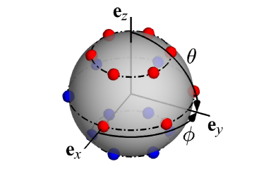
Figure 3: (color online) Special orientations, i.e., points on the unit sphere, for which the decay rate needs to be calculated in order to fully reconstruct emission-rate surfaces. The blue and red points together are the roots of $l=3$ spherical harmonics, corresponding to $\phi=m\pi/3$ ($m=0,1,2,\ldots 5$) and $\theta=\arccos(\sqrt{3/5}),\pi/2,-\arccos(\sqrt{3/5})$. Due to inversion symmetry, rates are equal for antipodal orientations. This makes calculations for half the points (e.g., the blue ones) superfluous, leaving 9 distinct orientations (red) for which rates must be calculated in order to find principal rates and orientations. Note that these points do not have equal weights in Eq. (9) (weight is $8/9$ for points on the equator and $5/9$ for other points).

IV Results for several nanophotonic examples

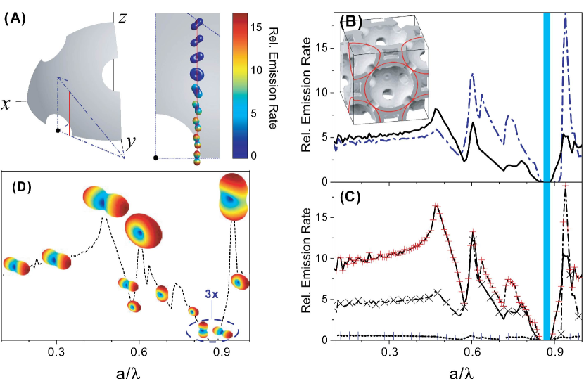
Figure 4: (color) Emission rate for a quantum emitter in a photonic bandgap crystal. (A) Left: $1/8$th of a cubic unit cell, blue dashed lines delimit the primitive cell. Right: emission-rate surfaces on $x=0.2$, $y=0.3$, variable $z$ (red line in left panel) at reduced frequency $a/\lambda=0.94$ ($a$ is lattice parameter). Surfaces are colored by relative rate (scalebar on right), and have constant size. (B) Emission rate for dipole centred in a window of a Si inverse opal [$\mathbf{r}=1/4(1,1,0)$, black dot in (A)] with orientations $\mathbf{e}_{d}=(1,0,0)$, $(0,1,0)$ (black curve), and $(0,0,1)$ (blue dashed-dotted curve) versus $a/\lambda$. The rate is normalized to the one in vacuum. The blue vertical bar indicates the photonic bandgap. Inset: cubic unit cell. (C) Maximum, medium, and minimum emission rates $\Gamma_{max}$ ($+$), $\Gamma_{med}$ ($\times$), $\Gamma_{min}$ ($|$) compared to rates for orientations $\mathbf{e}_{d}=(-1,1,0)/\sqrt{2}$ (full curve), $(0,0,1)$ (dashed-dotted), $(1,1,0)/\sqrt{2}$ (short dots). (D) Emission-rate surfaces at select frequencies show strong changes in shape. The size of the surfaces is in proportion to the absolute emission rates, and colorscales range from $\Gamma_{\mathrm{min}}$ to $\Gamma_{\mathrm{max}}$. Dashed curve: $\Gamma_{\mathrm{max}}$.

To illustrate our analysis, we discuss the emission dynamics of a quantum emitter inside a photonic crystal, illustrated in Fig. 4(A,B). These complex systems have extreme variations of the emission rate versus frequency on account of a bandgap where emission is completely inhibited Yab87 . To obtain the rate for an emitter of arbitrary orientation in a Si inverse opal, we have calculated the LDOS for the 9 special orientations by summing over all Bloch eigenmodes noteBloch . The crystal has a first order ‘pseudogap’ at reduced frequency 0.55, and a photonic bandgap from 0.852 to 0.891. Figure 4(B) shows the emission rate for a salient position in the unit cell (cf. Fig. 4(A)): the rate is anisotropic for frequencies near the pseudogap, since it differs for dipoles pointing in either $x,y$ or the $z$ direction, which are the cubic symmetry axes of the crystal. One might be tempted to perceive the behavior to be as simple as a mirror, since it is the same for both $x$ and $y$. However, a plot of the maximum, medium, and minimum emission rates (Fig. 4(C)) shows that this perception is completely wrong: Already at low frequency up to the pseudogap, the emission rate is strongly anisotropic. While anisotropic behavior in the long-wavelength limit may seem surprising, its origin in electrostatic depolarization effects has been discussed before Miyazaki98 ; Rogobete03 . The maximum rate occurs for dipole orientation $\mathbf{e}_{d}=(-1,1,0)/\sqrt{2}$, and is much larger than the rate for any of the $x,y,z$ orientations, whereas the minimum rate for $\mathbf{e}_{d}=(1,1,0)/\sqrt{2}$ is much smaller. At high frequency ($a/\lambda>0.6$) up to the bandgap, the orientation of maximum rate changes to $\mathbf{e}_{d}=(0,0,1)$. While it is clear from Fig. 4(C) that the orientation dependent emission rate is much more complex than expected from (B), Fig. 4(C) hardly gives an intuitive picture of the orientation-dependent behavior.

Therefore, we plot in Figure 4(D) emission-rate surfaces versus frequency. At frequencies below the pseudogap, the emission-rate surface is peanut-like, revealing that the emission rate is high for a ”horizontal” dipole orientation, and inhibited for the 2 perpendicular orientations. At the pseudogap, the emission-rate surface suddenly changes to donut-like, since the rate is high for two orientations and low for a third orientation. At even higher frequencies, the emission-rate surface becomes again peanut-like - with donut-like behavior near 0.8 - but with a different orientation than below the pseudogap. The maximum emission rate is up to 20-fold enhanced, and the anisotropy ($\Gamma_{\mathrm{max}}/\Gamma_{\mathrm{min}}$) is strong with peaks up to 340. In this particular example, the high symmetry at this spatial position fixes all principal axes. To demonstrate the applicability of our method to general, nonsymmetric, cases we have also studied low-symmetry positions at constant frequency, see Fig. 4(A). Again strong anisotropies occur, with the maximum-emission axis (or inhibition-axis) continuously changing direction as a function of source position. We conclude that emission-rate surfaces provide a compact representation of the rich behavior of the dependence of the emission rates on dipole orientation.

We emphasize that our classification of emission dynamics by means of emission-rate surfaces is by no means restricted to dielectric systems and can also be applied to dissipative nanophotonics systems that are of modern interest, such as plasmonic and metamaterial structures. Our analysis rests purely on the symmetry of the Green dyadic in Eq. (2), which in the presence of optical absorption describes the total decay rate (radiative rate plus induced nonradiative rate) of a quantum emitter. As an example, we discuss the textbook case of an emitter near a plasmonic sphere Anger06 ; Kuhn06 , using the known Green’s function Taibook (cf. Fig. 5(A)). Figure 5(C) shows that the emission-rate surface for the total decay rate has a donut-like shape ($\Gamma_{\mathrm{min}}\leq\Gamma_{\mathrm{med}}=\Gamma_{\mathrm{max}}$) with 16-fold enhanced rates for a dipole parallel to the surface, and 5-fold enhanced for a perpendicular dipole. For a fixed dipole orientation Novotny06 ; Kuhn2008 , the angular distribution of the radiated power reveals a well-known five-lobed structure (B). A comparison of (B) and (C) illustrates the main differences between radiation patterns and emission-rate surfaces: radiation patterns are relevant to a single dipole orientation and do not necessarily have any symmetry, or are free to follow any symmetry inherent in the environment. Emission-rate surfaces on the other hand are relevant to all orientations and have a symmetry limited by the quadratic form.

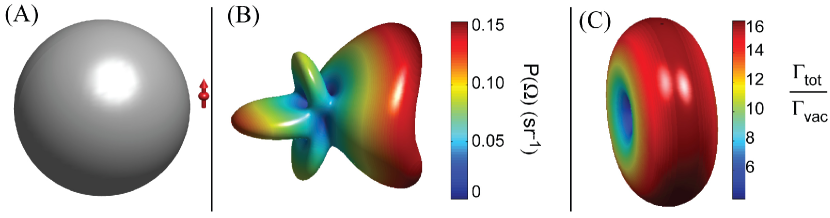
Figure 5: (color) (A) Drawing of a two-level quantum emitter at 20 nm distance from a plasmonic Ag sphere palik with radius $R=80$ nm. (B) Angular distribution of the radiated power versus solid angle $\Omega$ for a single dipole orientation parallel to the surface; the pattern has a complex five-lobed structure. (C) Emission-rate surface showing the emission rate versus dipole orientation. The pattern has a donut-like shape.

V Discussion

Since the analysis in this paper is based on $\mbox{Im}(\mathbb{G}(\mathbf{r},\mathbf{r}))$ it is strictly valid for the total decay rate modification induced by the nanophotonic environment. Explicitly, in the case of losses our proof only holds for the sum of the radiative rate and the non-radiative rate ($\Gamma_{\mathrm{rad}}+\Gamma_{\mathrm{nonrad}}$), and not for the radiative rate $\Gamma_{\mathrm{rad}}$ separately. To analyze the radiative emission-rate surfaces one would need to analyze the far-field integral of the radiated power (quantity in Fig. 5(B)) as a function of the source orientation. A priori it is not at all clear that such radiative rate surfaces need have a quadratic form. Indeed, we have not succeeded in proving the quadratic form for the radiative rate in the lossless case by analysis of far-field integrals, i.e., without identifying $\Gamma_{\mathrm{rad}}=\Gamma_{\mathrm{tot}}$ and subsequently analyzing $\mbox{Im}(\mathbb{G}(\mathbf{r},\mathbf{r}))$. We have numerically calculated radiative emission rate surfaces for many low-symmetry dissipative plasmon sphere clusters, and have not found any example in which the radiative emission rate surface was not quadratic. Although a rigorous proof is beyond the scope of this paper, we therefore anticipate that the quadratic form not only holds for total decay rates, but also for radiative decay rates.

A class of quantum emitters with a single transition dipole moment are fluorescent molecules, such as laser dyes Novotny06 . For such emitters, emission-rate surfaces can be observed if their orientation is controlled, e.g., by attaching them to liquid crystal molecules that are oriented in external fields Gottardo06 . If one can tune the orientation of an emitter, this opens a novel opportunity to ”switch” spontaneous emission from inhibited to enhanced and vice versa. The emission-rate surfaces reveal that optimal switching always requires a dipole rotation by $90^{\circ}$, since minimal and maximal emission rates always occur along the mutually perpendicular main axes. Alternatively, one could tune semiconductor nanowires with oriented dipole moments. For self-assembled and colloidal quantum dots with dipoles in a $x^{\prime},y^{\prime}$ plane, we expect to probe the $x^{\prime},y^{\prime}$ cross-sectional average of the emission-rate surface of the relevant nanophotonic system.

Since arbitrary orientations do not usually coincide with principal dipole orientations, most prior work on specific systems has been incomplete, since no principal rates has been reported. While such incompleteness does not affect the orientation averaged rate (see Appendix A), it does affect the understanding of dynamics of orientational dipole ensembles Gerard98 ; Lodahl04 ; Muskens07 . Such a decay is a sum of single exponentials with a rate distribution given by the emission-rate surface. Any observable derived from time-resolved decay beyond the orientation-averaged rate ($\mathrm{Tr}(\mathrm{Im}(\mathbb{G}))$) requires knowledge of the principal rates, which is thus relevant to many physical situations in nanophotonics.

In classical optics, the imaginary part of the Green dyadic is not only relevant for radiating dipoles. Indeed, the imaginary part of the Green dyadic has also been connected to the so-called coherency matrix (or the electric cross-spectral density tensor) MandelWolf95 for black body radiation. In general, the $3\times 3$ coherency matrix describes second-order spatial correlations of the electric field, and can be understood as a generalization of Stokes parameters to quantify the polarization of near fields locally. Within this framework, a description of local polarization by polarization ellipsoids directly points at a quadratic form of the coherency matrix, since ellipsoids are level sets (rather than polar plots) of an equation of the form in Eq. (5). It should be noted that the coherency matrix depends on the incident source that generates the local electric field. In the particular case that the field is due to black body radiation the coherency matrix reduces to the imaginary part of the Green dyadic $\mbox{Im}(\mathbb{G}(\mathbf{r},\mathbf{r}))$, as derived by Setälä et al. Setala03 . However, it is important to realize that for this identification of $\mbox{Im}(\mathbb{G}(\mathbf{r},\mathbf{r}))$ with the coherency matrix to hold, the source is required to be a statistically homogeneous and isotropic distribution of radiating currents, and the medium is supposed to be non-dissipative Setala03 . This is diametrically opposite to the analysis of spontaneous emission sources presented here, which concerns localized and oriented sources and is valid without limitation on material dissipation. It is exciting that our method to find principal rates and orientations can be directly adapted to calculate the local polarization properties of black body radiation.

VI Summary

We have theoretically studied the spontaneous emission rate of a two-level quantum emitter in any nanophotonic system. We derive a general representation of the dependence of emission rates on the orientation of the transition dipole by only invoking symmetry of the Green function. The rate depends quadratically on orientation and is determined by rates along three principal axes. We show that these principal rates and axes can be easily calculated without evaluation of the full Green function. Furthermore we show that visualization of emission-rate surfaces as determined from principal rates provides great insight on how preferred orientations for enhancement (or inhibition) depend on emission frequency and location, and on strategies to actively switch emission rates by the dipole orientation, as shown for a mirror, a plasmonic sphere, or a photonic bandgap crystal.

VII Acknowledgments

We thank Allard Mosk, Ad Lagendijk, Peter Lodahl for useful discussions. This work is part of the research program of the Stichting voor Fundamenteel Onderzoek der Materie (FOM) that is financially supported by the Nederlandse Organisatie voor Wetenschappelijk Onderzoek (NWO). WLV also thanks NWO-Vici and STW/NanoNed.

Appendix A Discussion of average emission rate

A remarkable fact is that the orientation-average rate $\langle\Gamma\rangle$ can always be calculated from the LDOS at just three perpendicular orientations, which need not coincide with the principal axes $\{\mathbf{v}_{\mathrm{min}},\mathbf{v}_{\mathrm{med}},\mathbf{v}_{\mathrm{max}}\}$. First, we calculate the orientation averaged rate by integration over the full emission surface. Without loss of generality we align $x,y,z$ with the principal axes, so that the orientation-dependent rate is:

$$\Gamma(\theta,\phi)=\Gamma_{\mathrm{min}}\cos^{2}\phi\sin^{2}\theta+\Gamma_{\mathrm{med}}\sin^{2}\phi\sin^{2}\theta+\Gamma_{\mathrm{max}}\cos^{2}\theta.$$ (10)

By straightforward integration, the orientation-averaged rate $\langle\Gamma\rangle$ is

$$\langle\Gamma\rangle=\frac{1}{4\pi}\int_{0}^{2\pi}d\phi\int_{0}^{\pi}\Gamma(\theta,\phi)\sin\theta d\theta=\frac{1}{3}(\Gamma_{\mathrm{min}}+\Gamma_{\mathrm{med}}+\Gamma_{\mathrm{max}}).$$ (11)

Integration over the full emission surface clearly shows that the orientation-averaged emission rate is equal to the mean of the three principal rates, and hence $\langle\Gamma\rangle=(\pi d^{2}\omega/\hbar\epsilon_{0})(2\omega/\pi c^{2}\cdot\mathrm{Tr}(\mathrm{Im}(\mathbb{G}(\mathbf{r},\mathbf{r},\omega)))$. The invariance of the trace of any matrix under arbitrary basis rotation implies that the average rate in Eq. (11) can be calculated from the rates at any randomly chosen but mutually orthogonal directions $x,y,z$ as

$$\langle\Gamma\rangle=\frac{1}{3}(\Gamma_{x}+\Gamma_{y}+\Gamma_{z}).$$ (12)

References

- (1) K. H. Drexhage, J. Lumin. 1 2, 693 (1970).
- (2) D. Kleppner, Phys. Rev. Lett. 47, 233 (1981).
- (3) S. Haroche, in Fundamental systems in quantum optics, Eds. J. Dalibard, J.M. Raimond, and J. Zinn-Justin (North Holland, Amsterdam, 1992), p. 767.
- (4) L. Novotny and B. Hecht, Principles of Nano-Optics (Cambridge University Press, Cambridge, 2006).
- (5) E. Snoeks, A. Lagendijk, and A. Polman, Phys. Rev. Lett. 74, 2459 (1995).
- (6) J.-M. Gérard, B. Sermage, B. Gayral, B. Legrand, E. Costard, and V. Thierry-Mieg, Phys. Rev. Lett. 81, 1110 (1998).
- (7) D. Englund, D. Fattal, E. Waks, G. Solomon, B. Zhang, T. Nakaoka, Y. Arakawa, Y. Yamamoto, J. Vuc̆ković, Phys. Rev. Lett. 95, 013904 (2005).
- (8) E. Yablonovitch, Phys. Rev. Lett. 58, 2059 (1987).
- (9) R. Sprik, B. A. van Tiggelen, and A. Lagendijk, Europhys. Lett. 35, 265 (1996).
- (10) P. Lodahl, A.F. van Driel, I.S. Nikolaev, A. Irman, K. Overgaag, D. Vanmaekelberg, and W.L. Vos, Nature (London) 430, 654 (2004); I.S. Nikolaev, P. Lodahl, A.F. van Driel, A.F. Koenderink, and W.L. Vos, Phys. Rev. B 75, 115302 (2007).
- (11) K. Busch and S. John, Phys. Rev. E 58, 3896 (1998); N. Vats, S. John, and K. Busch, Phys. Rev. A 65, 043808 (2002).
- (12) J.N. Farahani, D.W. Pohl, H.-J. Eisler, and B. Hecht, Phys. Rev. Lett. 95, 017402 (2005).
- (13) O.L. Muskens, V. Giannini, J.A. Sánchez Gil, and J. Gómez Rivas, Nano Lett. 7, 2871 (2007).
- (14) T.H. Taminiau, F.D. Stefani, F.B. Segerink, and N.F. van Hulst, Nature Photonics 2, 234 (2008).
- (15) M. Grätzel, Nature (London) 414, 338 (2001).
- (16) H.-G. Park, S.-H. Kim, S.-H. Kwon, Y.-G. Ju, J.-K. Yang, J.-H. Baek, S.-B. Kim, and Y.-H. Lee, Science 305, 1444 (2004).
- (17) C. Santori, D. Fattal, J. Vučković, G.S. Solomon, and Y. Yamamoto, Nature (London) 419, 594 (2002).
- (18) S. Kühn, G. Mori, M. Agio, and V. Sandoghdar, Mol. Phys. 106, 893 (2008).
- (19) J. Kimble, Nature (London) 453, 1023 (2008).
- (20) E. W. Weisstein, CRC Concise Encyclopedia of Mathematics, 2nd ed. (CRC Press, Boca Raton, FL, 2003).
- (21) I. S. Nikolaev, W. L. Vos, and A. F. Koenderink, J. Opt. Soc. Am. B. 26, 987 (2009).
- (22) A. Taflove and S. C. Hagness, Computational Electrodynamics: The Finite-Difference Time-Domain Method (2nd ed., Artech House, Boston, MA, 2000); Y. Xu, R. K. Lee, and A. Yariv, Phys. Rev. A 61, 033807 (2000) ; C. Hermann and O. Hess, J. Opt. Soc. Am. B 19, 3013 (2002); A. F. Koenderink, M. Kafesaki, C. M. Soukoulis, and V. Sandoghdar, J. Opt. Soc. Am. B 23, 1196 (2006).
- (23) M. J. Mohlenkamp, J. Fourier Anal. Appl. 5, 159 (1999).
-
(24)
We calculate the emission rate via the LDOS, by summing over Bloch
modes:
with the electric field that oscillates with frequency . Rates were calculated by summing over reciprocal-lattice vectors in the H-field plane-wave expansion Busch&John98 . We summed over wave vectors k by representing the complete Brillouin zone by an equidistant k-point grid consisting of 291416 points, see Ref. Wang03 ; Nikolaev09 . The inverse opal is modelled by close-packed air spheres surrounded by dielectric shells ( for Si at telecom frequencies), with cylindrical windows between neighboring spheres.(13) - (25) R. Wang, X.-H. Wang, B.-Y. Gu, and G.-Z. Yang, Phys. Rev. B 67, 155114 (2003).
- (26) H. Miyazaki and K. Ohtaka, Phys. Rev. B 58, 6920 (1998);
- (27) L. Rogobete, H. Schniepp, V. Sandoghdar, and C. Henkel, Opt. Lett. 19, 1736 (2003).
- (28) Handbook of Optical Constants of Solids, edited by E. D. Palik (Academic, Orlando, FL, 1985).
- (29) C.-T. Tai, Dyadic Green Functions in Electromagnetic Theory, 2nd ed. (IEEE, New York, 1993).
- (30) Dye lasers, edited by F.P. Schäfer (Springer Verlag, Berlin, 1977).
- (31) S. Gottardo, M. Burresi, F. Geobaldo, L. Pallavidino, F. Giorgis, D.S. Wiersma, Phys. Rev. E 74, 040702(R) (2006).
- (32) P. Anger, P. Bharadwaj, and L. Novotny, Phys. Rev. Lett. 96, 113002 (2006).
- (33) S. Kühn, U. Håkanson, L. Rogobete, and V. Sandoghdar, Phys. Rev. Lett. 97, 017402 (2006).
- (34) L. Mandel and E. Wolf, Optical Coherence and Quantum Optics (Cambridge University Press, Cambridge, UK, 1995).
- (35) T. Setälä, K. Blomstedt, M. Kaivola, and A.T. Friberg, Phys. Rev. E 67, 026613 (2003).