Abstract

We evaluate the impact of electroweak corrections of infrared origin on longitudinal strongly interacting gauge bosons scattering, calculating all order resummed expressions at the double log level. As a working example, we consider the Standard model with a heavy Higgs. At energies typical of forthcoming experiments (LHC,ILC,CLIC), the corrections are in the 10-40% range, the relative sign depending on the initial state considered and on whether or not additional gauge bosons emission is included.

1 Introduction

Hopefully, experiments at the Large Hadron Collider (LHC) will soon unveil the mystery surrounding the way in which the SU(2) $\otimes$ U(1) electroweak (EW) symmetry is implemented in fundamental physics. The mechanism of elementary particles masses generation, the profound reason why the EW symmetry is apparently respected by the interactions but broken by the spectrum of the theory, are all puzzles that have been awaiting for a clear answer for a long time, and will be most probably be clarified soon. In the framework of the Standard Model (SM), if the Higgs particle is light, i.e. close to the present experimental upper bound of 114.4 GeV [1], the Higgs sector, which also includes the Goldstone bosons, is characterized by a perturbative coupling of the same order of the gauge couplings. Indeed, indications coming from present experimental data at the 100 GeV scale and below seem to favor a light SM Higgs situation of this kind, or a scenario similar to this one, like supersymmetric extensions of the SM itself. However, a scenario in which the sector responsible for Symmetry breaking is a strongly interacting one is not excluded, and many models of this kind have been considered also in recent times [2]. In this case the scattering of longitudinal gauge bosons, related to the Goldstone bosons interactions via the equivalence theorem, is strongly enhanced and provides a direct experimental probe of the physics that is responsible for symmetry breaking. The purpose of this paper is to evaluate the impact of EW radiative corrections of infrared (IR) origin on the scattering of longitudinal gauge bosons. As a prototype of a strongly interacting symmetry breaking sector, we consider the Standard Model with a heavy Higgs; a more general study will be considered elsewhere [5].

There are several reasons why studying the impact of EW corrections of IR origin to strongly interacting longitudinal gauge bosons scattering appears to be a sensible idea. In first place, these corrections depend on the exchange of quantas of energy $M\ll\omega\ll\sqrt{s}$, $M$ being the IR cutoff scale ($M\sim M_{W}\sim M_{Z}$) and $\sqrt{s}$ the physical process scale, of the order of 1 TeV. Then, it is reasonable to expect that corrections of IR origin are somehow universal, depending only on the known ”low energy” SM physics and not on the unknown ”high energy” strong dynamics at the TeV scale. In second place, these corrections have been shown in the literature to be significant at the TeV scale: at one loop the presence of double logs of IR origin produces relative corrections that can be as big as 30-40%[6]. Then, it might turn out to be important to include them into the analysis of longitudinal gauge bosons scattering.

In the present work we mainly consider “fully inclusive” observables, i.e. observables that include gauge bosons emissions in the final state, and we resum EW corrections at the Double Log level. It is by now an established fact that, despite naïve expectations, even fully inclusive EW observables are affected by DLs of IR origin [7]. We also consider exclusive observables, affected by Sudakov logs, for a final comparison. Since we consider the Higgs mass to be heavy, of the order of 1 TeV, we cannot directly rely on the results obtained in the ”recovered SU(2) $\otimes$ U(1) symmetry limit” [6, 7], where all energies in the physical processes are considered to be much larger than the particles masses. We are then led to consider two different situations: $M\ll\sqrt{s}<M_{H}$, and $\sqrt{s}\gg M_{H}>M_{W}$, that we describe in some detail below. The case $\sqrt{s}\gg M_{H}>M_{W}$ was considered in [8], where fermion-antifermion production was analyzed. Here we analyze longitudinal gauge bosons scattering and we also consider energies smaller than the Higgs mass.

2 The case $\sqrt{s}\ll M_{H}$

If the c.m. energy of the process is much smaller than the Higgs mass, $\sqrt{s}\ll M_{H}$, the SU(2) $\otimes$ U(1) gauge is of no direct use. In fact, this symmetry is badly broken in the mass spectrum by the heavy Higgs mass, and since the Higgs $h$ transforms into the Goldstone bosons $\varphi_{k}$, say, under an infinitesimal $SU_{L}(2)$ isospin transformation:

$$h\rightarrow h-\frac{1}{2}\varphi_{k}\delta_{kl}\alpha_{l}^{L}\\ \\ \qquad\qquad\varphi_{k}\rightarrow\varphi_{k}+\frac{1}{2}h\alpha_{k}^{L}+\frac{1}{2}\varphi_{l}\varepsilon_{lmk}\alpha_{m}^{L},$$ (1)

where $\alpha_{k=1,2,3}^{L}$ are the parameters of the transformation; then even the tree level hard cross sections are not related by isospin symmetry. This does not mean that a calculation of IR effects cannot be performed of course, but a straightforward calculation of resummed effects is out of question. Here we prefer to consider the $g^{\prime}\rightarrow 0$ limit, in which the custodial symmetry under which the Higgs transforms as a singlet and the Goldstones as a triplet is valid also after symmetry breaking:

$$h\rightarrow h\\ \\ \qquad\qquad\varphi_{k}\rightarrow\varphi_{k}+\varphi_{k}+i\alpha_{m}\left(T_{V}^{m}\right)_{kl}\varphi_{l},$$ (2)

where $\left(T_{V}^{m}\right)_{kl}\equiv i\varepsilon_{kml}$ are the custodial symmetry generators in the adjoint $SU(2)_{V}$ representation.

Let us first investigate what are the relations on cross sections dictated by custodial symmetry. Since all our quantities are inclusive over final states, the cross sections only depend on the initial legs through the so called overlap matrix [7] (see fig. 2):

$$\mathcal{O}_{\beta_{1},\alpha_{1};\beta_{2},\alpha_{2}}=\langle\beta_{1},\beta_{2}|\mathcal{O}|\alpha_{1},\alpha_{2}\rangle\quad\mathcal{O}=S^{{\dagger}}S\qquad d\sigma_{\alpha_{1},\alpha_{2}}=\mathcal{O}_{\alpha_{1},\alpha_{1};\alpha_{2},\alpha_{2}}.$$ (3)

Because of t-channel custodial symmetry invariance, we have:

$$\left[\overrightarrow{T}_{V},\mathcal{O}^{H}\right]=0\,\,\Rightarrow\,\,\langle T_{V}^{\prime},T_{V}^{3\,\prime}|\mathcal{O}^{H}|T_{V},T_{V}^{3}\rangle=C_{T_{V}}^{H}\delta_{T_{V}T_{V}^{\prime}}\delta_{T_{V}^{3}T_{V}^{3\,\prime}},$$ (4)

where, following the signs convention reported in fig. 2, we have defined the total custodial generators on the t-channel that coupling legs $1$ and $1^{\prime}$ as $T^{a}_{V}\equiv T^{a}_{V,1}-T^{a}_{V,1^{\prime}}$ and where the action of the isospin generators on the overlap matrix is described by the relations:

$$\left(T^{a}_{V,1}\mathcal{O}^{H}\right)_{\beta_{1},\alpha_{1};\beta_{2},\alpha_{2}}=\sum_{\delta_{1}}\left(T^{a}_{V,1}\right)_{\alpha_{1}\delta_{1}}\mathcal{O}^{H}_{\beta_{1},\delta_{1};\beta_{2},\alpha_{2}}$$ (5)

and:

$$\left(T^{a}_{V,1^{\prime}}\mathcal{O}^{H}\right)_{\beta_{1},\alpha_{1};\beta_{2},\alpha_{2}}=\sum_{\delta_{1}}\left(T^{a}_{V,1^{\prime}}\right)_{\beta_{1}\delta_{1}}\mathcal{O}^{H}_{\delta_{1},\alpha_{1};\beta_{2},\alpha_{2}}.$$ (6)

Using the states:

$$|2,0\rangle = \frac{1}{\sqrt{6}}\left(|\varphi^{-}\varphi^{+}\rangle-2|\varphi_{3}\varphi_{3}\rangle+|\varphi^{+}\varphi^{-}\rangle\right),$$ (7)

$$|1,0\rangle = \frac{1}{\sqrt{2}}\left(|\varphi^{+}\varphi^{-}\rangle-|\varphi^{-}\varphi^{+}\rangle\right),$$ (8)

$$|0,0\rangle = \frac{1}{\sqrt{3}}\left(|\varphi^{+}\varphi^{-}\rangle+|\varphi^{-}\varphi^{+}\rangle+|\varphi_{3}\varphi_{3}\rangle\right)$$ (9)

and specializing eq. (4) to

$$\langle 1,0|\mathcal{O}|0,0\rangle=0\,\,\,\,\,\,\langle 2,0|\mathcal{O}|1,0\rangle=0\,\,\,\,\,\,\langle 0,0|\mathcal{O}|2,0\rangle=0,$$ (10)

we obtain a system whose solutions are the $SU(2)_{V}$ constraints on the cross sections:

$$\sigma_{++} = \sigma_{--}$$ (11)

$$\sigma_{3+} = \sigma_{3-}$$ (12)

$$\sigma_{33} = \sigma_{++}+\sigma_{-+}-\sigma_{3+}\,.$$ (13)

These constraints are satisfied by the hard cross sections and by the dressed ones.
The hard cross sections, in the $g^{\prime}\rightarrow 0$ limit, are:

$$\sigma_{++}^{H}=\frac{1}{32\pi s}\left\{\frac{g^{2}}{4}\left[\frac{2s+t}{t}+\frac{t-s}{s+t}\right]-\frac{s}{v^{2}}\right\}^{2},$$ (14)

$$\sigma_{3+}^{H}=\frac{1}{32\pi s}\left\{\frac{g^{2}}{4}\left[\frac{t-s}{t+s}-\frac{2t+s}{s}\right]+\frac{t}{v^{2}}\right\}^{2}+\frac{1}{32\pi s}\left\{\frac{g^{2}}{4}\left[\frac{2s+t}{t}+\frac{2t+s}{s}\right]-\frac{t+s}{v^{2}}\right\}^{2},$$ (15)

$$\sigma_{33}^{H}=\frac{1}{16\pi s}\left\{\frac{g^{2}}{4}\left[\frac{s-t}{s+t}-\frac{2s+t}{t}\right]+\frac{s}{v^{2}}\right\}^{2},$$ (16)

$$\sigma_{-+}^{H}= \frac{1}{32\pi s}\left\{\frac{g^{2}}{4}\left[\frac{2s+t}{t}+\frac{2t+s}{s}\right]-\frac{t+s}{v^{2}}\right\}^{2}+\frac{1}{32\pi s}\left\{\frac{g^{2}}{4}\left[\frac{s-t}{s+t}+\frac{2t+s}{s}\right]-\frac{t}{v^{2}}\right\}^{2}$$

$$+\frac{1}{32\pi s}\left\{\frac{g^{2}}{4}\left[\frac{s-t}{s+t}-\frac{2s+t}{t}\right]+\frac{s}{v^{2}}\right\}^{2},$$ (17)

where $s,t,u$ are the Mandelstam variables as usually defined. The expression of the eikonal current that describes the emission of a soft gauge boson $W^{a}$ from the external legs of the overlap matrix is given by:

$$J_{V}^{a,\mu}(k)=g\left[\frac{p_{1}^{\mu}}{2p_{1}\cdot k}\left(T_{V,1}^{a}-T_{V,1^{\prime}}^{a}\right)+\frac{p_{2}^{\mu}}{2p_{2}\cdot k}\left(T_{V,2}^{a}-T_{V,2^{\prime}}^{a}\right)\right];$$ (18)

squaring this current, summing over all the possible gauge bosons emitted $a$, we obtain the following insertion operator written in the Feynman gauge:

$$\mathcal{I}(k)=g^{2}\frac{2p_{1}\cdot p_{2}}{(2p_{1}\cdot k)(2p_{2}\cdot k)}\left(\overrightarrow{T_{V}}_{,1}-\overrightarrow{T_{V}}_{,1^{\prime}}\right)\cdot\left(\overrightarrow{T_{V}}_{,2}-\overrightarrow{T_{V}}_{,2^{\prime}}\right).$$ (19)

Because of the conservation of the total custodial generator on the t-channel, we have:

$$\mathcal{I}(k)=-g^{2}\frac{2p_{1}\cdot p_{2}}{(2p_{1}\cdot k)(2p_{2}\cdot k)}|\overrightarrow{T_{V}}|^{2}$$ (20)

and the resummed expression for the overlap matrix is:

$$\mathcal{O}=e^{S(s,M_{W})}\mathcal{O}^{H}=\exp\left[-\frac{\textbf{L}_{W}}{4}|\overrightarrow{T_{V}}|^{2}\right]\mathcal{O}^{H},$$ (21)

where:

$$\textbf{L}_{W}=\frac{g^{2}}{2}\int\frac{d^{3}\overrightarrow{k}}{(2\pi)^{3}2\omega_{k}}\frac{2p_{1}\cdot p_{2}}{(p_{1}\cdot k)(p_{2}\cdot k)}=\frac{\alpha_{w}}{4\pi}\ln^{2}\frac{s}{M_{W}^{2}}.\,\,\,\,\,\,\,\,\,\,\,\,\,\,\,(\alpha_{w}=g^{2}/4\pi)$$ (22)

At this point it’s straightforward to convert eq. (21) into a system of equations that are able to connect the electroweak corrected cross sections and the tree level ones. In fact we just have to use the states classified in eqns. (7$\div$9), considering the overlap matrix elements between them; a simple analysis allow us to write:

$$\langle 1,0|\mathcal{O}|1,0\rangle=\langle 1,0|\exp\left[-\frac{T_{V}(T_{V}+1)\textbf{L}_{W}}{4}\right]\mathcal{O}^{H}|1,0\rangle=\exp\left[-\frac{\textbf{L}_{W}}{2}\right]\langle 1,0|\mathcal{O}^{H}|1,0\rangle;$$ (23)

Using eq. (7) and the relations between the overlap matrix elements and the usual cross sections, this equation becomes:

$$\sigma_{+-}-\sigma_{++}=e^{-\textbf{L}_{W}/2}\left(\sigma^{H}_{+-}-\sigma^{H}_{++}\right);$$ (24)

reasoning in a similar way for the states $|2,0\rangle$ and $|0,0\rangle$ we can obtain two other fundamental relations:

$$\sigma_{+-}+\sigma_{++}-3\sigma_{3+}+2\sigma_{33}=e^{-3\textbf{L}_{W}/2}\left(\sigma_{+-}^{H}+\sigma_{++}^{H}-3\sigma_{3+}^{H}+2\sigma_{33}^{H}\right)$$ (25)

and

$$2\sigma_{+-}+2\sigma_{++}+4\sigma_{3+}+\sigma_{33}=2\sigma_{+-}^{H}+2\sigma^{H}_{++}+4\sigma^{H}_{3+}+\sigma^{H}_{33}.$$ (26)

Solving the system obtained from eqns. (24$\div$26) we can write the following expressions for dressed independent cross sections:

$$\sigma_{\pm+}= \sigma_{++}^{H}\left(\frac{1}{3}\pm\frac{1}{2}e^{-\frac{1}{2}\textbf{L}_{W}}+\frac{1}{6}e^{-\frac{3}{2}\textbf{L}_{W}}\right)+\sigma_{3+}^{H}\left(\frac{1}{3}-\frac{1}{3}e^{-\frac{3}{2}\textbf{L}_{W}}\right)$$ (27)

$$+\sigma_{-+}^{H}\left(\frac{1}{3}\mp\frac{1}{2}e^{-\frac{1}{2}\textbf{L}_{W}}+\frac{1}{6}e^{-\frac{3}{2}\textbf{L}_{W}}\right),$$

$$\sigma_{3+}=\sigma_{++}^{H}\left(\frac{1}{3}-\frac{1}{3}e^{-\frac{3}{2}\textbf{L}_{W}}\right)+\sigma_{-+}^{H}\left(\frac{1}{3}-\frac{1}{3}e^{-\frac{3}{2}\textbf{L}_{W}}\right)+\sigma_{3+}^{H}\left(\frac{1}{3}+\frac{2}{3}e^{-\frac{3}{2}\textbf{L}_{W}}\right)$$ (28)

and, for completeness, the expression for $\sigma_{33}$ that can be obtained from (13):

$$\sigma_{33}=(\sigma_{-+}^{H}+\sigma_{++}^{H})\left(\frac{1}{3}+\frac{2}{3}e^{-\frac{3}{2}\textbf{L}_{W}}\right)+\sigma_{3+}^{H}\left(\frac{1}{3}-\frac{4}{3}e^{-\frac{3}{2}\textbf{L}_{W}}\right).$$ (29)

3 The case $\sqrt{s}\gg M_{H}>M_{W}$

If the c.m. energy of the process is much higher than the Higgs mass, $\sqrt{s}\gg M_{H}>M_{W}$, in the limit $g^{\prime}\rightarrow 0$ the custodial symmetry is extended to a global $SU(2)_{L}\otimes SU(2)_{R}$ symmetry (see Appendix). In order to identify the most useful way in which we can use this symmetry considering the resummation of the electroweak corrections, it’s necessary to take a look at the form of the eikonal current in this energy region; when $\sqrt{s}\gg M_{H}>M_{W}$ the situation is complicated by the fact that, after the gauge boson emission, one can have as final state a gauge boson as well as an Higgs particle. Considering the usual eikonal approximation and the equivalence theorem it’s possible to construct the current for the emission of a soft gauge boson of momentum $k$, Lorentz index $\mu$ and isospin index $b$ out of a longitudinal gauge boson of isospin index $a$ and momentum $p$:

$$J^{\mu}_{ac}(k,b;p)=\frac{gp^{\mu}}{2p\cdot k}\left[i\varepsilon_{abc}\Theta_{W}-i\delta_{ab}\Theta_{H}\right],$$ (30)

where $\Theta_{W}\equiv\vartheta\left(2p\cdot k-M_{W}^{2}\right)$ and $\Theta_{H}\equiv\vartheta\left(2p\cdot k-M_{H}^{2}\right)$ are the usual Heaviside functions and where the second term on the right hand side take into account the presence of the Higgs into the final state; we can choose to use a more compact and useful matrix notation, as follows:

$$J^{\mu}(k,b;p)=\frac{gp^{\mu}}{2p\cdot k}\left[T^{b}_{V}\Theta_{W}+T^{b}_{H}\Theta_{H}\right]=\frac{gp^{\mu}}{p\cdot k}\left[T^{b}_{L}\Theta_{H}+\frac{1}{2}T^{b}_{V}\left(\Theta_{W}-\Theta_{H}\right)\right],$$ (31)

in the basis $\left(\varphi_{1},\varphi_{2},\varphi_{3},h\right)^{T}$ where:

$$\left(T^{b}_{V}\right)_{ac}=\left(\begin{array}[]{cc}i\varepsilon_{abc}&0\\ 0&0\\ \end{array}\right)\qquad\left(T^{b}_{H}\right)_{ac}=\left(\begin{array}[]{cc}0&-i\delta_{ab}\\ i\delta_{bc}&0\\ \end{array}\right)\qquad T_{L}=\frac{1}{2}\left(T_{V}+T_{H}\right)\qquad T_{R}=\frac{1}{2}\left(T_{V}-T_{H}\right).$$ (32)

In eq. (30) when the energy of the emitted boson $\omega$ is such that $M_{H}<\omega<M_{W}$, the Higgs boson contribution is turned off and the current is the same as the one achieved in the previous paragraph; when $\omega>M_{H}$, contrarily, we have to consider also an Higgs additional contribution that, as we can see in (31), affects the $T^{a}_{V}$ term and forces to introduce a further one proportional to $T^{a}_{L}$.
The obtained expression for the eikonal emission current as explicit function of the operators $T^{a=1,2,3}_{L}$ and $T^{a=1,2,3}_{V}$ leads automatically to the correct way in which we must look to the states in the t-channel; in fact we have to consider the diagonal subgroup of $SU(2)_{L}\otimes SU(2)_{R}$ generated through $T^{a}_{V,i}\equiv T^{a}_{L,i}+T^{a}_{R,i}$, on a single leg denoted by $i$, and then to classify the states according to the quantum numbers of the total t-channel Casimir $|\overrightarrow{T_{V}}|^{2}$ operator; considering the notation $|T_{L},T_{R};T_{V}\rangle$, we are left with $6$ physical overlap states:

$$|0,0;0\rangle = \frac{1}{2}\left(-|\varphi^{+}\varphi^{-}\rangle-|hh\rangle-|\varphi_{3}\varphi_{3}\rangle-|\varphi^{-}\varphi^{+}\rangle\right),$$ (33)

$$|0,1;1\rangle = \frac{1}{2}\left(-|\varphi^{+}\varphi^{-}\rangle+i|\varphi_{3}h\rangle-i|h\varphi_{3}\rangle+|\varphi^{-}\varphi^{+}\rangle\right),$$ (34)

$$|1,0;1\rangle = \frac{1}{2}\left(-|\varphi^{+}\varphi^{-}\rangle-i|\varphi_{3}h\rangle+i|h\varphi_{3}\rangle+|\varphi^{-}\varphi^{+}\rangle\right),$$ (35)

$$|1,1;2\rangle = \frac{1}{\sqrt{6}}\left(-2|\varphi_{3}\varphi_{3}\rangle+|\varphi^{+}\varphi^{-}\rangle+|\varphi^{-}\varphi^{+}\rangle\right),$$ (36)

$$|1,1;1\rangle = \frac{1}{\sqrt{2}}\left(i|h\varphi_{3}\rangle+i|\varphi_{3}h\rangle\right),$$ (37)

$$|1,1;0\rangle = \frac{1}{2\sqrt{3}}\left(3|hh\rangle-|\varphi_{3}\varphi_{3}\rangle-|\varphi^{+}\varphi^{-}\rangle-|\varphi^{-}\varphi^{+}\rangle\right),$$ (38)

matching all to the eigenvalues $T_{V}^{3}=0$. Notice that the $SU(2)_{V}$ constraints in eqns. (11$\div$13) between the cross sections are still valid; in addiction we shall have other relations characteristics of the $SU(2)_{L}\otimes SU(2)_{R}$ symmetry. Reasoning as in the previous paragraph, through the explicit evaluation of the overlap matrix element $\langle 1,1;0|\mathcal{O}|0,0;0\rangle=0$, we are able to write:

$$\sigma_{hh}=\sigma_{++}+\sigma_{+-}+\sigma_{3+}-2\sigma_{h+}.$$ (39)

The tree level cross sections are:

$$\sigma_{++}^{H}=\frac{\pi\alpha_{W}^{2}}{32s}\left[\frac{2s+t}{t}-\frac{s-t}{t+s}-\frac{2M_{H}^{2}}{M_{W}^{2}}\right]^{2},$$ (40)

$$\sigma_{33}^{H}=\frac{\pi\alpha_{W}^{2}}{32s}\left[3\left(\frac{s-t}{s+t}-\frac{2s+t}{t}-\frac{M_{H}^{2}}{M_{W}^{2}}\right)^{2}+9\frac{M_{H}^{4}}{M_{W}^{4}}\right],$$ (41)

$$\sigma_{-+}^{H}= \frac{\pi\alpha_{W}^{2}}{32s}\left\{\left(\frac{2t+s}{s}+\frac{2s+t}{t}+\frac{2M_{H}^{2}}{M_{W}^{2}}\right)^{2}+\left(\frac{s-t}{s+t}-\frac{2t+s}{s}-\frac{2M_{H}^{2}}{M_{W}^{2}}\right)^{2}\right.$$ (42)

$$\left.+2\left(\frac{s-t}{s+t}-\frac{2s+t}{t}-\frac{M_{H}^{2}}{M_{W}^{2}}\right)^{2}+2\left(\frac{2t+s}{s}-\frac{s-t}{t+s}-\frac{2s+t}{t}\right)^{2}\right\},$$

$$\sigma_{3+}^{H}= \frac{\pi\alpha_{W}^{2}}{32s}\left\{\left(\frac{2t+s}{s}+\frac{s-t}{s+t}+\frac{M_{H}^{2}}{M_{W}^{2}}\right)^{2}+\left(\frac{2s+t}{t}+\frac{2t+s}{s}-\frac{M_{H}^{2}}{M_{W}^{2}}\right)^{2}\right.$$

$$+\left.2\left(\frac{2t+s}{s}-\frac{2s+t}{t}-\frac{s-t}{s+t}\right)^{2}\right\},$$ (43)

in which as usual $\alpha_{W}=\frac{g^{2}}{4\pi}$. Once the expression of the eikonal current is known, it’s straightforward in the overlap formalism to obtain the expressions of the dressed cross sections. The procedure follows closely the one described in the previous section, and we obtain (see also [8]):

$$\mathcal{O}=e^{\mathcal{S}(s,M_{H}^{2},M_{W}^{2})}\mathcal{O}^{H},$$ (44)

where $\mathcal{S}(s,M_{H}^{2},M_{W}^{2})$ is obtained through an energy ordered integration of the eikonal factor given by the square of the emission current described in eq. (31):

$$S(s,M_{H},M_{W})=\left(-\overrightarrow{T}_{L}^{2}\textbf{L}_{H}-\frac{\overrightarrow{T}_{V}^{2}}{4}(\textbf{L}_{W}-\textbf{L}_{H})\right),$$ (45)

where:

$$\textbf{L}_{W}=\frac{\alpha_{W}}{4\pi}\ln^{2}\left(\frac{s}{M_{W}^{2}}\right)\vartheta(\sqrt{s}-M_{W}),$$ (46)

and

$$\textbf{L}_{H}= \frac{\alpha_{W}}{\pi}\left[\ln^{2}\left(\frac{\sqrt{s}}{M_{W}}\right)-2\ln^{2}\left(\frac{M_{H}}{M_{W}}\right)\right]\vartheta\left(\sqrt{s}-\frac{M_{H}}{M_{W}}\right)+$$ (47)

$$\left[\frac{2\alpha_{W}}{\pi}\ln^{2}\left(\frac{\sqrt{s}}{M_{H}}\right)\right]\vartheta(\sqrt{s}-M_{H})\vartheta\left(\frac{M_{H}}{M_{W}}-\sqrt{s}\right).$$

Starting from (44) the pathway to obtain the explicit expressions for the dressed cross sections follows how pointed in the previous paragraph, considering obviously the states classified in (33) as external physical states for the overlap matrix. A straightforward calculation leads to:

$$\sigma_{\pm+}= \frac{1}{4}\left(\sigma_{++}^{H}+\sigma_{-+}^{H}+2\sigma_{3+}^{H}\right)+\frac{1}{12}\left(\sigma_{++}^{H}+\sigma_{-+}^{H}-2\sigma_{3+}^{H}\right)e^{-2\textbf{L}_{H}}$$ (48)

$$\pm\frac{1}{4}\left(\sigma_{++}^{H}-\sigma_{-+}^{H}+2\mathcal{I}^{H}\right)e^{-\frac{1}{2}\left(\textbf{L}_{W}-\textbf{L}_{H}\right)}\pm\frac{1}{4}\left(\sigma_{++}^{H}-\sigma_{-+}^{H}-2\mathcal{I}^{H}\right)e^{-2\textbf{L}_{W}+\frac{3}{2}\left(\textbf{L}_{W}-\textbf{L}_{H}\right)}$$

$$+\frac{1}{6}\left(\sigma_{++}^{H}+\sigma_{-+}^{H}-2\sigma_{3+}^{H}\right)e^{-2\textbf{L}_{W}+\frac{1}{2}\left(\textbf{L}_{W}-\textbf{L}_{H}\right)}\,,$$

$$\sigma_{3+}= \frac{1}{4}\left(\sigma_{++}^{H}+\sigma_{-+}^{H}+2\sigma_{3+}^{H}\right)+\frac{1}{12}\left(\sigma_{++}^{H}+\sigma_{-+}^{H}-2\sigma_{3+}^{H}\right)e^{-2\textbf{L}_{H}}$$ (49)

$$-\frac{1}{3}\left(\sigma_{++}^{H}+\sigma_{-+}^{H}-2\sigma_{3+}^{H}\right)e^{-2\textbf{L}_{W}+\frac{1}{2}\left(\textbf{L}_{W}-\textbf{L}_{H}\right)}\,,$$

$$\sigma_{33}= \frac{1}{4}\left(\sigma_{++}^{H}+\sigma_{-+}^{H}+2\sigma_{3+}^{H}\right)+\frac{1}{12}\left(\sigma_{++}^{H}+\sigma_{-+}^{H}-2\sigma_{3+}^{H}\right)e^{-2\textbf{L}_{H}}$$ (50)

$$+\frac{2}{3}\left(\sigma_{++}^{H}+\sigma_{-+}^{H}-2\sigma_{3+}^{H}\right)e^{-2\textbf{L}_{W}+\frac{1}{2}\left(\textbf{L}_{W}-\textbf{L}_{H}\right)}\,,$$

$$\sigma_{h+}= \frac{1}{4}\left(\sigma_{++}^{H}+\sigma_{-+}^{H}+2\sigma_{3+}^{H}\right)-\frac{1}{4}\left(\sigma_{++}^{H}+\sigma_{-+}^{H}-2\sigma_{3+}^{H}\right)e^{-2\textbf{L}_{H}}\,,$$ (51)

where $\mathcal{I}^{H}=\frac{1}{2}\left(\sigma_{0+}-\sigma_{0^{*}+}\right)$. We report below also the explicit expressions for these particular contributions, that are:

$$\sigma_{0+}^{H} = \frac{\pi\alpha_{W}^{2}}{32s}\left\{\left(\frac{2s+t}{t}+2\frac{s-t}{s+t}+\frac{M_{H}^{2}}{M_{W}^{2}}\right)^{2}+\left(2\frac{2s+t}{t}+\frac{s-t}{s+t}-\frac{M_{H}^{2}}{M_{W}^{2}}\right)^{2}\right\},$$ (52)

$$\sigma_{0^{*}+}^{H} = \frac{\pi\alpha_{W}^{2}}{32s}\left\{\left(\frac{2s+t}{t}-2\frac{2t+s}{s}-\frac{M_{H}^{2}}{M_{W}^{2}}\right)^{2}+\left(2\frac{2t+s}{s}-\frac{s-t}{s+t}-\frac{M_{H}^{2}}{M_{W}^{2}}\right)^{2}\right\}.$$ (53)

From eqs. (48,49,50) it is easy to obtain the asymptotic ($\sqrt{s}\rightarrow\infty$) behavior of the cross sections. Namely, some particular combinations between the cross sections are radiative invariants, that is combinations that are free from the DL corrections; these invariants are:

$$\Theta_{0} = \frac{\sigma_{++}+\sigma_{-+}+\sigma_{h+}+\sigma_{3+}}{4},$$ (54)

$$\Theta_{1} = \frac{\sigma_{++}-\sigma_{-+}+2\mathcal{I}}{4},$$ (55)

In the limit $\sqrt{s}\rightarrow\infty$ it’s possible to establish a precise asymptotic behaviour of the electroweak corrected cross sections; in fact in this situation we have:

$$\lim_{\sqrt{s}\rightarrow\infty}e^{-\left(\textbf{L}_{W}-\textbf{L}_{H}\right)}=e^{-\frac{2\alpha_{W}}{\pi}\ln^{2}\frac{M_{H}}{M_{W}}}$$ (56)

and:

$$\lim_{\sqrt{s}\rightarrow\infty}e^{-\textbf{L}_{W}}=0\,\,\,\,\,\,\,\lim_{\sqrt{s}\rightarrow\infty}e^{-\textbf{L}_{H}}=0,$$ (57)

so the cross sections in this limit become:

$$\sigma_{++} \rightarrow \frac{1}{4}\left(\sigma_{++}^{H}+\sigma_{-+}^{H}+2\sigma_{3+}^{H}\right)+\frac{1}{4}\left(\sigma_{++}^{H}-\sigma_{-+}^{H}\right)e^{-\frac{\alpha_{W}}{\pi}\ln^{2}\frac{M_{H}}{M_{W}}},$$ (58)

$$\sigma_{-+} \rightarrow \frac{1}{4}\left(\sigma_{++}^{H}+\sigma_{-+}^{H}+2\sigma_{3+}^{H}\right)-\frac{1}{4}\left(\sigma_{++}^{H}-\sigma_{-+}^{H}\right)e^{-\frac{\alpha_{W}}{\pi}\ln^{2}\frac{M_{H}}{M_{W}}},$$ (59)

$$\sigma_{33,3+} \rightarrow \frac{1}{4}\left(\sigma_{++}^{H}+\sigma_{-+}^{H}+2\sigma_{3+}^{H}\right).$$ (60)

Finally, let us now consider resummed DL EW corrections of infrared origin for exclusive observables, i.e. observables in which additional gauge bosons emission is forbidden. In this case, the treatment of Sudakov DLs is analogous to the known results present in the literature [6], but we have to take into account the mass splitting between the weak scale and the Higgs mass. The resummed cross section is obtained by multiplying each external leg $i$ by an exponential factor as follows:

$$\sigma^{Sud}=\sigma^{H}\exp\left[-2\sum_{i}\left(t_{L}^{i}(t_{L}^{i}+1)\textbf{L}_{H}+\frac{t_{V}^{i}(t_{V}^{i}+1)}{4}(\textbf{L}_{W}-\textbf{L}_{H})\right)\right],$$ (61)

where, compared with (45), this last expression shows a sum over the charged external legs labeled by $i$; $t_{L(V)}^{i}$ is referred to a single leg and not to a double leg composition.

4 Graphics and Comments

Our results are given in eqs. (27,28,29) for the case $\sqrt{s}<M_{H}$ and eqs. (48,49,50) for the case $\sqrt{s}\gg M_{H}\gg M_{W}$: they represent the all-order resummed expression for EW radiative corrections at the double log level. Here we have considered fully inclusive observables (i.e., gauge bosons radiation in the final state is always included); the corresponding tree level cross sections for longitudinal gauge bosons scattering are given in eqs. (14,15,16) for $\sqrt{s}<M_{H}$ and eqs. (48,49,50) for $\sqrt{s}\gg M_{H}\gg M_{W}$. The asymptotic behavior of the cross sections can be seen in fig. 1: for very high energies every single cross section tends to a value which is a linear combination of the ”radiative invariants” defined in eq. (54). In this regime radiative corrections are of the same order of tree level values; notice however that this situation is valid for energies that are far too high for current or near future experiments. At the TeV scale relevant for LHC and ILC (1 TeV) or CLIC (3 TeV) the situation is depicted in fig. 3. Inclusive radiative corrections are below 10 % under the TeV scale, i.e. at the level of, or bigger than, NLO QCD corrections [10]. Relative corrections grow towards the 30% value as the invariant mass of the scattering gauge bosons reaches 3 TeV.

It is particularly interesting to compare the EW corrections of IR origin for inclusive observables with the ones for exclusive observables (fig. 5 and 6). The latter are the ones usually considered in the literature: it is usually assumed that additional gauge boson emission is either irrelevant and/or produces a final state that is distinguishable from the one produced by the hard scattering. However, it has been noticed for instance in [9] that at the LHC, even with the actual experimental cuts a certain degree of weak boson emission may escape detection and needs to be included. We plot in fig. 5 and in fig. 6 the corrections to the fully inclusive cross sections $\sigma_{3+}$ and $\sigma_{33}$, labeled ”BN”, and to the exclusive cross sections, which includes only virtual EW corrections, labeled ”Sudakov” [6]. The case of $\sigma_{3+}$ is particularly interesting since radiative corrections range between -40 % and +25 % depending on the definition of the observable. The relevant value for EW corrections of infrared origin will depend on the experimental setup and on the various cuts defining the observables; we think it is important to notice that in any case, for the “standard” exclusive definition there is a relevant suppression of the signal. Our result is compatible with the ones obtained in [4] in view of the different treatments (complete one loop vs. DL resummed, light vs. heavy Higgs and so on). Finally, in the case of $\sigma_{33}$, which is interesting for a linear collider where the two final electrons are doubly tagged, radiative corrections turn out to be negative both in the inclusive and exclusive case; however the exclusive case is more suppressed and reaches the -40% value at 3 TeV.

Overall, electroweak radiative corrections to strongly interacting longitudinal bosons turn out to be potentially relevant for next generation of colliders. Here we have chosen to use the SM heavy Higgs case as a prototype and we find that these corrections are in the -40 % + 25 % range for energies below 3 TeV. The impact of these corrections on the analysis of the EW symmetry breaking sector through boson scattering depends on the model considered and on the details of the experimental cuts; we postpone a more refined study to a subsequent paper [5].

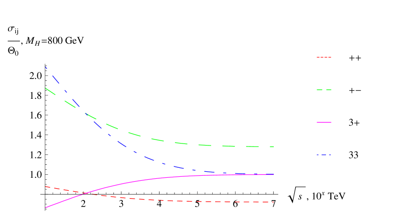
Figure 1: Case $\sqrt{s}\gg M_{H}>M_{W}$: ratio between the dressed cross sections and the invariant $\Theta_{0}$, as defined in (54), as function of the c.m. energy.

Figure 2: Left: Diagrammatic representation of the overlap matrix. The t-channel couples legs $1$ and $1^{\prime}$, while the choice of the momentum sign on the external legs fixes the conservation law for the generators of the considered symmetry as: $T_{1}^{a}-T_{1^{\prime}}^{a}=T_{2^{\prime}}^{a}-T_{2}^{a}$. Right: Feynman rules for the scalar-scalar-gauge interactions from (72) in the two situations $\omega>M_{H}$ and $\omega<M_{H}$. In the first case we have chosen the basis in which $\varphi_{4}\equiv h$. $T_{L}$ and $T_{V}$ are those defined in (74).

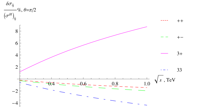
Figure 3: Case $\sqrt{s}\ll M_{H}$: ratio between the dressed cross sections and the tree level ones as function of the c.m. energy, at fixed scattering angle $\theta=\pi/2$ and for $M_{H}=800$ GeV.

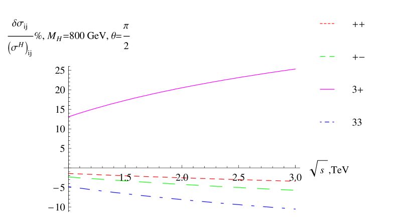
Figure 4: Case $\sqrt{s}\gg M_{H}>M_{W}$: ratio between the dressed cross sections and the tree level ones as function of the c.m. energy, at fixed scattering angle $\theta=\pi/2$ and for $M_{H}=800$ GeV.

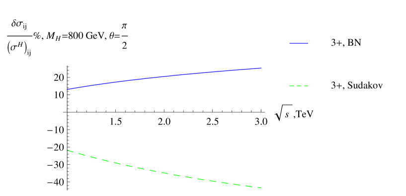
Figure 5: Case $\sqrt{s}\gg M_{H}>M_{W}$: Block-Nordsieck corrections vs. Sudakov corrections in the $\sigma_{3+}$ case. In the inclusive treatment the electroweak corrections change their sign compared to the exclusive case.

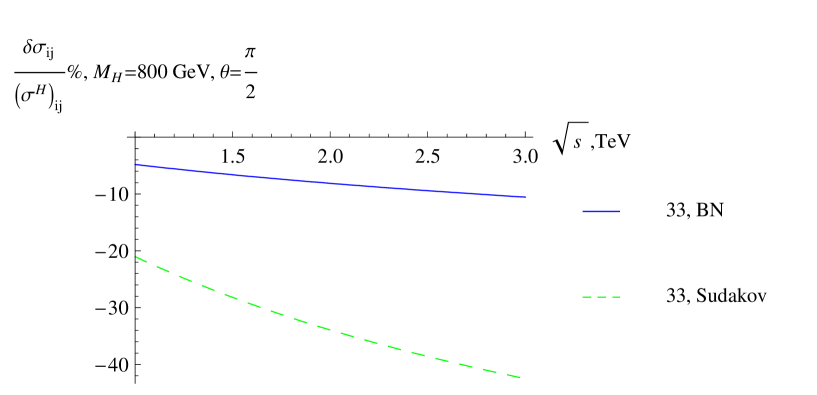
Figure 6: Case $\sqrt{s}\gg M_{H}>M_{W}$: Block-Nordsieck corrections vs. Sudakov corrections in the $\sigma_{33}$ case. In the inclusive treatment the electroweak corrections have the same sign if compared with the exclusive case, but the cross section results less suppressed.

Appendix A Appendix

In this appendix we illustrate the main symmetry proprieties of the Standard Model Lagrangian in the limit $g^{\prime}\rightarrow 0$, taking into account in particular the role of the gauge symmetry and of its global $SU(2)_{L}\otimes SU(2)_{R}$ extension.
Since we work considering just the scalar sector, our starting point is the Lagrangian of the $SU(2)$ gauged $\sigma$-model:

$$\mathcal{L}=-\frac{1}{2}Tr\left(\widehat{W}_{\mu\nu}\widehat{W}^{\mu\nu}\right)+\frac{1}{2}Tr\left[(D_{\mu}\Phi)^{{\dagger}}D^{\mu}\Phi\right]-\frac{\mu^{2}}{2}Tr\left(\Phi^{{\dagger}}\Phi\right)-\frac{\lambda}{4}\left[Tr\left(\Phi^{{\dagger}}\Phi\right)\right]^{2},$$ (62)

where the scalar content of the theory is organized into the following matrix:

$$\Phi\equiv\frac{1}{\sqrt{2}}\left(h\textbf{1}_{2\text{x}2}+i\varphi_{i}\tau_{i}\right)=\frac{1}{\sqrt{2}}\left(\begin{array}[]{cc}h+i\varphi_{3}&\varphi_{1}-i\varphi_{2}\\ \varphi_{1}+i\varphi_{2}&h-i\varphi_{3}\\ \end{array}\right)$$ (63)

and where, as usual:

$$\begin{array}[]{c}\widehat{W}_{\mu}\equiv\frac{1}{2}W_{\mu}^{k}\tau_{k},\\ \\ \widehat{W}_{\mu\nu}=\partial_{\mu}\widehat{W}_{\nu}-\partial_{\nu}\widehat{W}_{\mu}+ig\left[\widehat{W}_{\mu},\widehat{W}_{\nu}\right],\\ \\ D_{\mu}\Phi=\partial_{\mu}\Phi+ig\widehat{W}_{\mu}\Phi.\end{array}$$ (64)

Taking into account this notation, in which the matrix $\Phi$ acquires the standard “doublet-antidoublet” form, the gauge transformations, restricted to the isospin $SU(2)_{L}$ case in the limit $g^{\prime}\rightarrow 0$, are:

$$\begin{array}[]{c}ig\widehat{W}_{\mu}^{\prime}=g_{L}(x)ig\widehat{W}_{\mu}g_{L}^{{\dagger}}(x)+g_{L}(x)\partial_{\mu}g_{L}^{{\dagger}}(x),\\ \\ \widehat{W}_{\mu\nu}^{\prime}=g_{L}(x)\widehat{W}_{\mu\nu}g_{L}^{{\dagger}},\\ \\ \Phi^{\prime}=g_{L}(x)\Phi,\end{array}$$ (65)

where:

$$g_{L}(x)=\exp\left(i\alpha_{k}(x)\frac{\tau_{k}}{2}\right)\in SU(2)_{L}.$$ (66)

In order to clarify the transformation proprieties under the gauge symmetry, it’s straightforward to consider explicitly (65) for the scalar fields, obtaining:

$$\left\{\begin{array}[]{c}h\rightarrow h-\frac{1}{2}\varphi_{k}\delta_{kl}\alpha_{l}^{L}(x),\\ \\ \varphi_{k}\rightarrow\varphi_{k}+\frac{1}{2}h\alpha_{k}^{L}(x)+\frac{1}{2}\varepsilon_{klm}\varphi_{l}\alpha_{m}^{L}(x).\end{array}\right.$$ (67)

At this point it’s possible to see that the Lagrangian in (62), because of the limit $g^{\prime}\rightarrow 0$, has a larger global $SU(2)_{L}\otimes SU(2)_{R}$ symmetry, under which the scalar fields transform as:

$$\Phi^{\prime}=L\Phi R^{{\dagger}},$$ (68)

with $L\in SU(2)_{L}$ and $R\in SU(2)_{R}$ or, expanding the fields as in (63):

$$\left\{\begin{array}[]{c}h\rightarrow h+\frac{1}{2}\varphi_{k}\delta_{kl}\left(\alpha_{l}^{R}-\alpha_{l}^{L}\right)\\ \\ \varphi_{k}\rightarrow\varphi_{k}+\frac{1}{2}h\left(\alpha_{k}^{L}-\alpha_{k}^{R}\right)+\frac{1}{2}\varepsilon_{lmk}\varphi_{l}\left(\alpha_{m}^{R}+\alpha_{m}^{L}\right)\end{array}\right.$$ (69)

After electroweak symmetry breaking the global $SU(2)_{L}\otimes SU(2)_{R}$ symmetry is spontaneously broken into its diagonal custodial subgroup $SU(2)_{V}$; the transformation laws under this custodial symmetry for the scalar fields are:

$$\left\{\begin{array}[]{c}h\rightarrow h\\ \\ \varphi_{k}\rightarrow\varphi_{k}+\varepsilon_{lmk}\varphi_{l}\alpha_{m}=\varphi_{k}+i\left(T_{V}^{m}\right)_{kl}\alpha_{m}\varphi_{l}.\end{array}\right.$$ (70)

As a consequence the Higgs boson $h$ is a singlet, while the three Goldstone bosons are a triplet, transforming according to the adjoint representation of $SU(2)_{V}$.
Once assumed these transformation proprieties it’s possible to consider the explicit interactions in the Lagrangian (62) that we have used during our work.
Introducing the Higgs mass as function of the parameters in the scalar potential as $M_{H}^{2}=2\lambda v^{2}$, the interactions that involve the scalar fields are described by:

$$\mathcal{L}=-\frac{M_{H}^{2}}{8v^{2}}h^{4}-\frac{M_{H}^{2}}{2v}h^{3}-\frac{M_{H}^{2}}{4v^{2}}h^{2}\varphi_{k}\varphi_{l}\delta_{kl}-\frac{M_{H}^{2}}{2v}h\varphi_{k}\varphi_{l}\delta_{kl}-\frac{M_{H}^{2}}{8v^{2}}\left(\varphi_{k}\varphi_{l}\delta_{kl}\right)\left(\varphi_{m}\varphi_{n}\delta_{mn}\right),$$ (71)

while the gauge interactions of the scalar fields, written in the $g^{\prime}\rightarrow 0$ limit, are:

$$\mathcal{L}=\frac{g}{2}\delta_{kl}W_{\mu}^{l}\left[h\left(\partial^{\mu}\varphi_{k}\right)-\varphi_{k}\left(\partial^{\mu}h\right)\right]+\frac{g}{2}\varepsilon_{klm}\varphi_{k}W_{\mu}^{l}\left(\partial^{\mu}\varphi_{m}\right)+\frac{g^{2}v}{4}g^{\mu\nu}hW_{\mu}^{k}W_{\nu}^{l}\delta_{kl}.$$ (72)

Considering in particular the $3$-vertex interactions $\mathcal{L}(h\varphi W,\varphi\varphi W)$ of the previous Lagrangian, as in fig.2, it’s possible to construct the eikonal current that describes the emission of a soft gauge boson from a longitudinal one, with the possibility to have, as final state, a gauge boson as well as an Higgs boson, obtaining the current:

$$J^{\mu}(k,b;p)=\frac{gp^{\mu}}{2p\cdot k}\left[T^{b}_{V}\Theta_{W}+T^{b}_{H}\Theta_{H}\right]=\frac{gp^{\mu}}{p\cdot k}\left[T^{b}_{L}\Theta_{H}+\frac{1}{2}T^{b}_{V}\left(\Theta_{W}-\Theta_{H}\right)\right],$$ (73)

with:

$$\left(T^{b}_{L}\right)_{ac}=\frac{1}{2}\left(\begin{array}[]{cc}i\varepsilon_{abc}&-i\delta_{ab}\\ i\delta_{bc}&0\\ \end{array}\right)=\frac{1}{2}\left(T^{a}_{V}+T^{a}_{H}\right)\,\,\,\,\,\,\,\,\,\,\,\,\,\,\,\,\left(T^{b}_{R}\right)_{ac}\equiv\frac{1}{2}\left(\begin{array}[]{cc}i\varepsilon_{abc}&+i\delta_{ab}\\ -i\delta_{bc}&0\\ \end{array}\right)=\frac{1}{2}\left(T^{a}_{V}-T^{a}_{H}\right);$$ (74)

at this point the proprieties of symmetry follow directly from the commutation relations:

$$\left[T^{a}_{V},T^{b}_{V}\right]=i\varepsilon_{abc}T^{c}_{V}\,\,\,\,\,\,\,\,\,\,\,\left[T^{a}_{H},T^{b}_{H}\right]=i\varepsilon_{abc}T^{c}_{H}\,\,\,\,\,\,\,\,\,\,\,\left[T^{a}_{H},T^{b}_{H}\right]=i\varepsilon_{abc}T^{c}_{V},$$ (75)

and:

$$\left[T^{a}_{L},T^{b}_{L}\right]=i\varepsilon_{abc}T^{c}_{L}\,\,\,\,\,\,\,\,\,\,\,\left[T^{a}_{R},T^{b}_{R}\right]=i\varepsilon_{abc}T^{c}_{R}\,\,\,\,\,\,\,\,\,\,\,\left[T^{a}_{L},T^{b}_{R}\right]=0,$$ (76)

from which $\left\{T^{a=1,2,3}_{V},T^{a=1,2,3}_{H}\right\}$ are the six generators of the $O(4)$ group and $\left\{T^{a=1,2,3}_{L},T^{a=1,2,3}_{R}\right\}$ are the generators of the $SU(2)_{L}\otimes SU(2)_{R}\sim O(4)$ group; as a consequence, $\left\{T^{a=1,2,3}_{V}\right\}$ are the generators of the custodial $SU(2)_{V}$ diagonal subgroup.

References

• [1] C. Amsler et al., Physics Letters B667, 1 (2008). See also http://pdg.lbl.gov/
• [2] K. Agashe, S. Gopalakrishna, T. Han, G. Y. Huang and A. Soni, arXiv:0810.1497 [hep-ph]; K. Cheung, C. W. Chiang and T. C. Yuan, Phys. Rev.  D 78 (2008) 051701; B. Bellazzini, S. Pokorski, V. S. Rychkov and A. Varagnolo, JHEP 0811 (2008) 027 [arXiv:0805.2107 [hep-ph]]; G. F. Giudice, C. Grojean, A. Pomarol and R. Rattazzi, JHEP 0706 (2007) 045. See also G. F. Giudice, J. Phys. Conf. Ser. 110 (2008) 012014 and references therein.
• [3] C. Englert, B. Jager, M. Worek and D. Zeppenfeld, arXiv:0810.4861 [hep-ph]; A. Ballestrero, G. Bevilacqua and E. Maina, arXiv:0812.5084 [hep-ph]; J. M. Butterworth, B. E. Cox and J. R. Forshaw, Phys. Rev.  D 65 (2002) 096014; J. Bagger et al., Phys. Rev.  D 52 (1995) 3878.
• [4] E. Accomando, A. Denner and S. Pozzorini, JHEP 0703 (2007) 078.
• [5] P.Ciafaloni and A. Urbano, in preparation
• [6] M. Kuroda, G. Moultaka and D. Schildknecht, Nucl. Phys. B 350 (1991) 25; G. Degrassi and A. Sirlin, Phys. Rev. D 46, 3104 (1992); A. Denner, S. Dittmaier and R. Schuster, Nucl. Phys. B 452, 80 (1995); A. Denner, S. Dittmaier and T. Hahn, Phys. Rev. D 56, 117 (1997); A. Denner and T. Hahn, Nucl. Phys. B 525, 27 (1998); W. Beenakker, A. Denner, S. Dittmaier, R. Mertig and T. Sack, Nucl. Phys. B 410, 245 (1993); W. Beenakker, A. Denner, S. Dittmaier and R. Mertig, Phys. Lett. B 317, 622 (1993). M. Beccaria, G. Montagna, F. Piccinini, F. M. Renard and C. Verzegnassi, Phys. Rev. D 58 (1998) 093014. P. Ciafaloni and D. Comelli, Phys. Lett. B 446, 278 (1999); V. S. Fadin, L. N. Lipatov, A. D. Martin and M. Melles, Phys. Rev. D 61 (2000) 094002; P. Ciafaloni, D. Comelli, Phys. Lett. B 476 (2000) 49; J. H. Kuhn, A. A. Penin and V. A. Smirnov, Eur. Phys. J. C 17, 97 (2000); J. H. Kuhn, S. Moch, A. A. Penin, V. A. Smirnov, Nucl. Phys. B 616, 286 (2001) [Erratum-ibid. B 648, 455 (2003)]; M. Melles, Phys. Rept. 375, 219 (2003); J. y. Chiu, F. Golf, R. Kelley and A. V. Manohar, Phys. Rev.  D 77 (2008) 053004; J. y. Chiu, R. Kelley and A. V. Manohar, Phys. Rev.  D 78 (2008) 073006.
• [7] M. Ciafaloni, P. Ciafaloni and D. Comelli, Phys. Rev. Lett. 84, 4810 (2000); Phys. Lett. B 501, 216 (2001); Nucl.Phys. B 589 359 (2000); Phys. Rev. Lett. 88, 102001 (2002); Phys. Rev. Lett. 87 (2001) 211802; JHEP 0805 (2008) 039; P. Ciafaloni, D. Comelli and A. Vergine, JHEP 0407, 039 (2004); M. Ciafaloni, Lect. Notes Phys.  737 (2008) 151; M. Ciafaloni, P. Ciafaloni and D. Comelli, Phys. Lett. B 501, 216 (2001); P. Ciafaloni and D. Comelli, JHEP 0609, 055 (2006); JHEP 0511 (2005) 022.
• [8] M. Ciafaloni, P. Ciafaloni and D. Comelli, Nucl. Phys.  B 613, 382 (2001).
• [9] U. Baur, Phys. Rev. D 75 (2007) 013005; R. S. Thorne, arXiv:0711.2986 [hep-ph].
• [10] G. Bozzi, B. Jager, C. Oleari and D. Zeppenfeld, Phys. Rev.  D 75 (2007) 073004; B. Jager, C. Oleari and D. Zeppenfeld, Phys. Rev.  D 73 (2006) 113006; B. Jager, C. Oleari and D. Zeppenfeld, JHEP 0607 (2006) 015