Electromagnetic Pulse Driven Spin-dependent Currents in Semiconductor Quantum Rings

Abstract

We investigate the non-equilibrium charge and spin-dependent currents in a quantum ring with a Rashba spin orbit interaction (SOI) driven by two asymmetric picosecond electromagnetic pulses. The equilibrium persistent charge and persistent spin-dependent currents are investigated as well. It is shown that the dynamical charge and the dynamical spin-dependent currents vary smoothly with a static external magnetic flux and the SOI provides a SU(2) effective flux that changes the phases of the dynamic charge and the dynamic spin-dependent currents. The period of the oscillation of the total charge current with the delay time between the pulses is larger in a quantum ring with a larger radius. The parameters of the pulse fields control to a certain extent the total charge and the total spin-dependent currents. The calculations are applicable to nano-meter rings fabricated in heterojuctions of III-V and II-VI semiconductors containing several hundreds electrons.

I Introduction

Study of the spin-orbit interaction (SOI) in semiconductor low dimensional structures and its application for spintronics devices have attracted much attention recently spintronics . There are two important kinds of SOI in conventional semiconductors: one is the Dresselhaus SOI induced by bulk inversion asymmetry dresselhaus , and the other is the Rashba SOI caused by structure inversion asymmetry rashba . As pointed out in lommer , the Rashba SOI is dominant in a narrow gap semiconductor system and the strength of the Rashba SOI can be tuned by an external gate voltage in HgTe hgte , InAs luo , In_xGa_1-xAs nitta , and GaAs rashba ; malcher quantum wells. Recent research is focused on the electrically-induced generation of a spin-dependent current (SC) mediated by SOI-type mechanism, e.g. as in the intrinsic spin Hall effect in a 3D p-doped semiconductor murakami and in a 2D electron gas with Rashba SOI sinova . Here we study a high quality spin-interacting quantum rings (QRs) with a radius on the nanometer scale fuhrer ; ring . These systems show Aharonov-Bohm-type (AB) spin-interferences nitta99 ; nitta03 . In particular we investigate the dynamics triggered by time-dependent electric fields as provided by time-asymmetric pulses hcp or tailored laser pulse sequences bennett . The quantity under study is the spin-resolved pulse-driven current, in analogy to the spin-independent case matos05 ; pershin ; rasanen . In a previous work zhu , we investigated the dynamical response of the charge polarization to the pulse application. No net charge or spin-dependent current is generated because the clock-wise and anti-clock-wise symmetry of the carrier is not broken by one pulse or a series of pulses having the same linear polarization axis. This symmetry is lifted if two time-delayed pulses with non-collinear polarization axes are applied matos05 . However, to our knowledge all previous studies on light-induced currents in quantum rings did not consider the coupling of the spin to the orbital motion (and hence to the light field), which is addressed in this work. As detailed below, having done that, it is possible to control dynamically the spin-dependent current in a 1D quantum ring with Rashba SOI by using two time-delayed linearly polarized electromagnetic pulses. For transparent interpretation of the results only the Rashba SOI is considered in this work. The presence of the Dresselhaus SOI may change qualitatively the results presented here for the spin-dependent non-equilibrium dynamic of the carriers, which can be anticipated from the findings on for the equilibrium case ref1 .

II Theoretical model

We study the response of charges and spins confined in a one-dimensional (1D) ballistic QR with SOI to the application of two short time-delayed linearly polarized asymmetric electromagnetic pulses matos05 ; matos . The effective single particle Hamiltonian reads $\hat{H}^{\prime}=\hat{H}_{\mbox{SOI}}+\hat{H}_{1}(t)$ zhu , with

$$\hat{H}_{\mbox{SOI}} = \frac{\mathbf{p}^{2}}{2m^{*}}+V(\mathbf{r})+\frac{\alpha_{R}}{\hbar}(\hat{\mathbf{\sigma}}\times\mathbf{p})_{z},\hat{H}_{1}(t)=-e\mathbf{r}\cdot\mathbf{E}(t)+\mu_{B}\mathbf{B}(t)\cdot\hat{\mathbf{\sigma}}.$$ (1)

$\mathbf{E}(t)$ and $\mathbf{B}(t)$ are the electric and the magnetic fields of the pulse. Integrating out the $r$ dependence $\hat{H}_{\mbox{SOI}}$ reads in cylindrical coordinates meijer ; frustaglia ; molnar ; foldi ; sheng

$$\hat{H}_{\mbox{SOI}}=\frac{\hbar\omega_{0}}{2}[(i\partial_{\varphi}+\frac{\phi}{\phi_{0}}-\frac{\omega_{R}}{2\omega_{0}}\sigma_{r})^{2}-(\frac{\omega_{R}}{2\omega_{0}})^{2}+\frac{\omega_{B}}{\omega_{0}}\sigma_{z}].$$ (2)

$\partial_{\varphi}=\frac{\partial}{\partial\varphi}$, $\phi_{0}=h/e$ is the flux unit, $\phi=B\pi a^{2}$ is the magnetic flux threading the ring, $a$ is the radius of the ring, $\hbar\omega_{0}=\hbar^{2}/(m^{*}a^{2})=2E_{0}$, $\hbar\omega_{R}=2\alpha_{R}/a$, $\hbar\omega_{B}=2\mu_{B}B$ and $B$ are due to a possible external static magnetic field $\mathbf{B}=B\hat{\mathbf{e}}_{z}$. The single-particle eigenstates of $\hat{H}_{\mbox{SOI}}$ are represented as $\Psi_{n}^{S}(\varphi)=e^{i(n+1/2)\varphi}\nu^{S}(\gamma,\varphi)$ where $\nu^{S}(\gamma,\varphi)=(a^{S}e^{-i\varphi/2},b^{S}e^{i\varphi/2})^{T}$ are spinors in the angle dependent local frame, and $a^{\uparrow}=\cos(\gamma/2),\;b^{\uparrow}=\sin(\gamma/2),\;a^{\downarrow}=-\sin(\gamma/2),b^{\downarrow}=\cos(\gamma/2),$ (T means transposed) where $\tan\gamma=-Q_{R}=-\omega_{R}/\omega_{0}$ (if we ignore the Zeeman splitting caused by the static magnetic field sheng ; splett ). $\gamma$ describes the direction of the spin quantization axis, as illustrated in Fig. (1a). The energy spectrum of the QR with the SOI reads frustaglia ; molnar ; foldi ; sheng ; splett ; zhu

$$E_{n}^{S}=\frac{\hbar\omega_{0}}{2}\left[(n-\phi/\phi_{0}+\frac{1-Sw}{2})^{2}-\frac{Q_{R}^{2}}{4}\right],$$ (3)

$$w=\sqrt{1+Q_{R}^{2}}=1/\cos\gamma,$$

where $S=+1\,(S=-1)$ stands for spin up (spin down) in the local frame.

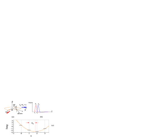
Figure 1: (Color online) (a) Schematic graph of the geometry, spin configuration and the applied pulses is shown. (b) Time-delayed asymmetric pulses are schematically drawn. (c) Energy spectrum for a ring with spin orbit interaction. $\Delta_{S}$ defines the distance between the spectrum symmetry axis and the smallest nearest integer.

III Pulse-driven single-particle dynamics

We apply two time-asymmetric pulses to the system (see Fig. (1b)). The first one (at $t=0$) propagates in the $z$ direction and has a duration $\tau_{d}$. Its E-field is along the $x$ direction. $\tau_{d}$ is chosen much shorter than the ballistic time of the carriers in which case the QR states develop as matos05 ; matos ; mizushima

$$\Psi_{n}^{S}(\varphi,t>0)=\Psi_{n}^{S}(\varphi,t<0)e^{i\alpha_{1}\cos\varphi},\;\alpha_{1}=eap/\hbar,\;p=-\int_{0}^{\tau_{d}}E(t)dt,$$ (4)

where $E(t)=Ff(t)$, $F$ and $f(t)$ describe the amplitude and the time dependence of the electric field of the pulse respectively. In the following, we use $F_{1}$ and $F_{2}$ to characterize the first and the second pulses. The pulse effect is encapsulated entirely in the action parameter $\alpha_{1}$. With the initial conditions $n(t<0)=n_{0}$ and $S(t<0)=S_{0}$ and using Eq. (4) one finds

$$\Psi_{n_{0}}^{S_{0}}(\varphi,t)=\frac{1}{\sqrt{2\pi}}\sum_{ns}C_{n}^{S}(n_{0},S_{0},t)e^{i(n+1/2)\varphi}e^{-iE_{n}^{S}t/\hbar}|\nu^{S}\rangle,$$ (5)

with

$$C_{n}^{S}=\left\{\begin{array}[]{l l}\delta_{SS_{0}}\delta_{nn_{0}}&\mbox{for t}\leq 0,\\ \delta_{SS_{0}}i^{n_{0}-n}J_{n_{0}-n}(\alpha_{1})&\mbox{for t}>0,\end{array}\right.$$ (6)

where $J_{n}$ is the n-th order Bessel function. For the time-dependent energy we find

$$E_{n_{0}}^{S_{0}}(t>0)=E_{n_{0}}^{S_{0}}(t<0)+\frac{\hbar\omega_{0}}{2}\frac{\alpha^{2}_{1}}{2},$$ (7)

with $E_{n_{0}}^{S_{0}}(t<0)$ is given by Eq. (3). Applying a second pulse at $t=\tau$ with the same duration $\tau_{d}$ but the electric field being along the $y$ axis (see Fig. (1b)), the wave functions develop as $\Psi_{n_{0}}^{S_{0}}(\varphi,t>\tau)=\Psi_{n_{0}}^{S_{0}}(\varphi,t<\tau)e^{i\alpha_{2}\sin\varphi}$, where $\alpha_{2}$ is the action parameter associated with the second pulse. $\Psi_{n_{0}}^{S_{0}}(\varphi,t=\tau^{-})$ follows from Eq. (5). For $t>\tau$ the expansion coefficients behave as $C_{n^{\prime}}^{S^{\prime}}(n_{0},S_{0},t>\tau)=\sum_{n}\delta_{S^{\prime}S_{0}}[i^{n_{0}-n}J_{n_{0}-n}(\alpha_{1})\;J_{n^{\prime}-n}(\alpha_{2})]e^{i(E_{n^{\prime}}^{S^{\prime}}-E_{n}^{S_{0}})\tau/\hbar}.$

IV Nonequilibrium spin and charge currents

A single pulse does not generate in QR any net charge current because of the degeneracy of the orbital states. However, the charge will be polarized matos ; zhu and corresponding dipole moments oscillate in the $x$ direction with an associated optical emission. Applying a second pulse as described above leads to a non-equilibrium net current, in addition to the persistent charge current caused by the static flux and the SOI which causes a SU(2) vector potential and manifests itself in an induced spin-dependent persistent charge current sheng ; splett ; oh ; frohlich . Consequently, a non-equilibrium spin-dependent current is induced.

The line velocity operator is ballentine

$$\hat{\mathbf{v}}_{\varphi}=\hat{\mathbf{e}}_{\varphi}\left\{\frac{-i\hbar}{m^{*}a}\partial_{\varphi}-\frac{\hbar}{m^{*}a}\frac{\phi}{\phi_{0}}+\frac{\alpha_{R}}{\hbar}\sigma_{r}\right\}$$

which is associated to the operator of the angular velocity $\hat{\mathbf{v}_{\varphi}}/a$ loss . Contributions to the persistent charge current from each QR level read wendler

$$\mathbf{I}_{n_{0},S_{0}}=\frac{1}{2\pi}\int_{0}^{2\pi}d\varphi\int_{r_{1}}^{r_{2}}dr\mathbf{j}^{\varphi}_{n_{0},S_{0}}(\mathbf{r}^{\prime},t>\tau),$$

where

$$\mathbf{j}^{\varphi}_{n_{0},S_{0}}=e\Re[\Psi_{n_{0}}^{S_{0},{\dagger}}(\mathbf{r}^{\prime},t)\hat{\mathbf{v}}_{\varphi}\Psi_{n_{0}}^{S_{0}}(\mathbf{r}^{\prime},t)].$$

Upon algebraic manipulations we find

$$\mathbf{I}_{n_{0},S_{0}}(t>\tau)=\mathbf{I}_{n_{0},S_{0}}^{(0)}(t>\tau)+\mathbf{I}_{n_{0},S_{0}}^{(1)}(t>\tau).$$ (8)

The index “(0)” stands for the static persistent charge current (PCC) which exists in the absence of pulse field, whereas the index “(1)” indicates the pulse-induced dynamic charge current (DCC). The PCC is caused by a magnetic U(1) flux and has been studied extensively pccreview without wendler ; buttiker ; chakraborty or with the spin interactions loss . It has been experimentally observed both in gold rings of radius with 1.2 and 2.0 $\mu$m chandrasekhar and in a GaAs-AlGaAs ring of radius about 1 $\mu$m mailly . The SOI scattering effects were also studied sopcc . The PCC carried by the states characterized by $n_{0}$ and $S_{0}$ reads (please note the current in this work is defined as flow of positive charges, which is opposite to the direction of flow of electrons)

$$\mathbf{I}_{n_{0},S_{0}}^{(0)}(t>\tau)=\hat{\mathbf{e}}_{\varphi}I_{0}\left(n_{0}-\frac{\phi}{\phi_{0}}+\frac{1-S_{0}w}{2}\right),$$ (9)

where $I_{0}=2E_{0}a/\phi_{0}$ is the unit of CC, the second term on the right hand side of Eq. (9) stems from the static magnetic field; the third term is a consequence of the SU(2) flux of the SOI sheng . The DCC part is

$$\mathbf{I}_{n_{0},S_{0}}^{(1)}(t>\tau)=\hat{\mathbf{e}}_{\varphi}I_{0}\left\{\alpha_{2}\langle\cos\varphi\rangle_{n_{0}}^{S_{0}}(\tau)\right\},$$ (10)

where

$$\langle\cos\varphi\rangle_{n_{0}}^{S_{0}}(\tau)=\alpha_{1}h(\Omega_{\tau 1})\sin b_{\tau}\cos[2(n_{0}-\frac{\phi}{\phi_{0}}+\frac{1-S_{0}w}{2})b_{\tau}],$$

$$b_{\tau}=\omega_{0}\tau/2,$$

$$\Omega_{\tau 1}=\alpha_{1}\sqrt{2(1-\cos(2b_{\tau}))},$$

$$h(\Omega_{\tau 1})=J_{0}(\Omega_{\tau 1})+J_{2}(\Omega_{\tau 1}).$$

To obtain the total persistent charge current and the dynamic current we have to consider the spin-resolved occupations of the single particle states. For simplicity we operate at zero temperatures and ignore the relaxation caused by phonons or other mechanisms, i.e. we confine ourself to times shorter than the relaxation time. The general case can be developed along the line of Ref. moskalenko .

At first we introduce an effective flux as

$$\phi_{S}=\phi-\phi_{0}\frac{1-Sw}{2}.$$ (11)

As evident from Eq. (3) the spectrum is symmetric with respect to $x_{S}=\phi_{S}/\phi_{0}$. Further we define the shift $\Delta_{S}=x_{S}-l(l^{\prime})$, where $S=\uparrow$ or $\downarrow$. Here $l(l^{\prime})=[x_{\uparrow(\downarrow)}]$ where $[x]$ means the nearest integer which is less than $x$. $\Delta_{S}$ is shown in Fig. 1. When $\Delta_{S}=1$, it is equivalent to $\Delta_{S}=0$. Furthermore, $\bar{\Delta}_{S}=|1/2-\Delta_{S}|$ is the distance between the $x_{S}$ and the nearest half integer.

IV.1 Spinless Particles

For $N$ spinless particles we distinguish two cases: N is an even or an odd integer.

Case (1): If N is an even integer then

$$I_{\mbox{even}}^{(0)}(\Delta) = \mbox{sgn}(\Delta)N(\frac{1}{2}-\Delta),\>$$ (12)

$$I_{\mbox{even}}^{(1)}(\Delta) = \alpha_{1}\alpha_{2}h(\Omega_{\tau_{1}})\sin(Nb_{\tau})\cos(1-2\Delta)b_{\tau},$$ (13)

where $\mbox{sgn}(x)$ equals +1, for $x>0$; 0 for $x=0$, and -1 for $x<0$. Case (2): If N is an odd integer then

$$I_{\mbox{odd}}^{(0)}(\Delta) = -\mbox{sgn}(\Delta)\mbox{sgn}(\frac{1}{2}-\Delta)N(\frac{1}{2}-\bar{\Delta}),\>$$ (14)

$$I_{\mbox{odd}}^{(1)}(\Delta) = \alpha_{1}\alpha_{2}h(\Omega_{\tau_{1}})\sin(Nb_{\tau})\cos(1-2\bar{\Delta})b_{\tau}.$$ (15)

IV.2 Particles with 1/2 spin

For spin 1/2 particles we consider four cases.

Case (0): For an even number of particles’ pairs, i.e. $N=4m$, where $m$ is an integer we find

$$I_{S}^{(0)}(\Delta_{S})=I_{\mbox{even}}^{(0)}(\Delta_{S}),\,I_{S}^{(1)}(\Delta_{S})=I_{\mbox{even}}^{(1)}(\Delta_{S}),$$ (16)

Case (1): For an odd number of particles’ pairs, i.e. $N=4m+2$ we obtain

$$I_{S}^{(0)}(\Delta_{S})=I_{\mbox{odd}}^{(0)}(\Delta_{S}),I_{S}^{(1)}(\Delta_{S})=I_{\mbox{odd}}^{(1)}(\Delta_{S}).$$ (17)

Case (2): For an even number of pairs plus one extra particle, i.e. $N=4m+1$ (there is one particle whose spin is unpaired as compared with case (0)) we find

$$I_{\mbox{ext},S}^{(0)}(\Delta_{S}) = -\mbox{sgn}(\Delta_{S})\mbox{sgn}(\frac{1}{2}-\Delta_{S})(\frac{N-1}{4}+\frac{1}{2}-\bar{\Delta}_{S}),\>$$ (18)

$$I_{\mbox{ext},S}^{(1)}(\Delta_{S}) = \alpha_{1}\alpha_{2}h(\Omega_{\tau_{1}})\sin(b_{\tau})\cos(\frac{N-1}{2}+1-2\bar{\Delta}_{S})b_{\tau}.$$ (19)

To determine which spin state is occupied by the extra particle one compares the distance of the symmetric axis to the nearest half integral axis, i.e. $\bar{\Delta}_{S}$. The one with the larger distance will be occupied.

Case (3): For an odd number of pairs plus one extra particle, i.e. $N=4m+3$. Here we use case (1) and determine the contribution to the current from the extra particle

$$I_{\mbox{ext,S}}^{(0)}(\Delta_{S}) = \mbox{sgn}(\Delta_{S})\mbox{sgn}(\frac{1}{2}-\Delta_{S})(\frac{N-3}{4}+\frac{1}{2}+\bar{\Delta}_{S}),\>$$ (20)

$$I_{\mbox{ext,S}}^{(1)}(\Delta_{S}) = \alpha_{1}\alpha_{2}h(\Omega_{\tau_{1}})\sin(b_{\tau})\cos(\frac{N-3}{2}+1+2\bar{\Delta}_{S})b_{\tau}.$$ (21)

Which spin state is occupied by the extra particle is governed by $\bar{\Delta}_{S}$. The level with the smaller $\bar{\Delta}_{S}$ is populated.

V spin-dependent current (SC)

In presence of a static magnetic field and the SOI but in the absence of the pulse field the PCC is accompanied with a persistent SC (PSC). Switching on the pulse field generates a spin-dependent charge currents due to the SOI, and also a dynamic SC (DSC) that can be controlled by the parameters of the pulse field. The SC density is

$$\mathbf{j}_{n_{0},S_{0}}^{s}(\mathbf{r}^{\prime},t)=\Re\{\Psi_{n_{0}}^{S_{0},{\dagger}}(\mathbf{r}^{\prime},t)\hat{\mathbf{v}}^{\prime}\hat{\mathbf{s}}\Psi_{n_{0}}^{S_{0}}(\mathbf{r}^{\prime},t)\},$$

where

$$\hat{\mathbf{s}}=(\hbar/2)\hat{\sigma_{z}}\delta(\mathbf{r}^{\prime}-\mathbf{r})$$

is the local spin density. The SC associated with level $n_{0},S_{0}$ is

$$\mathbf{I}_{n_{0},S_{0}}^{s}(t>\tau)=\frac{1}{2\pi}\int_{0}^{2\pi}d\varphi\int_{r_{1}}^{r_{2}}dr^{\prime}\mathbf{j}_{n_{0},S_{0}}^{s}(\mathbf{r}^{\prime},t)$$ (22)

and can be evaluated as

$$\mathbf{I}_{n_{0},S_{0}}^{s_{z}}=\mathbf{I}_{s0}\Re\sum_{n}|C_{n}^{S_{0}}(n_{0},S_{0},t)|^{2}D_{1n}^{S_{0}},$$ (23)

where

$$\mathbf{I}_{s0}=\hat{\mathbf{e}}_{\varphi}E_{0}a/(2\pi)$$

sets the unit SC and

$$D_{1n}^{S_{0}}=[(a^{S_{0}})^{2}-(b^{S_{0}})^{2}](n-\frac{\phi}{\phi_{0}})-(b^{S_{0}})^{2}.$$ (24)

Here

$$(a^{S_{0}})^{2}-(b^{S_{0}})^{2}=S_{0}\cos\gamma,$$

and $S_{0}=\pm 1$. The SC after applying two pulses to the ring is a sum of two parts

$$\mathbf{I}_{n_{0},S_{0}}^{s_{z}}(t>\tau)=\mathbf{I}_{n_{0},S_{0}}^{s_{z},(0)}(t>\tau)+\mathbf{I}_{n_{0},S_{0}}^{s_{z},(1)}(t>\tau),$$ (25)

where

$$\mathbf{I}_{n_{0},S_{0}}^{s_{z},(0)}(t>\tau) = \mathbf{I}_{s0}[S_{0}\cos\gamma][(n-\frac{\phi}{\phi_{0}})+\frac{1}{2}-\frac{S_{0}}{2\cos\gamma}],\>$$ (26)

$$= \mathbf{I}_{s0}[S_{0}\cos\gamma]\frac{I_{n_{0},S_{0}}^{(0)}(t>\tau)}{I_{0}},$$ (27)

is the static PSC sheng and the DSC part is

$$\mathbf{I}_{n_{0},S_{0}}^{s_{z},(1)}(t>\tau) = \mathbf{I}_{s0}[S_{0}\cos\gamma][\alpha_{2}\langle\cos\varphi\rangle_{n_{0},S_{0}}(\tau)],\>$$ (28)

$$= \mathbf{I}_{s0}[S_{0}\cos\gamma]\frac{I_{n_{0},S_{0}}^{(1)}(t>\tau)}{I_{0}}.$$ (29)

Summing over all occupied energy levels we find

$$\mathbf{I}_{S_{0}}^{s_{z}}(t>\tau)=\mathbf{I}_{S_{0}}^{s_{z},(0)}(t>\tau)+\mathbf{I}_{S_{0}}^{s_{z},(1)}(t>\tau),$$ (30)

where ($I_{S_{0}}^{(0),(1)}(t>\tau)$ are PCC and DCC)

$$\mathbf{I}_{S_{0}}^{s_{z},(0),(1)}(t>\tau)=\mathbf{I}_{s0}[S_{0}\cos\gamma]\frac{I_{S_{0}}^{(0),(1)}(t>\tau)}{I_{0}}.$$ (31)

VI Numerical Results and Discussions

We performed calculations for pulse-driven ballistic quantum rings fabricated by an appropriate confinement in a quantum well of In_xGa_1-xAs/InP thsch . Our results are also valid for other III-V or II-VI semiconductor quantum rings with spin orbit, e.g. GaAs-AlGaAs quantum well, or HgTe/HgCdTe quantum ring konig . We shall present the total charge current (TCC) which is a sum of PCC and DCC over all the occupied states. Total spin-dependent current (TSC) is obtained in the same way splett .

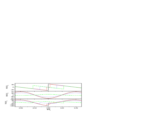
Figure 2: (Color online) Persistent charge current (PCC), dynamic charge current (DCC) and total charge current (TCC) are shown in (a), (b) and (c) respectively. The spin orbit angle are $\gamma=0^{\circ},-20^{\circ},-40^{\circ}$ and $-50^{\circ}$ for the solid lines, the dash lines, the dot lines and the dash-dot lines respectively in all graphs. The other parameters are $N=100$, $a=100$ nm, $\tau=26.3$ ps, $F_{1}=F_{2}=1$ kV/cm.

Fig. 2 shows how the flux and the SOI affect the PCC, DCC and TCC. Without the SOI, the jump of the PCC occurs at integer flux for even pair occupation, shown in Fig. 2. The jumps are different in other occupations (see splett ), here we only focus on the even pair occupation case for clarity. The periodic sawtooth dependence of the PCC on the flux exhibits has been studied before, e.g. sheng ; splett . At finite SOI the jumps in PCC are shifted to $\phi/\phi_{0}=l+(1\mp w)/2$; the two jumps are the consequences of a superposition of the contributions from the two spin channels. When the SOI strength is such that $\gamma=-\arccos(1/2n)$, ($n=1,2,\cdots$) the two jumps become at the half integer which is just the case of $4n+2$ occupation in absence of the SOI splett . The slope ratio between the two jumps is the same. As can be inferred from the analytic expressions DCC (cf. Fig. 2) depends smoothly on the flux. SOI results in a phase shift moving or even exchanging the positions of the minima and maxima, as is for $\gamma=-60^{\circ}$. The origin of the shape of TCC is deduced from those of PCC and DCC. Here the magnitudes of the two contributions is crucial: The PCC magnitude is related to the numbers of charge carriers, while the DCC magnitude is determined primarily by the product of the $\alpha_{1}$ and $\alpha_{2}$ (that can be externally varied by changing the pulse intensities), the delay time $\tau$, and the ring radius.

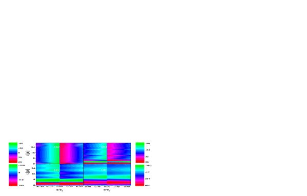
Figure 3: (Color online) Contour plots of TCC on $\phi$ and $\tau$ are shown for different radius of the ring. $a=100$ nm, 200 nm, 300 nm and 400 nm in (a), (b), (c) and (d) respectively. The other parameters are $N=100$, $\gamma=0^{\circ}$, $F_{1}=F_{2}=500$ V/cm.

Fig. 3 shows the TCC dependence on the ring radius (in the absence of the SOI). As expected, a larger $\alpha$ enhances the DCC. On the other hand, $\alpha$ enters the Bessel function argument whose increase suppresses the magnitude of DCC. It can be shown that the period of the oscillation with $\tau$ increases with increasing the radius. The magnitudes of the maxima and minima are larger with larger radius.

Now we discuss the spin-dependent current projected onto the $z$ direction sheng , i.e. $I^{S_{z}}$. The spin-dependent current projected onto the $\gamma$ direction (e.g. the quantization axis of the local spin frame) is $I^{S_{z}}=I^{\gamma}\cos\gamma$ splett .

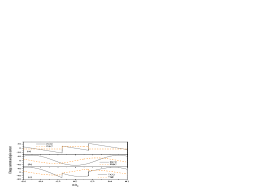
Figure 4: (Color online) PCC and PSC, DCC and DSC, and TCC and TSC are shown in (a), (b) and (c) respectively. The solid lines are the charge current, and the dash lines are the spin current. $\gamma=-40^{\circ}$, the other parameters are the same to Fig. 2.

PSC posses steps at PCC jumps (Fig. 4(a)) as a function of $\phi$. This can be understood from the ratio of PCC for different spins; the SOI only introduces a relative effective flux shift (see Eq. (11)) leading to a constant spin-dependent current between the jumps. For DSC vs. $\phi$ (Fig. 4(b)) the effective flux leads to a shift of the DSC along the flux axis. The physics behind this shift is that SOI provides a SU(2) flux, meaning that the pulse-driven (local frame) spin-up electrons experience a different flux than those with down spin, leading to a substantial spin-dependent current. In contrast, a static magnetic flux does not induce a spin-dependent current in the absence of the SOI. This shift and the jumps in the step function of the PSC explain the behaviour of TCC in Fig. 4(c).

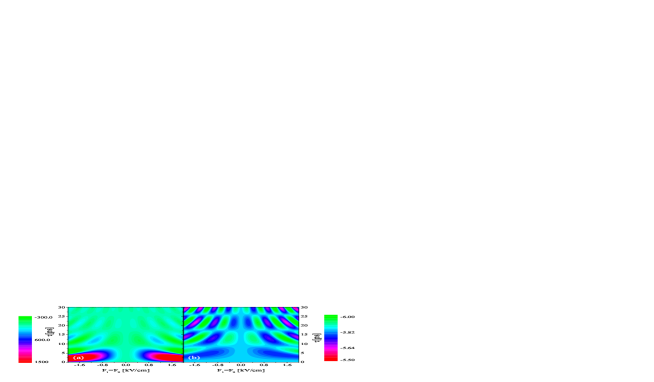
Figure 5: (Color online) TCC (a) and TSC (b) vs. pulses strengths $F_{1}=F_{2}$ and delay time $\tau$. $\gamma=-40^{\circ}$, $\phi=0.2$. Other parameters are $N=100$, $a=400$ nm.

The control of TCC and TSC by tuning the pulse-field parameters is demonstrated in Fig. 5. Because the two pulses transfer a net angular momentum setting the electrons in motion but they do not couple directly to the spins the TCC and TSC show the same pattern with $\tau$ and $F$. From an experimental point of view it is essential to note that we are dealing with non-equilibrium quantities which opens the way for their detection via their emission. E.g., the TCC and TSC can be detected by measuring the current-induced magnetization of the ring and the generated electrostatic potential scm .

VII General and concluding remarks

In presence of spin-orbit coupling, two time-delayed appropriately shaped electromagnetic pulses generate spin-dependent charge currents. As shown previously for the spin-independent case matos05 , the sign of the current and its magnitude are controllable via the delay time and the strengths of the pulses. From a symmetry viewpoint, similar phenomena may be expected to occur for other geometries (wires, squares, etc). However, as shown for unbiased superlattices moskalenko1 (without SOI) details of the generated currents may differ qualitatively. Application of an appropriate train of pulses open the possibility of controlling or even stopping the current moskalenko . For increasing the magnitude of the current more intense pulses should be applied.

For generating currents in quantum rings one may also apply circular polarized laser pulses pershin ; rasanen . In this context we note the following: From an electrodynamics point of view, generating currents by our pulses is a completely classical effect, i.e. currents are generated in a completely classical system, even though in our case the subsequent excited carrier evolution is quantum mechanical. For this reason our current is robust to disorder and geometry modifications. In addition, the tunable time delay between the pulses allows an ultra-fast control the current properties. Using circular polarized laser pulses generates currents for quantized systems (in which case the rotating-wave approximation can be applied). For systems with level broadening on the order of level spacing no appreciable current is generated. Our disadvantage however is that our pulses are much more demanding to realize experimentally, whereas laser pulses are readily available, in particular at high light intensities allowing thus for a strong current generation.

The DSC is proportional to the DCC which can be comparable to the PCC for small or moderate occupation number case as seen in Fig. (4b). The DCC depends on the strength of the field and the delayed time between the two pulses sensitively and dramatically. We provide now an explicit calculation for the typical values of the CC and SC. For In_xGa_1-xAs /InP quantum well thsch we have $m^{*}=0.037m_{0}$. For a ring with radius of 100 nm, the line velocity is then about $5000m/s$, and the current unit is $I_{0}/a\sim 8nA$ which corresponds to the angular velocity current for one particle. If we convert it into the unit of an induced magnetization it is a radius-independent quantity $M_{0}\approx$2 meV/T (here we use the formula $M_{0}\approx\pi a^{2}(I_{0}/a)$ valid for rings considered here matos05 ).

The work is support by the cluster of excellence ”Nanostructured Materials” of the state Saxony-Anhalt.

References

- (1) For a review on spintronics, see, e.g., S. A. Wolf, et al., Science 294, 1488 (2001).
- (2) G. Dresselhaus, Phys. Rev. 100, 580 (1955).
- (3) E. I. Rashba, Sov. Phys. Solid State 2, 1109 (1960); Y. A. Bychkov, and E. I. Rashba, J. Phys. C 17, 6039 (1984).
- (4) G. Lommer, et al., Phys. Rev. Lett. 60, 728 (1988).
- (5) M. Schultz, et al., Semicond. Sci. Technol. 11, 1168 (1996); X. C. Zhang, et al., Phys. Rev. B 63, 245305 (2001); Y. S. Gui, et al., ibid. 70, 115328 (2004).
- (6) J. Luo, et al., Phys. Rev. B 41, 7685 (1990).
- (7) J. Nitta, et al., Phys. Rev. Lett. 78, 1335 (1997); C. -M. Hu, et al., ibid. 60, 728 (1988); G. Engels, et al., Phys. Rev. B 55, R1958 (1997); Th. Schäpers, et al., J. Appl. Phys. 83, 4324 (1998).
- (8) F. Malcher et al., Superlatt. Microstruc. 2, 267 (1986).
- (9) S. Murakami, N. Nagaosa, and S. C. Zhang, Science 301, 1348 (2003).
- (10) J. Sinova, et al., Phys. Rev. Lett. 92, 126603 (2004).
- (11) A. Fuhrer, et al., Nature 413, 822 (2001); Microelectronic Engineering 63, 47 (2002); Phys. Rev. Lett. 91, 206802 (2003); ibid. 93, 176803 (2004).
- (12) R. J. Warburton, et al., Nature 405, 926 (2000); A. Lorke, et al., Phys. Rev. Lett. 84, 2223 (2000); M. Bayer, et al., ibid. 90, 186801 (2003); U. F. Keyser, et al., ibid. 90, 196601 (2003); B. Alén, et al., Phys. Rev. B 75, 45319 (2007).
- (13) J. Nitta, F. E. Meijer, and H. Takayanagi, Appl. Phys. Lett. 75, 695 (1999).
- (14) J. Nitta, and T. Koga, J. Supercon. 16, 689 (2003).
- (15) D. You, R. R. Jones, P. H. Bucksbaum and D. R. Dykaar, Opt. Lett. 18, 290 (1993); T. J. Bensky, G. Haeffler, and R. R. Jones, Phys. Rev. Lett. 79, 2018 (1997).
- (16) C. H. Bennett, and D. P. DiVincenzo, Nature 404, 247 (2000).
- (17) A. Matos-Abiague, and J. Berakdar, Phys. Rev. Lett. 94, 166801 (2005).
- (18) Y. V. Pershin, and C. Piermarocchi, Phys. Rev. B 72, 245331 (2005).
- (19) E. Räsänen, et al., Phys. Rev. Lett. 98, 157404 (2007).
- (20) Z.-G. Zhu, J. Berakdar, Phys. Rev. B 77, 235438 (2008).
- (21) J. Schliemann, J. C. Egues, and Loss, Phys. Rev. Lett. 90, 146801 (2003); X. F. Wang and P. Vasilopoulo, Phys. Rev. B 72, 165336 (2005).
- (22) A. Matos-Abiague, and J. Berakdar, Phys. Rev. B 70, 195338 (2004); Europhys. Lett. 69, 277 (2005).
- (23) F. E. Meijer, A. F. Morpurgo, and T. M. Klapwijk, Phys. Rev. B 66, 033107 (2002).
- (24) D. Frustaglia, and K. Richter, Phys. Rev. B 69, 235310 (2004).
- (25) B. Molnár, et al.,, Phys. Rev. B 69, 155335 (2004); 72, 75330 (2005).
- (26) P. Földi, et al., Phys. Rev. B 71, 33309 (2005); 73, 155325 (2006).
- (27) J. S. Sheng, and Kai Chang, Phys. Rev. B 74, 235315 (2006).
- (28) J. Splettstoesser, M. Governale, and U. Zülicke, Phys. Rev. B 68, 165341 (2003).
- (29) M. Mizushima, Suppl. Prog. Theor. Phys. 40, 207 (1967).
- (30) S. Oh, and C. M. Ryu, Phys. Rev. B 51, 13441 (1995).
- (31) J. Fröhlich, and U. M. Studer, Rev. Mod. Phys. 65, 733 (1993).
- (32) (See Chap. 11 in) L. E. Ballentine, Quantum Mechanics: A Modern Development, World Scientific Publishing Co. Pte. Ltd, 1998.
- (33) D. Loss, and P. Goldbart, Phys. Rev. B 43, 13762 (1991); ibid. 45, 13544 (1992).
- (34) L. Wendler, and V. M. Fomin, A. A. Krokhin, Phys. Rev. B 50, 4642 (1994).
- (35) For a review on quantum rings, see, e.g., A. G. Aronov, and Yu. V. Sharvin, Rev. Mod. Phys. 59, 755 (1987); L. Wendler, and V. M. Fomin, Phys. Stat. Sol. (b) 191, 409 (1995); U. Eckern, and P. Schwab, J. Low Tem. Phys. 126, 1291 (2002).
- (36) M. Büttiker, Y. Imry, and R. Landauer, Phys. Lett. 96A, 365 (1983).
- (37) T. Chakraborty, and P. Pietiläinen, Phys. Rev. B 50, 8460 (1994).
- (38) V. Chandrasekhar, et al., Phys. Rev. Lett. 67, 3578 (1991).
- (39) D. Mailly, et al., Phys. Rev. Lett. 70, 2020 (1993).
- (40) Y. Meir, Y. Gefen, and O. E.-Wohlman, Phys. Rev. Lett. 63, 798 (1989); O. E.-Wohlman, et al., Phys. Rev. B 45, 11890 (1992).
- (41) A. S. Moskalenko, A. Matos-Abiague, and J. Berakdar, Phys. Rev. B 74, 161303 (2006); Europhys. Lett. 78, 57001 (2007).
- (42) Th. Schäpers, et al., J. Appl. Phys. 83, 4324 (1998).
- (43) M König, et al., Phys. Rev. Lett. 96, 76804 (2006).
- (44) F. Meier and D. Loss, Phys. Rev. Lett. 90, 167204 (2003); F. Schütz, M. Kollar, and P. Kopietz, ibid. 91, 017205 (2003); Q.-F. Sun, et al., cond-mat/0301402; F. S. Nogueira, and K. -H. Bennemann, cond-mat/0302528.
- (45) A. S. Moskalenko, A. Matos-Abiague, and J. Berakdar, Phys. Lett. A 356, 255 (2006).