Thermal conductance of graphene and dimerite

Abstract

We investigate the phonon thermal conductance of graphene regarding the graphene sheet as the large-width limit of graphene strips in the ballistic limit. We find that the thermal conductance depends weakly on the direction angle $\theta$ of the thermal flux periodically with period $\pi/3$. It is further shown that the nature of this directional dependence is the directional dependence of group velocities of the phonon modes in the graphene, originating from the $D_{6h}$ symmetry in the honeycomb structure. By breaking the $D_{6h}$ symmetry in graphene, we see more obvious anisotropic effect in the thermal conductance as demonstrated by dimerite.

I introduction

As a promising candidate material for nanoelectronic device, graphene has been attracted intensive attention in research in past years (for review, see e.g. Ref. Novoselov1, ). It demonstrates not only peculiar electronic propertiesZhang ; Novoselov3 , but also very high (as high as 5000 Wm^-1K^-1) thermal conductivity,Balandin ; Ghosh which is beneficial for the possible electronic and thermal device applications of graphene.Stankovich ; Stampfer ; Gunlycke ; Standley ; Blake A recent work has studied the structure of an interesting new allotrope of graphene by a first principle calculation.Lusk2 The ground state energy in this allotrope is about 0.28 eV/atom above graphene, which is 0.11 eV/atom lower than C₆₀.

In this paper, we calculate the ballistic phonon thermal conductance for the graphene sheet by treating the graphene as the large width limit of graphene strips, which can be described by a lattice vector $\vec{R}=n_{1}\vec{a}_{1}+n_{2}\vec{a}_{2}$.White The phonon dispersion of the graphene is obtained in the valence force field model (VFFM), where the out-of-plane acoustic phonon mode is a flexure mode, i.e., it has the quadratic dispersion around $\Gamma$ point in the Brillouin zone.Mahan Our result shows that the thermal conductance has a $T^{1.5}$ dependence at low temperature, which is due to the contribution of the flexure mode.Mingo At room temperature, our result are comparable with the recent experimental measured thermal conductivity.Balandin

We find that the thermal conductance in graphene depends on the direction angle $\theta$ of the thermal flux periodically with $\pi/3$ as the period. The difference between maximum and minimum thermal conductance at 100 K is 1.24$\times 10^{7}$Wm^-2K^-1, which is about 1$\%$ variation. Our study shows that this directional dependence for the graphene is attributed to the directional dependence of the velocities of the phonon modes, which origins from the $D_{6h}$ symmetry of the honeycomb structure.

For the dimerite, where the $D_{6h}$ symmetry is broken, the thermal conductance shows more obvious anisotropy of 10$\%$ and the value is about 40 $\%$ smaller than that of the graphene at room temperature.

The present paper is organized as follows. In Sec.II, we describe the graphene strip by a lattice vector. The formulas we used in the calculation of the thermal conductance are derived in Sec. III. Calculation results for graphene and dimerite are discussed in Sec. IV A and Sec. IV B, respectively. Sec. V is the conclusion.

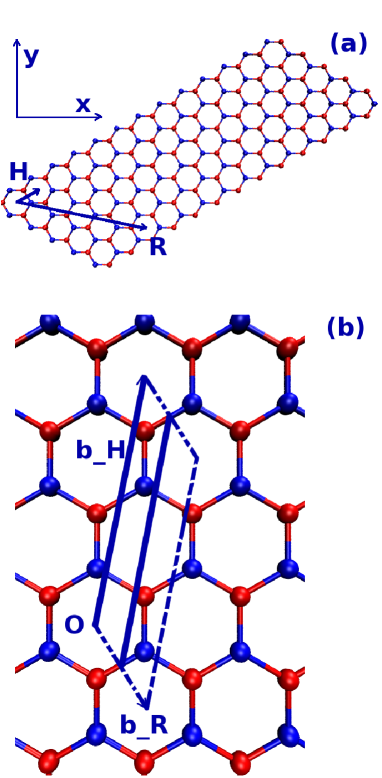
Figure 1: Graphene strip is described by a lattice vector $\vec{R}=n_{1}\vec{a}_{1}+n_{2}\vec{a}_{2}$. (a). Strip with $(n_{1},n_{2})=(4,2)$ and ($N_{H}$, $N_{R}$)=(12, 1); (b). The Brillouin zone for this special strip is two discrete segments (solid) in the reciprocal space.

II configuration

In graphene, the primitive lattice vectors are $\vec{a}_{1}$ and $\vec{a}_{2}$, with $|\vec{a}_{1}|=|\vec{a}_{2}|=\sqrt{3}b_{0}$. $b_{0}=1.42$ is the C-C bond length in graphene.Saito2 The corresponding reciprocal unit vectors are $\vec{b}_{1}=(\frac{2\pi}{3b_{0}},\frac{-2\pi}{\sqrt{3}b_{0}})$, $\vec{b}_{2}=(\frac{2\pi}{3b_{0}},\frac{2\pi}{\sqrt{3}b_{0}})$.

As shown in Fig. 1 (a), a strip in the graphene sheet can be described by a lattice vector $\vec{R}=n_{1}\vec{a}_{1}+n_{2}\vec{a}_{2}$. The real lattice vector $\vec{H}=p_{1}\vec{a}_{1}+p_{2}\vec{a}_{2}$ is introduced throughWhite : $n_{1}p_{2}-n_{2}p_{1}=N$ ($N$ is the greatest common divisor of $n_{1}$ and $n_{2}$). The strip is denoted by $N_{H}\vec{H}\times N_{R}\vec{R}$, where $N_{H}$ and $N_{R}$ are numbers of the periods in the directions along $\vec{H}$ and $\vec{R}$, respectively. Instead of $\vec{a}_{1}$ and $\vec{a}_{2}$, we use ($\vec{H}$, $\vec{R}/N$) as the basic vectors in the following, and $\vec{b}_{H}$ and $\vec{b}_{R}$ are their corresponding reciprocal unit vectors:

$$\vec{b}_{H}=\frac{1}{N}(-n_{2}\vec{b}_{1}+n_{1}\vec{b}_{2}),$$

$$\vec{b}_{R}=p_{2}\vec{b}_{1}-p_{1}\vec{b}_{2}.$$

Any wave vector in the reciprocal space can be written as:

$$\vec{k} = k_{H}\vec{b}_{H}+k_{R}\vec{b}_{R}.$$ (1)

Using the periodic boundary conditions, this strip has $N_{H}$ translational periods in the $\vec{H}$ direction and $N_{R}\times N$ translational periods in the $\vec{R}$ direction. As shown in Fig. 1 (b), the Brillouin zone for the graphene strip is $N_{R}\times N$ discrete segments, which are parallel or coincide with $\vec{b}_{H}$. The coordinates for the wave vectors on these lines areSaito2 ($k_{H}$, $k_{R}$)=($i/N_{H}$, $j/N_{R}N$), with $i=0,1,2,...,N_{H}-1$ and $j=0,1,2,...,N_{R}N-1$.

The graphene sheet is actually a strip in the limit of $N_{H}\longrightarrow\infty$ and $N_{R}\longrightarrow\infty$. In this case, the Brillouin zone for the strip, i.e., $N_{R}\times N$ discrete lines, turns to the two-dimensional Brillouin zone for the graphene.

III conductance formulas

The contribution of the phonon to the thermal conductance in the ballistic region is:Pendry ; Rego ; Wang3

$$\sigma(T)=\frac{1}{2\pi}\int_{0}^{\infty}T(\omega)\hbar\omega\frac{df}{dT}d\omega,$$

where $f(T,\omega)$ is the Bose-Einstein distribution function. $T(\omega)$ is transmission function. In the ballistic region, $T(\omega)$ is simply the number of phonon branches at frequency $\omega$.

From the above expression, the thermal conductance in the graphene strip can be written as:

$$\sigma(T) = \sum_{j=0}^{NN_{R}-1}\sum_{n=1}^{6}\sum_{\vec{v}_{n}^{\theta}>0}\frac{1}{2\pi}\int_{0}^{b_{H}}dk_{H}\times$$ (2)

$$\hbar\omega_{n}(\vec{k})\frac{df}{dT}v_{n}^{\theta}(\vec{k})T_{n}(\vec{k}),$$

where $\theta$ determines the direction of the thermal flux: $\vec{e}_{\theta}=(\cos\theta,\sin\theta)$. $\vec{k}=k_{H}\vec{b}_{H}+\frac{j}{NN_{R}}\vec{b}_{R}$ is the wave vector in the Brillouin zone of the strip, i.e., on the $N_{R}\times N$ discrete lines. The transmission function for a phonon mode $T_{n}(\vec{k})$ is assumed to be one.Wang1 $v_{n}^{\theta}(\vec{k})=\frac{\partial\omega_{n}(\vec{k})}{\partial k_{\theta}}$ is the group velocity of mode $(\vec{k},n)$ in $\vec{e}_{\theta}$ direction. The value of the group velocity can be accurately calculated through the frequency and the eigen vector of this phonon mode:Wang1 ; Wang2

$$v_{n}^{\theta}(\vec{k})=\frac{\partial\omega_{n}(\vec{k})}{\partial k_{\theta}}=\frac{\vec{u}_{n}^{\dagger}(\vec{k})\cdot\frac{\partial D}{\partial k_{\theta}}\cdot\vec{u}_{n}(\vec{k})}{2\omega_{n}(\vec{k})},$$ (3)

where $D$ is the dynamical matrix and $\vec{u}_{n}(\vec{k})$ is the eigen vector. Only those phonon modes with $\vec{v}_{n}^{\theta}>0$ contribute to the thermal conductance in the $\vec{e}_{\theta}$ direction.

In the two-dimensional graphene strip system, it is convenient to use conductance reduced by cross section: $\tilde{\sigma}=\sigma/s$, where $s=W\times h$ is the cross section. The thickness of the strip, $h=3.35$ Å, is chosen arbitrarily to be the same as the space between two adjacent layers in the graphite. The width for the strip is $W=N_{R}|\vec{R}|$, where, the thermal flux in the strip is set to be in the direction perpendicular to $\vec{R}$, i.e., $\vec{e}_{\theta}=\vec{b}_{H}/b_{H}$. We address a fact that the integral parameter ($k_{H}$) in Eq. (2) is the quantum number along the thermal flux direction.

The thermal conductance in $\vec{e}_{\theta}$ direction of the graphene can be obtained by:

$$\tilde{\sigma}(T) = \lim_{N_{R}\longrightarrow\infty}\frac{1}{Wh}\sigma(T).$$ (4)

IV calculation results and discussion

IV.1 graphene results

The phonon spectrum of graphene is calculated in the VFFM, which has been successfully applied to study the phonon spectrum in the single-walled carbon nanotubesMahan and multi-layered graphene systems.Jiang In present calculation, we utilize three vibrational potential energy terms. They are the in-plane bond stretching ($V_{l}$) and bond bending ($V_{BB}$), and the out-of-plane bond bending ($V_{rc}$) vibrational potential energy. The three force constants are taken from Ref. Jiang, as: $k_{l}$=305.0 Nm^-1, $k_{BB}$=65.3 Nm^-1 and $k_{BB}$=14.8 Nm^-1.

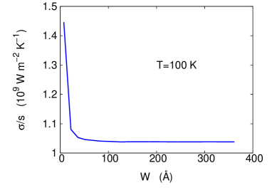
Figure 2: Convergence for the thermal conductance of the graphene strip with increasing width at temperature 100 K. In the large width limit ($W$$>$150Å) the thermal conductance of the strip can be considered as the thermal conductance value of graphene.

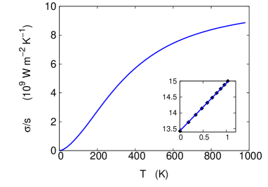
Figure 3: The thermal conductance of the graphene sheet v.s. temperature. Inset is $\log\tilde{\sigma}$ v.s. $\log T$ in extremely low temperature region. The calculated results (filled squares) can be fitted by function $f(x)=13.44+1.5x$ (blue line). It indicates that the thermal conductance has a $T^{1.5}$ dependence in this region.

Table 1: The dependence of the thermal conductance on group velocities of phonon modes. ‘b’ in the 2nd line is a fitting parameter (see text). In the 4th line, the down (up) arrow indicates the decreasing (increasing) of $\Delta\tilde{\sigma}$ when the corresponding phonon mode is excited more.

velocity	$\alpha$	$v_{2}$	$v_{3}$	$v_{4}$	$v_{5}$	$v_{6}$
sign($b$)	$-$	$-$	+	$-$	+	$-$
$\tilde{\sigma}\propto$	$\frac{1}{\sqrt{\alpha}}$	$\frac{1}{v_{2}}$	$\frac{1}{v_{3}}$	$v_{4}$	$v_{5}$	$v_{6}$
$\Delta\tilde{\sigma}$	$\downarrow$	$\downarrow$	$\uparrow$	$\uparrow$	$\downarrow$	$\uparrow$

IV.1.1 temperature dependence for thermal conductance

In Fig. 2, the temperature is 100 K and the direction angle for the thermal flux is $\theta=\pi/3$. It is shown that the thermal conductance for a strip decreases with increasing width. At about $W$=100 Å, the thermal conductance reaches a saturate value, which is actually the thermal conductance for the graphene. In the calculation, the width we used is about 300 Å, which ensures that the strip is wide enough to be considered as a graphene sheet.

In Fig. 3, the thermal conductance versus the temperature is displayed. In the low temperature region, the thermal conductance has a $T^{1.5}$ dependence. This is the result of the flexure mode in the graphene sheet, which has the dispersion $\omega=\alpha k^{2}$. In the very low temperature region, this mode makes the largest contribution to the thermal conductance. Its contribution to the thermal conductance isMingo $\tilde{\sigma}\propto T^{1.5}/\sqrt{\alpha}$, which can be seen from the figure in the low temperature region. At room temperature $T$=300 K, the value for the thermal conductance is about $4.4\times 10^{9}$ Wm^-2K^-1. This result agrees with the recent experimental value for the thermal conductance in the graphene.Balandin ; Ghosh In the experiment, the thermal conductivity is measured to be about $5.0\times 10^{3}$ Wm^-1K^-1 at room temperature. The distance for the thermal flux to transport in the experiment is $L$=11.5 $\mu$m. So the reduced thermal conductance can be deduced from this experiment as $\tilde{\sigma}=\frac{\sigma}{s}=\frac{\kappa}{L}=0.43\times 10^{9}$ Wm^-2K^-1. Our theoretical result is much larger than this experimental value. Because our calculation is in the ballistic region, while in the experiment, there is scattering on defects, edges or impurities and thus the transport is partially diffusive. At the high temperature limit $T=1000K$, our calculation gives the value 8.9 $\times 10^{9}$ Wm^-2K^-1, which is in consistency with the previous theoretical result.Mingo

IV.1.2 directional dependence for thermal conductance

As shown in Fig. 4, at $T$=100 K, the thermal conductance varies periodically with the direction angle $\theta$. The calculated results can be fitted very well by the function $f(\theta)=a+b\cos(6\theta)+c\cos(12\theta)$. The difference between the thermal conductance in the two directions with angle $\theta=0$ and $\pi$/2 is about 1.2$\times 10^{7}$Wm^-2K^-1. This difference is very stable for graphene strips with different width (see Fig. 5). At $T$=100 K, the lattice thermal conductance is about two orders larger than the electron thermal conductance.Saito So the experimental measured thermal conductance at $T$=100 K is mainly due to the contribution of the phonons. As a result, our calculated directional dependence of the lattice thermal conductance in the graphene can be carefully investigated in the experiment. In the following, we say that two quantities $Q_{1}=a_{1}+b_{1}\cos 6\theta$ and $Q_{2}=a_{2}+b_{2}\cos 6\theta$ have the same (opposite) dependence on $\theta$, if the signs of $b_{1}$ and $b_{2}$ are the same (opposite).

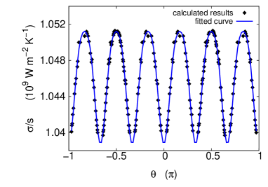
Figure 4: The direction dependence of thermal conductance. $\theta$ is the direction angle for the thermal flux. The calculated results (filled squares) are fitted by the function $f(x)=a+b\cos(6\theta)+c\cos(12\theta)$ with $a=1.0456\times 10^{9}$, $b=-6.237\times 10^{6}$ and $c=-9.642\times 10^{5}$.

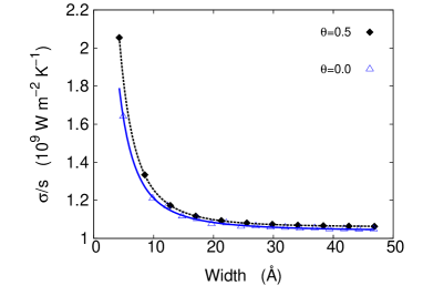
Figure 5: Thermal conductance in $\theta=0$ and $\pi/2$ directions versus width of graphene strip. Lines are guide to the eye.

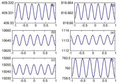
Figure 6: The coefficient and velocity of the six phonon spectrum around $\Gamma$ point in the Brillouin zone: (a). the coefficient of the out-of-plane acoustic mode with $\omega=\alpha k^{2}$ in the unit of $10^{-9}$ m²s^-1; (b)-(f). velocities of the other five phonon spectrum (from low frequency to high frequency), in the unit of $ms^{-1}$. The horizontal axises in all figures are the direction angle $\theta$ in the unit of $\pi$.

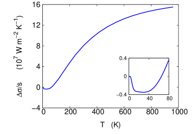
Figure 7: The difference of the thermal conductance between directions of $\theta=0$ and $\pi/2$ versus temperature. This quantity has an abundant temperature dependence. Inset is the enlarged figure for the low temperature region.

To find the underlying mechanism for this directional dependence for the thermal conductance, firstly we show in Fig. 6 the coefficient $\alpha$ for the flexure mode and the velocities for the other five phonon modes at the $\Gamma$ point. Interestingly, this coefficient and velocities are also directional dependent with the period $\pi/3$. Obviously, they can be fitted by function $f(\theta)=a+b\cos(6\theta)$. In Table 1, the sign of the fitting parameter $b$ for this coefficient and five velocities are listed, which can be read from Fig. 6. In the third line of Table 1, we list the contribution of the six phonon modes to the thermal conductance. If the three low frequency modes are excited, the thermal conductance is in inverse proportion to their velocities.Mingo While as can be seen from Eq. (4), the thermal conductance is proportional to the velocities for the three high frequency optically modes when they are excited. In each temperature region, there will be a key mode which is the most important contributor to the thermal conductance. The direction dependence of the velocity of this key mode determines the direction dependence of the thermal conductance.

We then further study the difference between the thermal conductance in two directions with $\theta=0$ and $\frac{\pi}{2}$: $\Delta\tilde{\sigma}=\tilde{\sigma}(\frac{\pi}{2})-\tilde{\sigma}(0)$. In the fourth line of Table 1, we display the effect of different modes on $\Delta\tilde{\sigma}$. It shows that $\Delta\tilde{\sigma}$ will decrease, if the first, second and fifth phonon modes are excited sufficiently with increasing temperature. The other three phonon modes have the opposite effect on the thermal conductance. The dependence of $\Delta\tilde{\sigma}$ on the temperature is shown in Fig. 7, where five different temperature regions are exhibited.

(1) [0, 4]K: In this extremely low temperature region, only the flexure mode is excited. This mode results in $\Delta\tilde{\sigma}<0$. Because the coefficient $\alpha$ depends on the direction angle $\theta$ very slightly, the absolute value of $\Delta\tilde{\sigma}$ is pretty small (see inset of Fig. 7).

(2) [4, 10]K: The second acoustic mode is excited in this temperature region. In respect that this mode has more sensitive direction dependence and favors to decrease $\Delta\tilde{\sigma}$, $\Delta\tilde{\sigma}$ decreases much faster than region (1).

(3) [10, 70]K: In this temperature region, the third acoustic mode begins to have an effect on the thermal conductance. This mode’s directional dependence is opposite of the previous two acoustic modes and it will increase $\Delta\tilde{\sigma}$. The competition between this mode and the other two acoustic modes slow down the decrease of the value $\Delta\tilde{\sigma}$ at temperature below $T$=40K. The third acoustic mode becomes more and more important with temperature increasing, and $\Delta\tilde{\sigma}$ begins to increase after $T$=40K as can be seen from the inset of Fig. 7.

(4) [70, 500]K: The third acoustic mode becomes the key mode in this temperature region. As a result, $\Delta\tilde{\sigma}$ changes into a positive value and keeps increasing.

(5) [500, 1000]K: In this high temperature region, the optical mode will also be excited one by one in the frequency order with increasing temperature. Since there are two optical modes (1st and 3rd optical modes) favors to increase $\Delta\tilde{\sigma}$, while only one optical mode (2nd optical mode) try to decrease $\Delta\tilde{\sigma}$, the competition result is increasing of $\Delta\tilde{\sigma}$ in the high temperature region.

$T$=100K is in region (4), where the direction dependence of the thermal conductance is controlled by the velocity of the third mode, so the dependence of $\tilde{\sigma}$ on $\theta$ in Fig. 4 is opposite to the dependence of velocity $v_{3}(\theta)$ in Fig. 6 (c).

IV.2 dimerite results

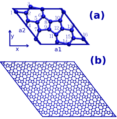
Figure 8: (Color online) Configuration for the dimerite. (a) is one unit cell for dimerite. There are 16 atoms in each unit cell. The length for the two unit vectors are 7.60 Åand 7.05 Å. The angle between them is 0.7 $\pi$. (b) shows 49 unit cells together.

The adatom defect is used as a basic block to manufacture a new carbon allotrope of graphene, named dimerite,Lusk2 and the relaxed configuration of this new material is investigated by a first principle calculation. The unit cell for the dimerite is shown in Fig. 8 (a), where the two basic unit vectors are $\vec{a}_{1}$ and $\vec{a}_{2}$, with $|\vec{a}_{1}|=7.60$ Å, and $|\vec{a}_{2}|=7.05$ Å. The angle between these two vectors is 0.7$\pi$. In each unit cell, there is a (7-5-5-7) defect, which leads to two anisotropic directions: the (7-7) direction and the (5-5) direction. (7-7) direction is from the center of a heptagon to the opposite heptagon, and the (5-5) direction is from the center of a pentagon to the neighboring pentagon. These two directions are perpendicular to each other, and corresponding to $\theta=0.4\pi$, 0.9$\pi$ respectively in Fig. 8 (a), where $\theta$ is the direction angle with respect to $x$ axis. From graphene to dimerite, the symmetry is reduced from $D_{6h}$ to $D_{2h}$.

IV.2.1 phonon dispersions in dimerite

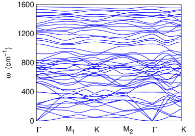
Figure 9: (Color online) Phonon spectrum for the dimerite along high symmetry lines in the Brillouin zone. Around $\Gamma$ point, there are low frequency optical modes with frequency about 200 cm^-1, which do not exist in pure graphene.

The phonon dispersion for the dimerite from the above VFFM is shown in Fig. 9. Similar with pure graphene, there are three modes with zero frequency. Two of them are the acoustic modes in the $xy$ plane. The other zero-frequency mode is a flexure mode with parabolic dispersion of $\omega=\beta k^{2}$. This flexure mode corresponds to the vibration in the $z$ direction. Different from the pure graphene, there are a lot of optical phonon modes with frequency around 150 cm^-1 in the dimerite.

IV.2.2 thermal conductance in dimerite

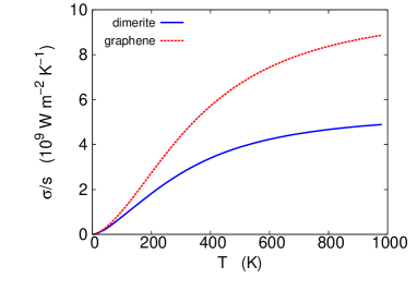
Figure 10: (Color online) The thermal conductance for the dimerite (blue solid line) and graphene (red dotted line) are compared in a large temperature region. The value of the dimerite is about 40$\%$ smaller than the graphene at room temperature.

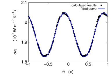
Figure 11: (Color online) The directional dependence for the thermal conductance of dimerite. The calculated results (filled squares) are fitted by function $f(x)=a+b\cos(2(\theta+c))$ with $a$=1.9$\times 10^{9}$, $b$=1.1$\times 10^{8}$, and $c$= 0.1$\pi$ (blue line).

In Fig. 10, we compare the thermal conductance of the dimerite with the graphene. At room temperature, the thermal conductance of the dimerite is about 40$\%$ smaller than the graphene. As can be seen from Fig. 11, the thermal conductance in the dimerite is more anisotropic than graphene. The calculated results can be best fitted with function $f(x)=a+b\cos(2(\theta+c))$ with a=1.9$\times 10^{9}$, b=1.1$\times 10^{8}$, and c= 0.1$\pi$. The thermal conductance has a minimum value at $\theta=0.4\pi$, and maximum value at $\theta=0.9\pi$. As mentioned previously, the directions with $\theta=0.4\pi$, 0.9$\pi$ are the (7-7) and the (5-5) directions, respectively. So, the thermal conductance in (5-5) direction is 12$\%$ larger than (7-7) direction, which is about one order larger than that of the pristine graphene. We expect this anisotropic effect detectable experimentally if the precision in the current experiment can be improved.

V conclusion

In conclusion, we have calculated the phonon thermal conductance for graphene in the ballistic region, by considering the graphene as the large width limit of graphene strips. The calculated value for the thermal conductance at room temperature is comparable with the recent experimental results, while at high temperature region our results are consistent with the previous theoretical calculations. We have found that the thermal conductance is directionally dependent and the reason is the directional dependence of the velocities of different phonon modes, which can be excited in the frequency order with increasing temperature. By breaking the $D_{6h}$ symmetry in graphene, we can see more obvious anisotropic effect of the thermal conductance as demonstrated by dimerite.

We have following two further remarks:

(1). Since the anisotropic effect of thermal conductance in graphene is small (1$\%$), it requires high accuracy in the calculation of phonon mode’s group velocity to see this anisotropic effect. Thanks to the superiority of the VFFM, we can derive an analytic expression for the dynamical matrix and calculate accurately the value of the group velocity following Eq. (3). Thus we can obtain the 1$\%$ anisotropic effect in graphene as discussed in this manuscript. We also used the Brenner empirical potential implemented in the “General Utility Lattice Program” (GULP)Gale to calculate the phonon dispersion and group velocity in graphene. For lack of analytic expression for the dynamical matrix, we find that the accuracy is not high enough for the group velocity and it is difficulty to see this anisotropic effect.

(2). From symmetry analysisBorn , when thermal transport is in the diffusive region where the Fourier’s law exists, the $D_{6h}$ symmetry of graphene constrains the thermal conductivity to be a constant value. So the anisotropic effect in graphene can not be seen if the thermal transport is in the diffusive region, yet it can only be seen in the ballistic region as discussed in this manuscript. But the situation changes in dimerite, where the $D_{6h}$ symmetry is broken into $D_{2h}$. The $D_{2h}$ symmetry does not constrain the thermal conductivity to be a constant value even the Fourier’s law is valid. So we can expect to see the isotropic effect in the dimerite both in the ballistic and diffusive region.

References

- (1) K. S. Novoselov and A. K. Geim, Nature Materials 6, 183 (2007).
- (2) Y. Zhang, Y. W. Tan, H. L. Stormer, and P. Kim, Nature 438, 201 (2005).
- (3) K. S. Novoselov, Z. Jiang, Y. Zhang, S. V. Morozov, H. L. Stormer, U. Zeitler, J. C. Maan, G. S. Boebinger, P. Kim, and A. K. Geim, Science 315, 1379 (2007).
- (4) A. A. Balandin, S. Ghosh, W. Bao, I. Calizo, D. Teweldebrhan, F. Miao, and C. N. Lau, Nano. Lett 8, 902 (2008).
- (5) S. Ghosh, I. Calizo, D. Teweldebrhan, E. P. Pokatilov, D. L. Nika, A. A. Balandin, W. Bao, F. Miao, and C. N. Lau, Appl. Phys. Lett. 92, 151911 (2008).
- (6) S. Stankovich, D. A. Dikin, G. H. B. Dommett, K. M. Kohlhaas, E. J. Zimney, E. A. Stach, R. D. Piner, S. T. Nguyen, and R. S. Ruoff, Nature 442, 282 (2006).
- (7) C. Stampfer, E. Schurtenberger, F. Molitor, J. Güttinger, T. Ihn and K. Ensslin, Nano Lett., 8, 2378 (2008).
- (8) D. Gunlycke, D. A. Areshkin, J. Li, J. W. Mintmire, and C. T. White, Nano Lett., 7, 3608 (2007).
- (9) B. Standley, W. Z. Bao, H. Zhang, J. H. Bruck, C. N. Lau and M. Bockrath, Nano Lett., 8, 3345 (2008).
- (10) P. Blake, P. D. Brimicombe, R. R. Nair, T. J. Booth, D. Jiang, F. Schedin, L. A. Ponomarenko, S. V. Morozov, H. F. Gleeson, E. W. Hill, A. K. Geim, K. S. Novoselov, Nano Lett., 8, 1704 (2008).
- (11) M. T. Lusk and L. D. Carr, arXiv: 0809.3160v1.
- (12) C. T. White, D. H. Robertson, and J. W. Mintmire, Phys. Rev. B 47, 5485 (1993).
- (13) G. D. Mahan and G. S. Jeon, Phys. Rev. B 70, 075405 (2004).
- (14) N. Mingo and D. A. Broido, Phys. Rev. Lett. 95, 096105 (2005).
- (15) R. Saito, G. Dresselhaus, and M. S. Dresselhaus, Physical Properties of Carbon Nanotubes (Imperial College Press, 1998).
- (16) J. B. Pendry, J. Phys. A 16, 2161 (1983).
- (17) L. G. C. Rego and G. Kirczenow, Phys. Rev. Lett. 81, 232 (1998).
- (18) J.-S. Wang, J. Wang, and J. T. Lü, Eur. Phys. J. B, 62, 381 (2008).
- (19) J. Wang and J.-S. Wang, Appl. Phys. Lett. 88, 111909 (2006).
- (20) J. Wang and J.-S. Wang, J. Phys.: Condens. Matter 19 (2007).
- (21) J. W. Jiang, H. Tang, B. S. Wang, and Z. B. Su, Phys. Rev. B 77, 235421 (2008).
- (22) K. Saito, J. Nakamura, and A. Natori, Phys. Rev. B 76, 115409 (2007).
- (23) J. D. Gale, JCS Faraday Trans., 93, 629 (1997).
- (24) M. Born and K. Huang, Dynamical Theory of Crystal Lattices (Oxford University Press, Oxford, 1954).
- (25) D. L. Nika, E. P. Pokatilov, A. S. Askerov, and A. A. Balandin, Phys. Rev. B 79, 155413 (2009).