Analysis of Galactic late-type O dwarfs:
more constraints on the weak wind problem^,

Abstract

Aims. To investigate the stellar and wind properties of a sample of late-type O dwarfs in order to address the weak wind problem.

Methods. Far-UV to optical spectra of five Galactic O stars were analyzed: HD 216898 (O9IV/O8.5V), HD 326329 (O9V), HD 66788 (O8V/O9V), $\zeta$ Oph (O9.5Vnn), and HD 216532 (O8.5V((n))). We used a grid of TLUSTY models to obtain effective temperatures, gravities, rotational velocities, and to identify wind lines. The wind parameters of each object were obtained by using expanding atmosphere models from the CMFGEN code.

Results. We found that the spectra of our sample have mainly a photospheric origin. A weak wind signature is seen in C iv $\lambda\lambda$1548,1551, from where mass-loss rates consistent with previous CMFGEN results regarding O8-O9V stars were obtained ($\sim 10^{-10}-10^{-9}$ M_⊙ yr^-1). A discrepancy of roughly 2 orders of magnitude is found between these mass-loss rates and the values predicted by theory ($\dot{M}_{Vink}$), confirming a breakdown or a steepening of the modified wind momentum-luminosity relation at log $L_{\star}/L_{\odot}\lesssim 5.2$. We have estimated the carbon abundance for the stars of our sample and concluded that its uncertainty cannot cause the weak wind problem. Upper limits on $\dot{M}$ were established for all objects using lines of different ions, namely, P v $\lambda\lambda$1118,1128, C iii $\lambda 1176$, N v $\lambda$1239,1243, Si iv $\lambda\lambda$1394,1403, and N iv $\lambda$1718. All the values obtained are also in disagreement with theoretical predictions, bringing support to the reality of weak winds. Together with C iv $\lambda\lambda$1548,1551, the use of N v $\lambda$1239,1243  results in the lowest mass-loss rates: the upper limits indicate that $\dot{M}$ must be less than about -1.0 dex $\dot{M}_{Vink}$. Regarding the other transitions, the upper limits obtained still point to low rates: $\dot{M}$ must be less than about $(-0.5\pm 0.2)$ dex $\dot{M}_{Vink}$. We studied the behavior of the H$\alpha$ line with different mass-loss rates. For two stars, only models with very low $\dot{M}$’s provide the best fit to the UV and optical spectra. We explored ways to fit the observed spectra with the predicted mass-loss rates ($\dot{M}_{Vink}$). By using large amounts of X-rays, we verified that few wind emissions takes place, as in weak winds. However, unrealistic X-rays luminosities had to be used (log $L_{X}/L_{Bol}\gtrsim-3.5$). The validity of the models used in our analyses is discussed.

1 Introduction:

Massive stars of spectral types O and B play an extremely important role in astrophysics. They possess high effective temperatures ($T_{eff}>10$kK), intense ionizing radiation fields and often strong mass-losses through stellar winds, making their description considerably difficult for atmosphere and stellar evolution models. These stars are known to be progenitors of fascinating objects such as Red Supergiants (RSGs), Luminous Blue Variables (LBVs), Wolf-Rayet stars (W-Rs), and thus also of some of the most energetic phenomena in the Universe, i.e., of type II supernovae and some $\gamma$-ray bursts (Massey 2003; Woosley & Bloom 2006). They also heavily affect their host galaxies by transferring momentum, energy and enriched chemical elements to the interstellar medium (Abbott 1982; Freyer et al. 2003).

Although they have been studied for decades, the properties, origin and evolution of OB stars still present several observational and theoretical challenges. The dependency of their mass-loss rates ($\dot{M}$) on the metallicity ($Z$) for example, as well as their effective temperatures and wind structure (e.g. clumping) have been continuously debated in the literature during the last years (see for example Vink et al. 2001; Martins et al. 2002; Bouret et al. 2005; Puls et al. 2006; Crowther et al. 2006).

Among several interesting issues currently under discussion (for a review see Puls 2008; Hillier 2008), one that have been receiving special attention is the so-called weak wind problem, which is posed by late-type O dwarf stars. From a qualitative point of view, O stars with weak winds present mainly an absorption spectrum, with the exception being a very few weak wind lines. In fact, often only a weak C iv $\lambda\lambda$1548,1551  in P-Cygni is seen. In contrast, mid- and early O dwarfs can present P-Cygni profiles in lines such as C iv $\lambda\lambda$1548,1551, N iv $\lambda$1718, N v $\lambda$1239,1243  or O v $\lambda$1371  (see e.g. Snow et al. 1994; Escolano et al. 2008). Quantitatively, weak wind stars are defined as having mass-loss rates of less than about $10^{-8}$ M_⊙ yr^-1. Bouret et al. (2003) were one of the first to suggest such low values after analyzing O dwarfs in the H II region NGC 346 in the SMC. The spectra of three objects of their sample could only be reproduced by models using mass-loss rates of $\sim 10^{-10}$ to $10^{-9}$ M_⊙ yr^-1. Similar results were found by Martins et al. (2004) for 4 O dwarfs in the compact star formation region N81, also in the SMC. Later, weak winds were also found in some Galactic O dwarfs, demonstrating that they are not result of an environmental (i.e. $Z$) effect (Martins et al. 2005). Despite these findings, as we will discuss later, very low $\dot{M}$ values are not of general consensus.

There are interesting questions that O stars with very low mass loss rates rise. From the stellar evolution point of view, it is well known that mass-loss is a fundamental ingredient in the models. Very different values for this parameter can alter considerably the way the stars evolve. For example, mass-loss can change the rotational structure of a star (decreasing surface and internal velocities; $\Omega_{r}$) due to removal of angular momentum combined with internal transport mechanisms (Meynet & Maeder 2000). Very low $\dot{M}$’s might thus imply that stars can keep high rotational velocities and get closer to break-up velocities. Low mass-loss rates can also change the way we understand the evolution in the LBV and W-R phases. The total mass lost from the Main Sequence prior the LBV phase can be much less than currently thought. As a consequence, in order to be consistent with observed masses of hydrogen deficient W-R stars, other intense mass-loss mechanisms must occur (e.g. continuum driven giant eruptions in the LBV phase) and/or evolutionary time scales (e.g. of the WNL phase) must be changed (see Smith & Owocki 2006; van Marle et al. 2008). Given these considerations, to be sure that weak winds exist is now essential.

From the radiative wind theory point of view, the low mass-loss rates obtained for late type O dwarfs also present challenges. While the last, state-of-art theoretical $\dot{M}$ predictions of Vink et al. (2000; 2001; $\dot{M}_{Vink}$) present a good match for objects with log $L/L_{\odot}$ greater than about 5.2 (neglecting clumping), for late-type, less luminous objects a discrepancy of even a factor of 100 can be found (Martins et al. 2005). Late O dwarfs data also suggest a breakdown of the modified wind momentum luminosity relation (WLR; Kudrizki & Puls 2000) or at least a change in its slope (see Fig. 41 of Martins et al. 2005). All these facts constitute what is now called the weak wind problem .

A possible reason for the discrepancies aforementioned is that mass-loss rates determinations based on UV lines could be incorrect, as it was suggested by Mokiem et al. (2007). The use of only one UV diagnostic line (i.e. C iv $\lambda\lambda$1548,1551), the abundance of carbon, the effect of X-rays, and the wind ionisation structure derived from the models are claimed to be considerable sources of errors for the derivation of $\dot{M}$. This means that stronger winds could perhaps have been found if appropriate diagnostic tools were used/available. According to Mokiem et al. (2007), three objects which are supposed to be in the weak wind regime ($\zeta$ Oph, CygOB2#2, and HD 217086) actually do not show very low mass-loss rates (i.e. $\dot{M}$’s are consistent with theory) if H$\alpha$ is used as the diagnostic.

In order to clarify some of the issues described above and get more insight into the weak wind problem, we have analyzed in detail far-UV, UV and optical high-resolution spectra of five Galactic late-type O dwarf stars. Their stellar and wind physical parameters were obtained using the codes TLUSTY and CMFGEN (Hubeny & Lanz 1995; Hillier & Miller 1998). With this work, the number of O8-9V objects studied by means of state-of-art atmosphere models is increased considerably, since only six were previously analyzed (Repolust et al. 2004; Mokiem et al. 2005; Martins et al. 2005).

The remainder of this paper is organized as follows. In Section 2 we describe the way we have selected our targets and the observational material used. A description of the atmosphere codes and the adopted assumptions are given in Section 3. The analysis of each object of our sample is presented in Section 4. The derived stellar and wind parameters are presented later in Section 5 along with comparisons to previous results and theoretical predictions. In Section 6 we discuss the carbon abundance and its relation with the mass-loss rate. In Section 7 we present estimates for the mass-loss rates of the programme stars using other lines besides C iv $\lambda\lambda$1548,1551. In Section 8 we discuss the consequences of our findings and explore a way to have agreement with the observed spectra using the mass-loss rates predicted by theory. Section 9 summarizes the main results found in our study.

2 Target Selection and Observations:

Table 1: Observational Data of the Programme Stars.

			far-UV		UV		Optical
Star	Spectral Typea	V	Data Setb	Date	Data Set	Date	Instrument	Date
HD 216898	O9IV, O8.5V	8.04	F - A0510303	2000-08-03	SWP43934	1992-02-05	OHP/ELODIE	2004-08-29
HD 326329	O9V	8.76	F - B0250501	2001-08-09	SWP48698	1993-09-21	ESO/FEROS	2005-06-25
HD 66788	O8V, O9V	9.43	F - P1011801	2000-04-06	SWP49080	1993-11-03	ESO/FEROS	2004-12-22
$\zeta$ Oph	O9.5Vnn	2.56	C - C002	1972-08-29†	SWP36162	1989-04-29	OHP/ELODIE	1998-06-11
HD 216532	O8.5V((n))	8.03	F - A0510202	2000-08-02	SWP34226	1988-09-11	OHP/ELODIE	2005-11-10

• Spectral types come from Lesh (1968), Schild et al. (1969), Garrison (1970), Walborn (1973), and MacConnell & Bidelman (1976).

• Satellite used to obtain spectra: F=FUSE and C=Copernicus.

• Orbits #115-247 (Snow et al. 1977).

The Galactic stars claimed to have weak winds in the literature belong mainly to the O8, O8.5, O9, and O9.5V spectral types (hereinafter we refer to them simply as O8-9V). In order to carry out our investigation, we initially selected a sample of several objects belonging to these classes by using the Galactic O Star Catalog (Maìz-Apellániz et al. 2004; hereinafter the GOS Catalog). Various stars were previously observed by our group (at optical wavelengths), and we have retrieved the spectra of some others from public available archives. After a first examination, we neglected all those objects that presented a peculiar spectrum. This included for example stars known to be binaries (having contamination or known to show strong variability in the spectrum) or ON8-9V objects. Due to our aim to study wind lines, we have drastically decreased the number of objects by considering only the ones having both UV and far-UV data. Furthermore, we have also neglected the stars in common with the work of Martins et al. (2005), since they were analyzed with the same atmosphere code utilized here (CMFGEN). In the end, we have chosen a subsample of five objects, listed in Table 1.

2.1 Optical Data:

For the optical, we used data collected with the MPI 2.2m telescope, located at the European Southern Observatory (ESO), in La Silla, Chile. The high resolution (R=48000) FEROS spectrograph was used and the total wavelength coverage is $\sim$ 4000-9000Å. The spectra were wavelength calibrated and optimally extracted using the available pipeline (for more details see Kaufer et al. 1999).

We have also used spectra obtained with the 1.93m telescope at the Observatoire de Haute-Provence, France, using ELODIE. This spectrograph has a resolving power R = 42000 in the wavelength range $\sim$3900-6800Å. The exposure times were set to yield a signal-to-noise (S/N) ratio above 100 at about 5000Å. The data reduction, the order localization, background estimate/subtraction, and wavelength calibration, were performed using the available pipeline (see Baranne et al. 1996). Each order was normalized by a polynomial fit to the continuum, specified by carefully selected continuum windows. At last, we have merged the successive orders to reconstruct the full spectrum. The spectrum of $\zeta$ Oph was obtained from the ELODIE archive (see Moultaka et al. 2004 for more details). We have retrieved small portions of its pipeline treated spectrum and then normalized them using polynomial fits.

2.2 Ultraviolet Data:

Different sources were used for the UV and far-UV data. We have retrieved spectra from the IUE and FUSE satellites using the Multimission Archive at STScI. Regarding the IUE data, the high resolution SWP mode was preferred ($\sim 0.2$Å), but spectra in the LWP/LWR region were also used to help in the determination of reddening parameters (R and E(B-V)). Regarding the FUSE data, we have relied only on the LiF2A channel, which comprises the $\sim 1087$-$1182$Å  interval. Spectra of a same object were co-added and smoothed with a five point average for better signal-to-noise ratio (S/N) and clarity. Although small, the LiF2A region provided two very useful features for our study, namely, P v $\lambda\lambda$1118,1128  and C iii $\lambda 1176$  (see Section 7.1). We have avoided other FUSE channels covering wavelengths less than $\sim 1087$Å  due to severe interstellar contamination. For one object of our sample, $\zeta$ Oph, there is no FUSE data available. Therefore, we have used far-UV data obtained with the Copernicus (“OAO-3”) satellite. The spectrum was retrieved from the Vizier Service and normalized “by eye”.

3 Models and Assumptions:

In order to obtain the stellar and wind parameters of the stars of our sample we have used the well known atmosphere codes TLUSTY (Hubeny & Lanz 1995) and CMFGEN (Hillier & Miller 1998). The TLUSTY code adopts a plane-parallel geometry, assumes hydrostatic and radiative equilibrium, and a non-LTE treatment including line-blanketing is taken into account. As such, it is suitable only to model lines that are not formed in a stellar wind, i.e., of photospheric origin. On the other hand, the radiative transfer and statistical equilibrium equations in CMFGEN are solved in a spherically symmetric outflow. The effect of line-blanketing is also taken into account, via a super-levels formalism (for more details see Hillier & Miller 1998). For the outflow we assume a $\beta$ velocity law which connects smoothly (at depth) with a hydrostatic structure provided by TLUSTY.

3.1 Methodology:

To start our analysis, we used a new grid of TLUSTY model atmospheres based on the OSTAR2002 grid (Lanz & Hubeny 2003). The new grid uses finer sampling steps in effective temperature ($1000K$) and surface gravity (0.2 dex), updated model atoms (for Ne and S ions, C iii, N ii, N iv, O ii, and O iii), and additional ions (Mg ii, Al ii, Al iii, Si ii, and Fe ii; see Lanz & Hubeny 2007). In order to derive $T_{eff}$, we have used mainly He i $\lambda$4471  and He ii $\lambda$4542  as diagnostic lines, but fits to other transitions such as He i $\lambda$4713  and He ii $\lambda$4686  were also checked for consistency. Typical errors for $T_{eff}$ range from 1 to $2kK$. Our derivation of log $g$ was based on the fit to the H$\gamma$ wings. For this parameter, the uncertainty varies from 0.1 to 0.2 dex, depending on the object. The rotational velocities ($vsini$) were adopted from previous studies (e.g. Penny 1996; Howarth et al. 1997) and/or refined/estimated from the fitting process when necessary. After we have derived the basic photospheric properties (i.e. $vsini$, log $g$, and $T_{eff}$) we have switched to CMFGEN to continue our investigation. As in previous studies, we noted a good agreement between TLUSTY and CMFGEN (e.g. Bouret et al. 2003). In general, conspicuous discrepancies were sorted out when we have increased the number of species or atomic levels and/or super-levels in CMFGEN.

Once effective temperatures were obtained, we have computed the radii by adopting luminosities typical of the O8-O9 dwarfs (see Table 4 of Martins et al. 2002), following the equation $R_{\star}=(L_{\star}/4\pi\sigma T^{4}_{eff})^{1/2}$. As we did not normalize the UV spectra, we have used the reddening parameters R and E(B-V) (following Cardelli et al. 1988) and the distance as free parameters to match the continuum in the IUE region. When a good fit was achieved, the R, E(B-V), and the distance used were considered representatives for the object in question. The values obtained were generally consistent with the ones estimated in the literature (see Sect. 4). Whenever a large discrepancy was encountered, we have revised our adopted $L_{\star}$ and hence $R_{\star}$, keeping $T_{eff}$ constant. A reasonable agreement is found between the final models and the observed absolute fluxes in the UV. In some cases however, local scalings of the theoretical continuum had to be made.

The two main wind parameters to be obtained are the mass-loss rate and the terminal velocity. Ideally, the determination of the mass-loss rates should be done by fitting different (sensitive) P-Cygni and emission lines in the optical (e.g. H$\alpha$) and in the UV (e.g. C iv $\lambda\lambda$1548,1551, N v $\lambda$1239,1243, Si iv $\lambda\lambda$1394,1403). In the case of late-type O dwarfs however, most of these wind transitions are absent and the best estimator of $\dot{M}$ is C iv $\lambda\lambda$1548,1551. Regarding the velocity structure, we have assumed $\beta=1$ for all our models. Initial tests with $\beta$ ranging from 0.8 to 1.6 did not improve the quality of the C iv $\lambda\lambda$1548,1551  fits. The terminal velocity ($v_{\infty}$) is a very difficult parameter to obtain for O8-O9V stars, since there are no clear, saturated P-Cygni profiles. We have chosen to first use previous $v_{\infty}$ estimates in the literature and then change its value from the fits, if needed. When such estimates were not available, we have started our models assuming $v_{\infty}$ values between 1300-1700 km s^-1. We conservatively assume the uncertainty in this parameter to be about 500 km s^-1. Regarding the mass-loss rate, we consider a conservative uncertainty of $\sim$ 0.7 dex, following the analysis performed by Martins et al. (2005).

Table 2: Atomic Data Used in the CMFGEN Models.

Ion	Basic Models		Full Models
	$\#$ levels	$\#$ super-levels	$\#$ levels	$\#$ super levels
H i	30	30	30	30
He i	69	69	69	69
He ii	30	30	30	30
C ii	22	22	338	104
C iii	243	99	243	217
C iv	64	64	64	64
N iii	287	57	287	57
N iv	70	44	70	44
N v	49	41	49	41
O ii	296	53	340	137
O iii	115	79	115	79
O iv	72	53	72	53
Ne ii	-	-	242	42
Mg ii	-	-	65	22
Al iii	-	-	65	21
Si iii	-	-	45	25
Si iv	33	22	33	22
P v	62	16	62	16
S iv	-	-	142	51
S v	-	-	216	33
Fe iii	-	-	607	65
Fe iv	1000	64	1000	64
Fe v	1000	45	1000	45

We have assumed a fixed microturbulence $\xi_{t}$ of 15 km s^-1 in the co-moving computation of our models. The CMFGEN code allows however a description of a depth dependent microturbulent velocity when passing to the observer’s frame, following the equation $\xi(r)=\xi_{min}+(\xi_{max}-\xi_{min})v(r)/v_{\infty}$. We have fixed $\xi_{min}$ at 5 km s^-1 (near the photosphere) and for $\xi_{max}$ we have assumed a value of $0.1v_{\infty}$. As it was already reported in previous studies, we noted that slightly different values for these parameters do not present significant changes in the spectrum.

We have used two sets of atomic data for CMFGEN in our study. The first fits/models to the observed spectra, tests, and the exploration of higher mass-loss rates (Section 7) were done using basic models, i.e., models with a reduced number of species and levels/super-levels. For our final model for each object, a more complete (full) set was used. In total, 4.5GB (2GB) of memory space (RAM) was required to compute each full (basic) model. The details of the atomic data are shown in Table 2. This approach could save a lot of computational time and resources, without compromising the results. The main difference between these two sets of data is the quality of the optical fit. Some lines could only be reproduced after the inclusion of additional species/ions (e.g. Mg ii $\lambda 4481$ and Si iii $\lambda 4553$) or by increasing the number of levels and/or super-levels. In the ultraviolet, only the 1850-2000Å  region is affected by the heavier data set (being better fitted), due to the inclusion of Fe iii. In other parts the changes are minor. A solar chemical abundance was adopted for all elements (following Grevesse & Sauval 1998). As it will be seen later in Section 4, it provides reasonable fits to the observations. In this paper, only the amount of carbon is investigated in detail (see Section 6), given its direct relation with the weak wind problem through C iv $\lambda\lambda$1548,1551.

3.2 Clumping and X-rays:

Currently, the effect of wind density inhomogeneities (i.e. clumping) is implemented in CMFGEN through a depth dependent volume filling factor $f=f_{\infty}+(1-f_{\infty})e^{v(r)/v_{cl}}$. The parameter $v_{cl}$ regulates the velocity where clumping starts to be important. At velocities higher than $v_{cl}$, $f$ converges quickly to $f_{\infty}$. With this description, the model is homogeneous near the photosphere. Because we have a lack of wind lines in the spectra of the stars studied here, we chose to not use clumping in our models, i.e., $f_{\infty}=1$. We stress that the use of clumping usually requires a decrease in the mass-loss rate of a (previously homogeneous final) model by a factor of $1/\sqrt{f_{\infty}}$, in order to fit (again) the observed spectra. Thus, the mass-loss in our final models can perhaps be overestimated by a factor of about three if $f_{\infty}\sim 0.1$ in the wind of these objects. In any case, to not use clumping means that we might be biased towards stronger winds.

CMFGEN also allows the inclusion of X-rays in the models to simulate the effects of shocks due to wind instabilities. The X-rays emissivity is basically controlled by a shock temperature plus a filling factor parameter and it is distributed throughout the atmosphere (see Hillier & Miller 1998 for details). The effects of X-rays in the atmosphere of O dwarfs were discussed in detail by Martins et al. (2005). These authors convincingly show that X-rays are not as important for early-type as they are for late-type O stars (see also Macfarlane et al. 1994). For early-type objects (denser winds), the ionisation and wind lines such as C iv $\lambda\lambda$1548,1551  do not present significant changes when X-rays are included. Only wind lines belonging to super-ions (O vi $\lambda\lambda$1032,1038  and to a lesser extent, N v $\lambda$1239,1243) are affected. In contrast, for late-type stars it is observed that the ionisation structure and the C iv $\lambda\lambda$1548,1551  line changes considerably. Because the ionisation is shifted to C v-vi, mass-loss rates about ten times stronger than in a model without X-rays are sometimes required to fit the observed C iv $\lambda\lambda$1548,1551  line. Due to this fact, as it is the case of non-clumped models, higher mass-loss rates are favored when X-rays are included. In this paper, we use a fixed shock temperature of $3\times 10^{6}K$ and the filling factor is chosen to keep log $L_{x}/L_{Bol}$ close to -7.0 (within $\pm 0.1$). We recall that a log $L_{x}/L_{Bol}$ of about -7.0 is the typical value observed (see e.g. Sana et al. 2006). For HD 326329 however, we used models with a higher ratio, in accord with the observations (log $L_{X}/L_{Bol}\sim-6.5$; Sana et al. 2006). For $\zeta$ Oph, we use a log $L_{X}/L_{Bol}\sim-7.3$ (Oskinova 2005; Oskinova et al. 2006).

4 Spectral Analysis:

In this section we present the analysis of our sample. A brief introduction about each object is made, followed by the presentation of our CMFGEN model fits to the UV and optical observed spectra. The discrepancies found are discussed and a comparison to previous results in the literature is given when necessary.

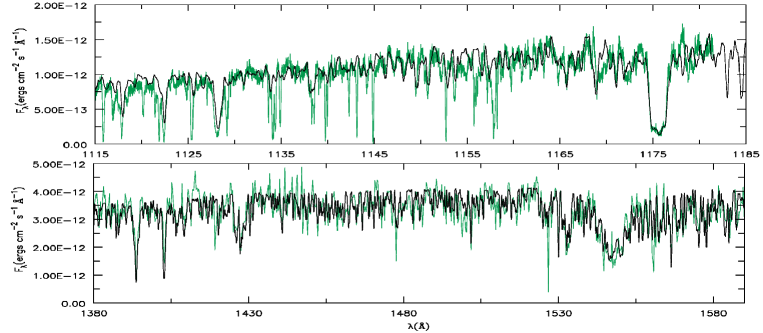
Figure 1: Ultraviolet spectra of HD 216898 (green/light gray line) and our final model (black line; log $\dot{M}=-9.35$).

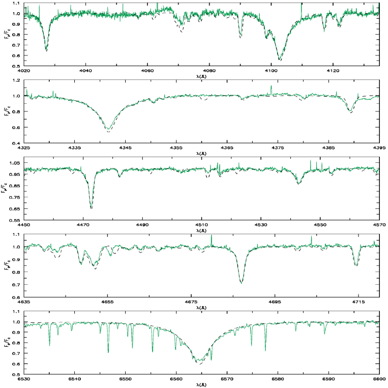
Figure 2: Optical spectrum of HD 216898 (green/light gray line) and our final model (black/dashed line).

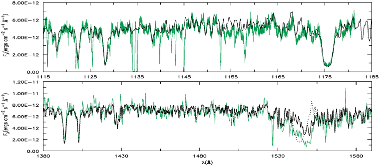
Figure 3: Ultraviolet spectra of HD 326329 (green/light gray line) and our final model (black line; log $\dot{M}=-9.22$). A model with a higher mass-loss rate is shown as a dotted line (log $\dot{M}=-8.55$; see text for more details).

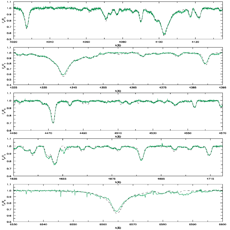
Figure 4: Optical spectrum of HD 326329 (green/light gray line) and our final model (black/dashed line).

Figure 5: Ultraviolet spectra of HD 66788 (green/light gray line) and our final model (black line; log $\dot{M}=-8.92$).

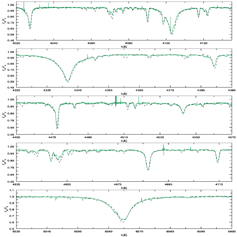
Figure 6: Optical spectrum of HD 66788 (green/light gray line) and our final model (black/dashed line).

Figure 7: Ultraviolet spectrum of $\zeta$ Oph (green/light gray line) and our final model (black line; log $\dot{M}=-8.80$). A model with a higher mass-loss rate is shown as a dotted line (log $\dot{M}=-8.30$; see text for more details).

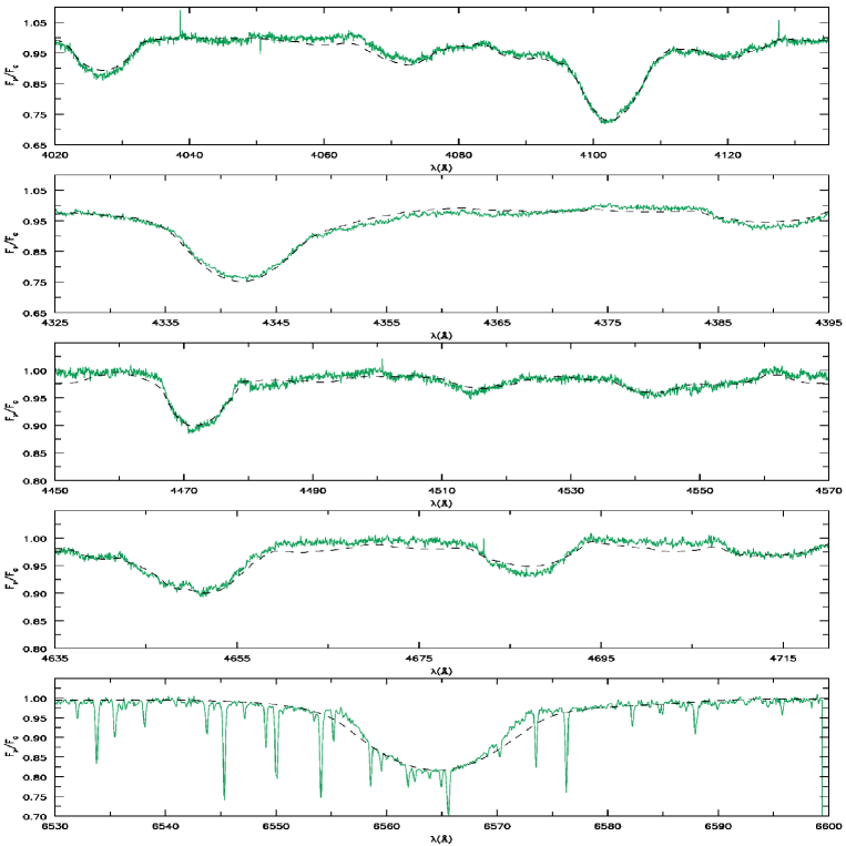
Figure 8: Optical spectrum of $\zeta$ Oph (green/light gray line) and our final model (black/dashed line).

Figure 9: Ultraviolet spectra of HD 216532 (green/light gray line) and our final model (black line; log $\dot{M}=-9.22$). A model with a higher mass-loss rate is shown as a dotted line (log $\dot{M}=-8.78$; see text for more details).

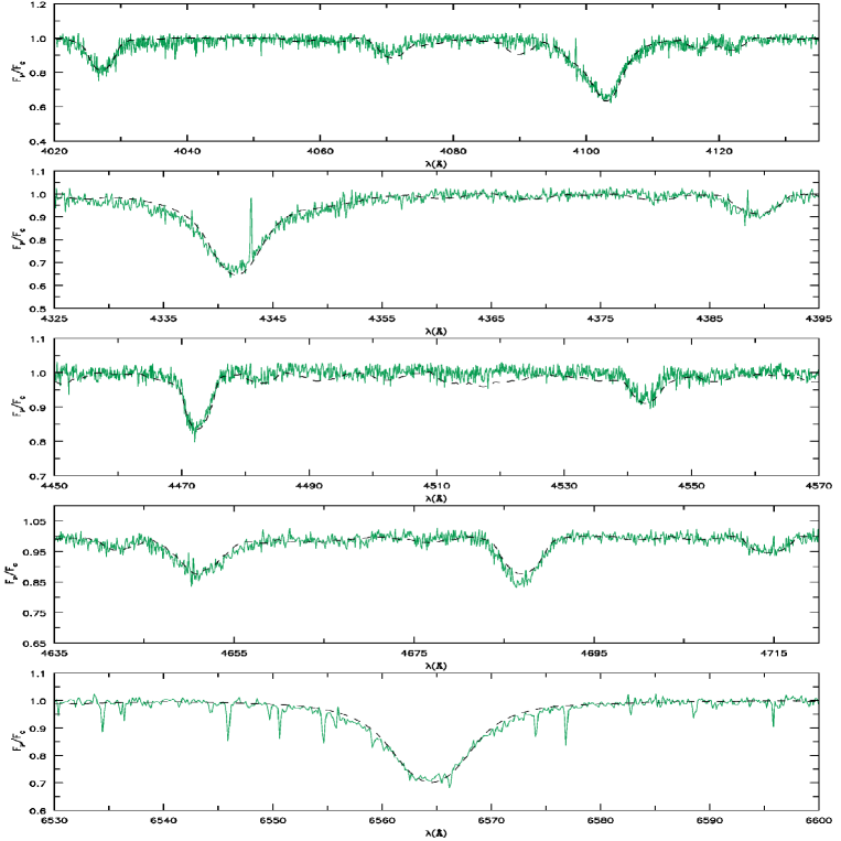
Figure 10: Optical spectrum of HD 216532 (green/light gray line) and our final model (black/dashed line).

4.1 HD 216898

HD 216898 belongs to the Cepheus OB3 association (Garmany & Stencel 1992). So far, no recent atmosphere models (i.e. unified, line-blanketed) were used to analyze this object. Its mass-loss rate was investigated two decades ago by Leitherer (1988), who could only establish an upper limit (log $\dot{M}<-6.97$) from the H$\alpha$ profile.

Our fits to the far-UV and UV spectra are presented in Figure 1. The E(B-V) and distance used are 0.7 and 1.1kpc, respectively. Four intense transitions can be noted in the FUSE region: P v $\lambda\lambda$1118,1128, Si iv $\lambda\lambda 1122,28$, and C iii $\lambda 1176$. The various narrow deep absorptions that are not reproduced by our models are of interstellar origin. As it can be seen in Figure 1 (bottom), our final model also fits correctly the main features of the IUE spectrum. In the 1380-1590Å  interval, Si iv $\lambda\lambda$1394,1403  and C iv $\lambda\lambda$1548,1551  are the most evident transitions. The other several absorptions observed we identified to be mainly due to Fe iv lines (an iron forest). We note that a TLUSTY model with the same photospheric parameters used in CMFGEN present a similar fit to the far-UV and UV, with the exception of C iv $\lambda\lambda$1548,1551. In TLUSTY, this doublet is seen as two well separated absorptions, while the observations show an extended blue feature that is only reproduced with CMFGEN, i.e., it is formed in the wind.

The mass-loss needed to fit C iv $\lambda\lambda$1548,1551  is log $\dot{M}=-9.35$. If we take the other physical parameters derived for this object ($T_{eff}$, $L_{\star}$, and $M_{\star}=gR_{\star}^{2}/G$) and use the recipe of Vink et al. (2000), we derive a predicted mass-loss rate of log $\dot{M}_{Vink}=-7.22$. A discrepancy of more than two orders of magnitude is observed ! If we use mass-loss rates higher than the one in our final model, a deeper blue absorption (with respect to the line center) and an intense emission starts to be seen, i.e., a more normal P-Cygni profile is developed, contrary to what is observed. On the other hand, lower $\dot{M}$’s slowly approach the photospheric prediction by TLUSTY, as expected.

In Figure 2 we present our fit to the optical spectrum of HD 216898. The five different spectral regions shown comprise the diagnostic lines used to derive the photospheric parameters (see Section 3.1). The effective temperature could be very well constrained. The He i $\lambda$4471$/$He ii $\lambda$4542  and He i $\lambda$4713$/$He ii $\lambda$4686  ratios are well reproduced with a $T_{eff}=(34\pm 1)kK$. H$\gamma$ has a reasonable fit but the model is somewhat stronger than the observed line. The same happens to H$\alpha$. Nevertheless, their wings are well matched with a log $g$ of 4.0 $\pm$ 0.1. Details regarding this last transition are discussed later in Section 7.2. Some of the most intense lines in Figure 2 are: He i $\lambda 4026$, H$\delta$, H$\gamma$, He i $\lambda 4388$, He i $\lambda$4471, He ii $\lambda$4542, C iii $\lambda 4647$, and C iii $\lambda 4650$ (with small contribution of O ii), He ii $\lambda$4686, He i $\lambda 4713$, and H$\alpha$. These same transitions are easily identified in the other objects of our sample - and in other typical O8-9V stars - that have $vsini$ less than about 100 km s^-1. For rapid rotators such as $\zeta$ Oph and HD 216532, several profiles are broadened/blended and in some cases we cannot distinguish individual transitions (see below). We highlight that the H$\alpha$ observed in HD 216898 is symmetric. Indeed, all model predictions are symmetrical for this line. However, as it is shown later, some objects present an asymmetric H$\alpha$ profile whose origin is not known.

4.2 HD 326329

HD 326329 is located in the NGC 6231 cluster, at the nucleus of the Sco OB1 association. It belongs to a resolved triple system (O9V+O9V+B0V; GOS Catalog), but it is probably a single star itself since it does not show photometric or spectroscopic variations (Garcia & Mermilliod 2001). So far, no atmosphere models were used to analyze its spectrum.

In Figure 3 we present our final model to the far-UV and UV observed spectra. From the IUE continua, we have derived a E(B-V) of 0.44 and a distance of 1.99 $kpc$, in agreement with the study of the NGC 6231 cluster made by Baume et al. (1999). As in the case of HD 216898, a good agreement is found in the FUSE spectral region. The P v $\lambda\lambda$1118,1128, Si iv $\lambda\lambda 1122,28$, and C iii $\lambda 1176$  lines are well reproduced. However, the IUE spectrum could not be entirely matched: the observed C iv $\lambda\lambda$1548,1551  is considerably deeper than in the model. We have tried several different tests to fix this discrepancy (e.g. changes in the $\beta$ velocity law; lower terminal velocities; increased turbulence), but they all turned out to be unsuccessful. We note that in the study of Martins et al. (2005) no such problem was found. The O9 dwarfs analyzed in their study present a C iv $\lambda\lambda$1548,1551  profile that was well reproduced by the models. We also emphasize that although there is only one IUE high resolution spectrum for HD 326329 (shown in Figure 3), model comparisons to the other few lower resolution IUE data available confirm the too deep/broad feature. Interestingly, one more star of our sample also present this characteristic, namely, HD 216532 (see below).

Despite the problem described above, we can still be confident about the mass-loss rate chose for HD 326329, log $\dot{M}$ = -9.22, within $\pm$0.7 dex. First, there is a lack of emission in the observed C iv $\lambda\lambda$1548,1551  P-Cygni profile, suggesting that $\dot{M}$ must be indeed low. When values for $\dot{M}$ higher than the one in our final model are used, a synthetic line with an intense (unobserved) emission and discrepant blue absorption appears (see Figure 3; dotted line). On the other hand, when lower mass-loss rates are used, C iv $\lambda\lambda$1548,1551  slowly turn into photospheric features, as the ones predicted in TLUSTY.

Our fit to the optical spectrum of HD 326329 is presented in Figure 4. The He i and He ii lines are well reproduced with a $T_{eff}=(31\pm 1)kK$. The fit to the H$\gamma$ wings gives a surface gravity (log $g$) of $3.9\pm 0.1$. Both $T_{eff}$ and log $g$ were previously estimated by Mathys et al. (2002) who found 31700$K$ and 4.6, respectively, by using $uvby\beta$ photometry. Although our derived temperature is compatible with their value, their higher log $g$ is not supported by our analysis. In fact, a log $g$ much higher than 4.0 is not expected for O stars (see e.g. Vacca et al. 1996; Martins et al. 2002). Although a fairly good agreement is found in several parts of the optical spectrum, we could not achieve a good fit to H$\alpha$. This line is weaker than in the model and is also asymmetric. Its blue wing has a “bump” which distorts the profile. This is not seen in the other hydrogen lines. We have not used H$\alpha$ to derive any stellar or wind parameters of the objects of our sample. However, we later discuss the effects that different mass-loss rates have on this line (see Section 7.2).

4.3 HD 66788

Figure 5 shows our fits to the ultraviolet spectrum of HD 66788. The C iv $\lambda\lambda$1548,1551  feature is reproduced with a mass-loss rate of log $\dot{M}$ = -8.92. This value is much lower than the one predicted, log $\dot{M}_{Vink}=-6.95$. The reddening and distance derived are E(B-V) = 0.22 and d = 4.8kpc. Although large, this distance is consistent with estimates encountered in the literature (Reed 1993; Kaltcheva & Hilditch 2000).

In Figure 6 we show our fit to the optical spectrum. The features found in HD 216898 and HD 66788 are very similar, suggesting similar photospheric parameters (see Section 4.1). Indeed, from our fits to the H$\gamma$ we derive a log $g=4.0\pm 0.1$, and from the He i $\lambda$4471  and He ii $\lambda$4542  lines we obtain a $T_{eff}=(34\pm 1)kK$, as in HD 216898. Their rotational velocities are also practically the same, about 60 km s^-1. We note that the H$\alpha$ line in HD66788 is slightly asymmetric. Although the overall agreement is reasonable, its blue wing has a weak absorption not predicted by the model.

4.4 $\zeta$ Oph

$\zeta$ Oph (also known as HD 149757) is a well studied runaway star which presents several interesting characteristics. It has been known for a long time to present different kinds of spectral variability, such as discrete absorption components in the UV (DACs), emission line episodes, and line profile variations (LPVs) (see e.g. Howarth et al. 1984; Reid et al. 1993; Howarth et al. 1993; Jankov et al. 2000; Walker et al. 2005). This object presents also a very high rotational velocity: $vsini$ values around 400 or even 500 km s^-1 were already reported in the literature (Walker et al. 1979; Repolust et al. 2004).

A reason to include $\zeta$ Oph in our sample, is that it is considered to have a $\dot{M}$ estimate based on H$\alpha$ which is in good agreement with the predictions of the radiative wind theory (Mokiem et al. 2005; 2007). Thus, it is interesting to check if a fit from the UV to the optical (including H$\alpha$) can be achieved with CMFGEN using a low $\dot{M}$. We stress however, that the very high rotational velocity presented by $\zeta$ Oph can bring some problems to the analysis. First, fast rotation can distort the shape and induce temperature and gravity variations through the stellar surface (see e.g. Frémat et al. 2005). Furthermore, it might imply that a stellar wind is not spherically symmetric. In such cases, 1D unified atmosphere models should be considered as an approximation. Another difficulty is that several features in the spectrum are broadened and sometimes blended. The analysis of diagnostic lines thus can present a greater difficulty than in the case of slower rotators.

Table 3: Stellar and Wind Parameters.

Star	HD 216898	HD326329	HD 66788	$\zeta$ Oph	HD 216532
Spec. type	O9IV, O8.5V	O9V	O8-9V	O9.5Vnn	O8.5V((n))
log g	4.0 $\pm$ 0.1	3.9 $\pm$ 0.1	4.0 $\pm$ 0.1	3.6 $\pm$ 0.2	3.7 $\pm$ 0.2
Teff (kK)	34 $\pm$ 1	31 $\pm$ 1	34 $\pm$ 1	32 $\pm$ 2	33 $\pm$ 2
vsini (km s-1)	60	80	55	400	190
log L/L⊙	4.73 $\pm$ 0.25	4.74 $\pm$ 0.10	4.96 $\pm$ 0.25	4.86 $\pm$ 0.10	4.79 $\pm$ 0.25
R⋆ (R⊙)	$6.7^{+2.3}_{-1.7}$	$8.0^{+1.1}_{-1.0}$	$8.7^{+3.0}_{-2.2}$	$9.2^{+1.7}_{-1.4}$	$7.5^{+2.7}_{-2.0}$
M⋆ ($M_{\odot}$)	17${}^{+15}_{-8}$	19${}^{+8}_{-6}$	26${}^{+23}_{-12}$	13${}^{+10}_{-6}$	12${}^{+14}_{-6}$
v∞ (km s-1)	1700 $\pm$ 500	1700 $\pm$ 500	2200 $\pm$ 500	1500 $\pm$ 500	1500 $\pm$ 500
log $\dot{M}$	-9.35 $\pm$ 0.7	-9.22 $\pm$ 0.7	-8.92 $\pm$ 0.7	-8.80 $\pm$ 0.7	-9.22 $\pm$ 0.7
log $\dot{M}_{Vink}$	-7.22	-7.38	-6.95	-6.89	-6.92
log $L_{x}/L_{Bol}$	-7.00	-6.69	-7.06	-7.31	-7.00
log L/$c^{2}$	-8.42	-8.41	-8.19	-8.29	-8.36
E(B-V)	0.7	0.44	0.22	0.36	0.72
R	3.5	3.1	2.8	2.9	3.5
distance (pc)	1100	1990	4800	146	1150

Our final model and the IUE spectrum of $\zeta$ Oph are shown in Figure 7. A distance of 146pc and an E(B-V)=0.36 was used for the continuum fit. Due to the high $vsini$ involved, the photospheric iron forest is considerably broadened. Despite weak, N v $\lambda$1239,1243  can be easily distinguished in the spectrum, as well as the C iii $\lambda 1176$  and the Si iv $\lambda\lambda$1394,1403  lines. As it is clear, the model is successful to reproduce the main UV features observed, but some discrepancies can be noted. The C iv $\lambda\lambda$1548,1551  line for example, could not be matched in detail; the synthetic line is slightly more intense and narrower than the observed one. A model with a mass-loss rate lower than in our final model does not solve the problem and has also a drawback in the N v $\lambda$1239,1243  fit. Also, a higher mass-loss rate implies in a stronger emission and blue absorption of the P-Cygni profile, in contrast with the observations (see Figure 7; dotted line). The rate used, log $\dot{M}=-8.80$, should be certain within a factor of three (i.e. $\sim$0.5 dex). This value is much lower than the one derived in the study of Mokiem et al. (2005). Using the FASTWIND code, and based on H$\alpha$, these authors derive log $\dot{M}(H\alpha)=-6.85$. Our value is also much lower than the one predicted according to Vink et al. (2000), log $\dot{M_{Vink}}=-6.89$. We come back to this question later in Section 7. Some other smaller discrepancies can be also seen in the Si iv $\lambda\lambda$1394,1403  line fit and on the $\sim 1550-1650$Å  interval. Despite our efforts, they could not be sorted out. Due to the very high rotational velocity presented by $\zeta$ Oph, future studies using 2D atmosphere models might be very useful to address some of these problems.

In Figure 8 we present our model to the optical spectrum. As we mentioned earlier, a high rotational velocity convolution is necessary to fit the broad features observed ($vsini\sim$ 400 km s^-1). Despite the high rotation, the effective temperature and surface gravity could be derived, but with a higher uncertainty than in the other objects of our sample. From the He i and He ii lines, we have obtained a $T_{eff}=(32\pm 2)kK$. From the H$\gamma$ profile we estimate a low surface gravity compared to the other objects: log $g=3.6\pm 0.2$. It should be kept in mind that this value should be regarded as an effective gravity, i.e., the gravity attenuated by rotation. A “centrifugal correction” can be applied in order to obtain the true gravity, according to the equation log $g_{true}=$ log $(g_{eff}+vsini^{2}/R_{\star})$ (see details in Repolust et al. 2004). For $\zeta$ Oph, we find a log $g_{true}$ of $\sim 3.8$. This correction however, neglects any distortion in the stellar shape. A treatment allowing the oblateness of the star was presented by Howarth & Smith (2001) for three fast rotators, including $\zeta$ Oph. These authors derived a polar (equatorial) gravity of $\sim$4.0 ($\sim$3.6), a polar (equatorial) radius of 7.5R_⊙ (9.1R_⊙), and an effective temperature of $\sim 34kK$. The radius obtained from our $T_{eff}$ and $L_{\star}$ is 9.2R_⊙. Therefore, our stellar parameters for $\zeta$ Oph are compatible to the equatorial values found by Howarth & Smith (2001). They also show agreement with other works in the literature (Repolust et al. 2004; Mokiem et al. 2005; Villamariz & Herrero 2005).

Turning our attention to H$\alpha$, we note that this line and a few others were observed to present emission episodes (in the form of double peaks) on different occasions (see e.g. Niemela & Mendez 1974; Ebbets 1981). However, in general, H$\alpha$ is observed to be a symmetric absorption, with an equivalent width ($W_{\lambda}$) of $(2.7\pm 0.4)$Å, and with a central depth of about 0.8 of the continuum intensity. These characteristics can be considered to represent $\zeta$ Oph’s quiescent spectrum (see Reid et al. 1993 and references therein). In our case, from the observed line we measure a $W_{\lambda}$ of $(3.0\pm 0.3)$Å  and the deepest part of the absorption is also at $\sim$0.8 of the continuum level, confirming a quiescent-like, i.e., normal spectrum. However, the profile presents narrower wings if compared to the one in our final model (see Figure 8, bottom). This problem can be also perceived in the model presented by Mokiem et al. (2005) using the FASTWIND code (see their Fig. 12). A decrease in the $vsini$ to 350 km s^-1 improves the fit to the wings, but the line center gets slightly deeper than observed. Such lower $vsini$ has also a negative effect in other optical lines such as H$\delta$ and H$\gamma$.

4.5 HD 216532

HD 216532 is a relatively fast rotator which belongs to the Cepheus OB3 association. According to Howarth et al. (1997) its $vsini$ is $\sim$190 km s^-1, a value that we confirm from our model fits. Leitherer (1988) have estimated its stellar parameters and derived an upper limit for the mass-loss rate from H$\alpha$, log $\dot{M}<-7.08$. The present study is the first to analyze quantitatively its far-UV to optical spectra.

Our fit to the far-UV and UV data is presented in Figure 9. For the E(B-V) and the distance, we inferred 0.72 and 1.15kpc, respectively. In the FUSE region, although the overall agreement is fair, some discrepancies can be noted. The observed P v $\lambda\lambda$1118,1128  and Si iv $\lambda\lambda 1122,28$ lines are deeper than in the model. Although we can see that the synthetic continuum is somewhat higher than the observed, the problem remains if we normalize the spectrum locally. Regarding the IUE spectrum, as in HD 326329, we could not fit the C iv $\lambda\lambda$1548,1551  line. Compared to the profiles found in HD 216898 and HD 66788, the C iv $\lambda\lambda$1548,1551  line in HD 216532 is broader and deeper. Nevertheless, the mass-loss rate of our final model, log $\dot{M}=-9.22$, should be certain within about $\pm$0.4 dex. Higher values result in P-Cygni profiles whose emissions are too strong, and this is not observed. An example is shown in Figure 9 (see the dotted line). As we already mentioned, lower mass-loss rates slowly change the C iv $\lambda\lambda$1548,1551  feature into two photospheric absorptions.

In Figure 10 we present the observed optical spectrum of HD 216532 along with our final model. It can be readily noted that the lines are broader if compared to the ones in HD 216898, HD 326329, and HD 66788, reflecting the relatively high $vsini$ of this object, $\sim$190 km s^-1. With an effective temperature of $\sim$33kK, we achieve a good match to the observed He i $\lambda$4471  and He ii $\lambda$4542  lines. To fit the H$\gamma$ profile, we have used a log $g$ of $3.7$.

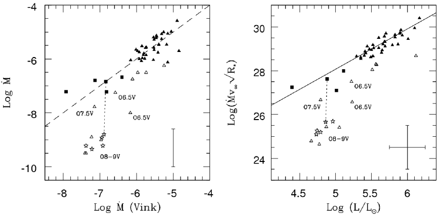
Figure 11: Comparison of our results to previous ones in the literature and theoretical predictions. The objects of our sample are represented by star symbols; the O dwarfs studied by Martins et al. (2005) by open triangles; the O and B stars compiled by Mokiem et al. (2007) that have log $L_{\star}/L_{\odot}\lesssim 5.2$ are represented filled squares and the ones with higher luminosities by filled triangles. Left panel: mass-loss rates compared to theoretical predictions ($\dot{M}_{Vink}$). The dashed line indicates a one-to-one relation. Right panel: modified wind momentum-luminosity relation (WLR). The solid line represents the best fit to the data in Mokiem et al. (2007). The dotted lines link the results obtained in this paper and in Mokiem et al. (2005) regarding the star $\zeta$ Oph. Low luminosity dwarfs (log $L_{\star}/L_{\odot}\lesssim 5.2$) in this paper and in Martins et al. (2005) are explicitly indicated by their spectral types (see text for more details).

5 Analysis of the Results:

In this section we summarize the results of our spectral analysis and make a comparison to previous works and theoretical predictions. The stellar and wind parameters obtained for each star of our sample are presented in Table 3. For comparison, we also list the theoretical mass-loss rates computed following the recipe of Vink et al. (2000), $\dot{M}_{Vink}$. Additional parameters such as the reddening and the distances are shown in the lower part of the table. Regarding the X-rays luminosities, we recall that for HD 216898, HD 66788, and HD 216532, we have fixed log $L_{X}/L_{Bol}$ at the canonical value, i.e. at $\sim-7.0$. For HD 326329 and $\zeta$ Oph, we chose $L_{X}/L_{Bol}$ ratios close to the ones recently observed (Oskinova 2005; Oskinova et al. 2006; Sana et al. 2006).

Overall, the stellar properties of our sample are quite homogeneous. The effective temperatures obtained range from $\sim$30-34$kK$, and the radii are between $\sim$7-9$R_{\odot}$. Regarding the surface gravities, the most different (lowest) values are presented by HD 216532 and $\zeta$ Oph. In both stars, the log $g$ measured should be interpreted as effective, i.e., they are attenuated by their fast rotation. These physical properties show a fair agreement with the latest calibration of Galactic O star parameters, regarding the O8-9V spectral types (see Martins et al. 2005b).

In order to better analyze the stellar and wind parameters derived, we also present our results in Figure 11, in two different ways: the mass-loss rates are compared to the theoretical predictions of Vink et al. (2000); and the wind parameters are used to construct the modified wind momentum luminosity relation (WLR): $(\dot{M}v_{\infty}\sqrt{R_{\star}})\times L_{\star}$. In each of these plots, we include the results of Martins et al. (2005) regarding eleven O dwarfs, as well as the data gathered by Mokiem et al. (2007) regarding O and B dwarfs, giants, and supergiants (see their Table A1). In order to simplify the analysis and exclude metallicity effects, only Galactic objects are considered.

In the plots presented in Figure 11, we can perceive the same basic result: the stars of our sample gather around the same places occupied by the four O8-9V stars studied in Martins et al. (2005), namely, $\mu$ Col, AE Aur, HD 46202, and HD 93028. This means that: (i) we have also found a discrepancy of roughly two orders of magnitude between the measured and the predicted mass-loss rates for our programme stars; (ii) the modified wind momentum-luminosity relation indeed shows a breakdown or a steepening below log $L_{\star}/L_{\odot}\sim 5.2$.

Regarding the brighter objects, i.e. with log $L_{\star}/L_{\odot}>5.2$, they follow reasonably well the theoretical expectations regarding the mass-loss rate. We remind that the four most luminous early-type dwarfs analyzed in the work of Martins et al. (2005) have clumped mass-loss rates. Thus, although they fall somewhat below the theoretical line in the log $\dot{M}$ x log $\dot{M}_{Vink}$ plot and below the fit to the data of Mokiem et al. (2007), they do not present a significant discrepancy if clumping is neglected.

The results derived by us and Mokiem et al. (2005) regarding the star $\zeta$ Oph are connected in Figure 11. The large difference observed is due to the different mass-loss rates derived. While we have log $\dot{M}=-8.80$ from the C iv $\lambda\lambda$1548,1551  line, Mokiem et al. (2005) derived log $\dot{M}=-6.84$ based on H$\alpha$, using the FASTWIND code. The other stellar and wind parameters determined in their study and ours are very similar. The radius, $T_{eff}$, and log $L_{\star}/L_{\odot}$ from this (their) paper are 9.2 (8.9) $R_{\odot}$, 32.1 (32) kK, and 4.86 (4.88), respectively. Regarding the wind terminal velocity, we (they) obtain 1500 (1550) km s^-1.

As we mentioned above, the objects of our sample and the four O8-9V stars analyzed in Martins et al. (2005) occupy about the same locus in the panels shown in Figure 11. It is interesting however to analyze their results for other stars having also low luminosities, i.e., with log $L_{\star}/L_{\odot}\lesssim 5.2$. Two objects in Martins et al. (2005) have a log $L_{\star}/L_{\odot}$ of about 5.2 ($\pm 0.2$ dex) and are classified as O6.5V stars: HD 93146 and HD 42088. Another object included in their study is HD 152590, an O7.5V with a log $L_{\star}/L_{\odot}\sim 4.8$. They fall relatively far from the O8-9V group in the plots in Figure 11. Contrary to the other four earlier O dwarfs, clumping was not used in their analysis. These three examples are suggestive that in stars of the spectral types O6.5V, O7V, and O7.5V, a decrease of the wind strength starts to be seen, culminating in the O8-9V classes.

Also at low luminosities are the following objects analyzed by Mokiem et al. (2005): Cyg OB2#2 (B1 I), $\tau$ Sco (B0.2V), 10 Lac (O9V), and HD 217086 (O7Vn) (see Figure 11; filled squares). They deserve special attention. In their case, their mass-loss rates clearly present better agreement to the theoretical predictions and also allow them to follow relatively well the WLR. Interestingly, their $\dot{M}$’s were obtained from the H$\alpha$ line. Given these and our UV based results, the origin of the weak wind problem can be thought to reside in the different mass-loss rates diagnostics employed. In fact, Mokiem et al. (2007) have suggested that the problem could be due to uncertainties in the UV method. We address and discuss these questions during the rest of the paper.

We emphasize that there are several other O8-9V stars with UV spectra similar to the ones found in our sample. Thus, it is likely that they possess similar wind properties, i.e., that the same basic results we have obtained will be achieved for them if we use the same methods of analysis.

6 The Carbon Abundance

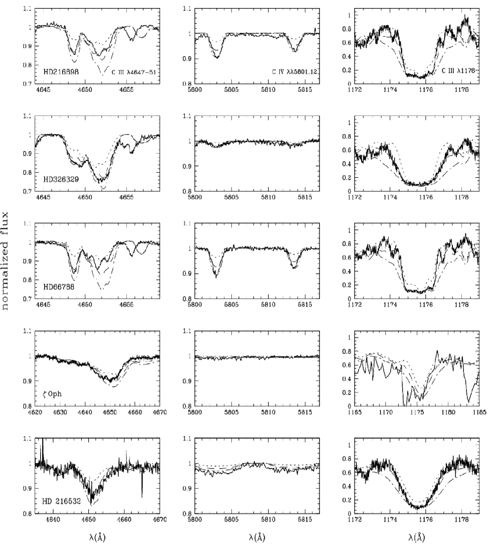
Figure 12: Determination of the carbon abundance in our programme stars. The observed spectra are indicated by solid line lines. The models shown have: 20% solar (0.2$\epsilon_{C_{\odot}}$; dotted line), solar ($\epsilon_{C_{\odot}}$; dashed line), and 3x the solar carbon abundance (3$\epsilon_{C_{\odot}}$;dashed-dotted line).

From the models, it can be easily seen that changes in the carbon abundance ($\epsilon_{C}$) affect the C iv $\lambda\lambda$1548,1551  profile. In fact, by choosing different combinations of $\dot{M}$ and $\epsilon_{C}$ we can get satisfactory fits to this feature, as long as its optical depth is kept constant, i.e., at the observed value. This can be seen more directly in terms of the Sobolev optical depth, which is proportional to the mass-loss rate, the C iv ionization fraction ($q_{CIV}$), and the abundance: $\tau_{CIV}\propto\dot{M}\,q_{CIV}\,\epsilon_{C}$ (see for example Lamers et al. 1999). In the context of the weak wind problem, this suggests that we could fit C iv $\lambda\lambda$1548,1551  using models with mass-loss rates close to the values predicted by the radiative wind theory (Vink et al. 2000) and low amounts of carbon. We conclude below however, that this cannot be the case.

It is clear that an accurate carbon abundance determination in late O dwarfs is needed to disentangle $\dot{M}$ and $\epsilon_{C}$. In order to achieve this goal, we have built a small grid of models with the following $\epsilon_{C}/\epsilon_{C_{\odot}}$ ratios: 0.2, 0.5, 1.0, 1.5, and 3 (mass fractions). Thereafter, we have analyzed the behavior of the following photospheric transitions: C iii $\lambda$4647-4651, $\lambda$1176, and C iv $\lambda\lambda$5801,12. Although these lines do respond to changes in $\epsilon_{C}$, an accurate determination of the carbon abundance is not feasible at the moment.

In Figure 12 we present the fits obtained using models with $\epsilon_{C}=0.2\epsilon_{C_{\odot}}$ (20% solar), $\epsilon_{C}=\epsilon_{C_{\odot}}$ (solar), and $\epsilon_{C}=3\epsilon_{C_{\odot}}$ (3$\times$ solar). Although our grid is more complete, we illustrate only extreme $\epsilon_{C}$ values (besides the solar one) to emphasize the discrepancies. From Figure 12, we can note that: (i) when an abundance of 0.2$\epsilon_{C_{\odot}}$ is used, we cannot fit any of the lines shown; (ii) when a 3$\epsilon_{C_{\odot}}$ value is used we cannot fit properly the C iii $\lambda 1176$  line, because a large/broad wing appears in the synthetic line and this is not observed; (iii) the 3$\epsilon_{C_{\odot}}$ abundance is also not favored from the fits to C iii $\lambda$4647-4651 in HD 216898 and HD 66788, and hints to be an excess also in HD326329, $\zeta$ Oph, and HD 216532. From (i) we can conclude that our sample must have a $\epsilon_{C}>0.2\epsilon_{C_{\odot}}$. On the other hand, from (ii) and (iii) we are inclined to conclude that $\epsilon_{C}<3\epsilon_{C_{\odot}}$. Regarding the C iv $\lambda\lambda$5801,12 lines, we see that a $3\epsilon_{C_{\odot}}$ upper limit is also suggested from the fits.

From our analysis, we estimate the following abundance range for the O8-9V stars in our sample: $0.5\lesssim\epsilon_{C}/\epsilon_{C_{\odot}}\lesssim 2$. Although the uncertainty is large, it is not large enough to allow the use of mass-loss rates that are consistent with the values predicted by theory ($\dot{M}_{Vink}$). A simple test show that if an abundance as low as 0.2$\epsilon_{C_{\odot}}$ (not favored by our models) is used along with $\dot{M}_{Vink}$, the model still present a very intense C iv $\lambda\lambda$1548,1551  P-Cygni profile which is not seen in any O8-9V stars. Hence, although the uncertainty in the carbon abundance adds to the uncertainty in $\dot{M}$, it cannot cause the weak wind problem. The abundance range obtained does not leave enough room for the mass-loss rates to be consistent with $\dot{M}_{Vink}$. A similar conclusion was previously achieved by Martins et al. (2005), who quantified the error on the mass-loss rate due to the uncertainties in the CNO abundances to be about 0.3dex.

7 Mass-loss Rates in Late-Type O Dwarfs:

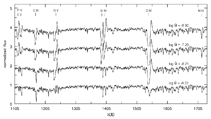
Figure 13: $\dot{M}$-sensitive lines in the far-UV and UV regions. A $vsini$ convolution of 200 km s^-1 was applied in each spectrum. Other physical parameters (e.g. $T_{eff}$ and $v_{\infty}$) are held fixed at the values derived for HD 216532 (see Table 3). The models were normalized and vertically displaced for clarity.

Table 4: Mass-loss Rates and Upper Limits Derived from Different Transitions (log units).

Star	$\dot{M}$ (C IV)	$\dot{M}$ (C III)	$\dot{M}$ (N V)	$\dot{M}$ (N IV)	$\dot{M}$ (P V)	$\dot{M}$ (Si IV)	$\dot{M}$ (Vink)
HD 216898	-9.35	$<$-7.47	$<$-8.46	$<$-7.80	$<$-7.96	$<$-7.59	-7.22
HD 326329	-9.22	$<$-7.73	$<$-8.22	$<$-7.49	$<$-7.73	$<$-7.96	-7.38
HD 66788	-8.92	$<$-7.22	$<$-8.38	$<$-7.52	$<$-7.52	$<$-7.22	-6.95
$\zeta$ Oph	-8.80	$<$-7.40	$<$-8.15	$<$-6.89	$<$-7.40	$<$-7.70	-6.89
HD 216532	-9.22	$<$-7.45	$<$-8.21	$<$-7.57	$<$-7.45	$<$-7.70	-6.92

7.1 Other $\dot{M}$ Diagnostics:

In most cases, the C iv $\lambda\lambda$1548,1551  resonance doublet is the only diagnostic available to establish mass-loss rates in late-type O8-9V stars, which brings uncertainties to the discussion of the weak wind problem. In order to overcome this situation, we have explored an alternative approach to estimate $\dot{M}$ values.

We have proceeded in the following manner: for each object of our sample, we have started with the $\dot{M}$ determined from the best fit to C iv $\lambda\lambda$1548,1551  (the final model). Then, we have gradually increased this parameter until reach the value predicted by the radiative wind theory - $\dot{M}_{Vink}$ - which for each star is a function of $T_{eff}$, mass and luminosity. We observed that as soon as we have used values higher than in our final models (yet considerably lower than $\dot{M}_{Vink}$), different wind profiles started to appear which are not observed. We have thus used this finding to establish upper limits on $\dot{M}$ from different transitions, as described below.

First, in Figure 13, we illustrate the $\dot{M}$ diagnostics found by following the procedure aforementioned. Besides C iv $\lambda\lambda$1548,1551, the lines that show significant changes are: P v $\lambda\lambda$1118,1128, C iii $\lambda 1176$, N v $\lambda$1239,1243, Si iv $\lambda\lambda$1394,1403, and N iv $\lambda$1718. When $\dot{M}$ is low (i.e. $\sim 10^{-10}$-$10^{-9}$ M_⊙ yr ^-1), N v $\lambda$1239,1243  is generally weak (or absent) and the other lines are essentially photospheric. However, when $\dot{M}$ is increased they gradually have their profiles modified and some develop a very intense P-Cygni profile when $\dot{M}_{Vink}$ is used (see for instance Si iv $\lambda\lambda$1394,1403).

The upper limits ($\dot{M}_{upper}$) for these $\dot{M}$-sensitive lines were obtained in different ways. For P v $\lambda\lambda$1118,1128, C iii $\lambda 1176$, and Si iv $\lambda\lambda$1394,1403, we have observed when the profiles started to get filled by wind emission and/or a blue absorption started to appear, deviating from the (purely photospheric) observed ones. For N v $\lambda$1239,1243, we used the strength of the whole P-Cygni profile, which generally is weak or absent in the observations. The N iv $\lambda$1718  line has a different response. Instead of getting filled in its center, an asymmetric blueward absorption profile is formed. We have then determined $\dot{M}_{upper}$ when a significant (blue) displacement from the observed feature was reached. Such peculiar behavior indicates that this line is formed in the very inner parts of the stellar wind. In the study done by Hillier et al. (2003), a similar situation is found in the homogeneous model for the O7 Iaf+ star AV 83, specially regarding S v $\lambda$1502 (see their Fig. 10).

The results obtained for each object of our sample are summarized in Table LABEL:uppermd. The C iv $\lambda\lambda$1548,1551  mass-loss rates indicated are the ones used in our best fits presented in Section 4. The predicted mass-loss rates are also shown for comparison. Below we present the models used to construct Table LABEL:uppermd and comment on each object.

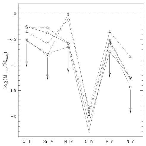
Figure 14: Mass-loss rates upper limits derived from different transitions in the ultraviolet. The stars are: HD 216898 (circled+solid line), HD 326329 (triangles+dashed line), HD 66788 (squares+dotted line), $\zeta$ Oph (asterisk+dashed-dotted line), and HD 216532 (crosses+short-long dashed line). Arrows indicate that the points represent upper limits.

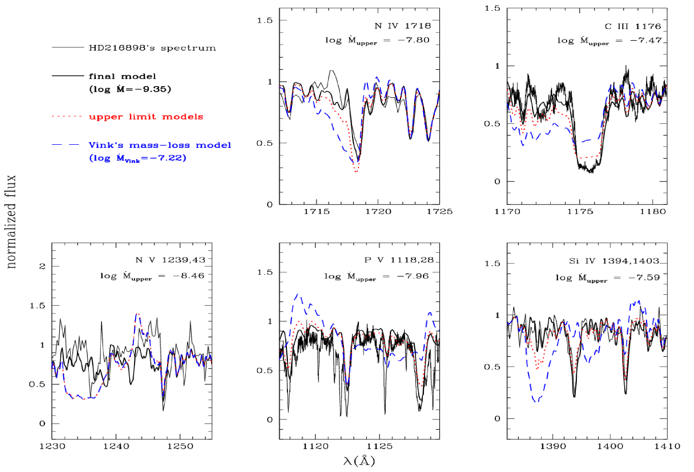
Figure 19: Upper limits for the mass-loss rate in HD 216898.

• HD 216898: In Figure 19 we show the far-UV and UV observed spectra of this object along with our final model, the models that determine the upper limits in $\dot{M}$ from each line ($\dot{M}_{upper}$; not necessarily the same in each panel), and the model with the Vink’s mass-loss rate. We can clearly note from Figure 19 that: (i) the final model presents the best fit to the observed spectra; (ii) the model with $\dot{M}_{Vink}$ presents the largest discrepancy; and (iii) the models with the upper limits for the mass-loss rate do not present satisfactory fits. This is also valid for the other objects discussed below. We note that when we have increased $\dot{M}$, the N v $\lambda$1239,1243  line quickly turned to a P-Cygni profile and remained essentially unchanged even when we have reached $\dot{M}_{Vink}$.
  

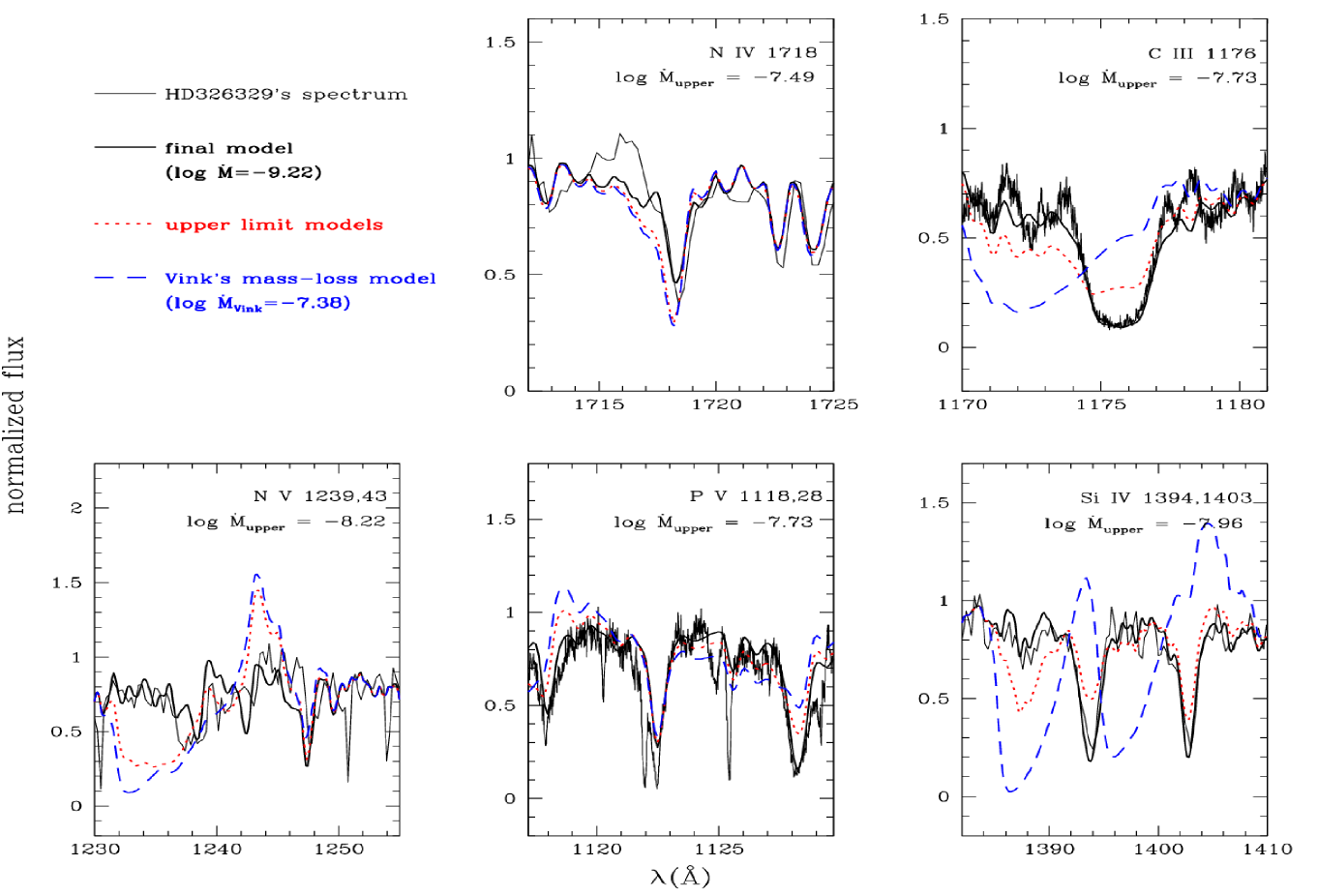
Figure 20: Upper limits for the mass-loss rate in HD326329.

• HD 326329: An analogous plot as shown for HD 216898 is presented in Figure 20 for this object. We observed that the N iv $\lambda$1718  transition is not so sensitive to $\dot{M}$ in this case. Therefore, the upper limit for $\dot{M}$ derived from this line is quite close to $\dot{M}_{Vink}$. For the other lines the situation was much clearer, i.e., the upper limits could be easily obtained.
  

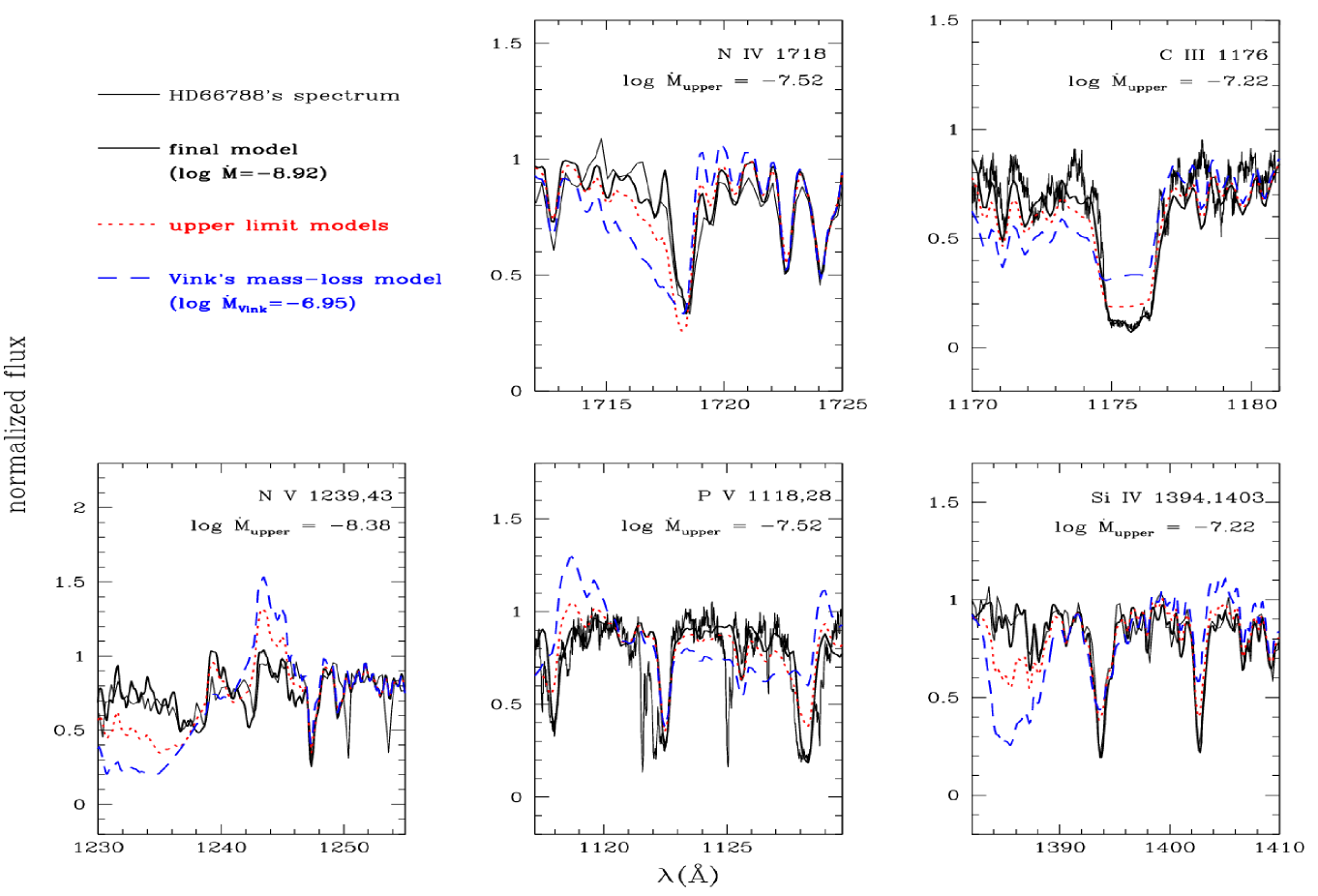
Figure 21: Upper limits for the mass-loss rate in HD66788.

• HD 66788: In Figure 21 we show the case of HD 66788. In general, the same line trends found in HD 326329 and HD 216898 are observed. We had no problems in the determination of $\dot{M}$ upper limits from each line.
  

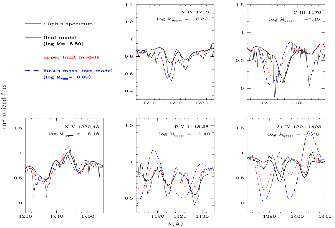
Figure 22: Upper limits for the mass-loss rate in $\zeta$ Oph.

• $\zeta$ Oph: The observed spectra and models are shown in Figure 22. Regarding N iv $\lambda$1718, we see that our final model does not present an adequate fit to the observed line, which is considerably deeper. In fact, none of the explored $\dot{M}$ values could fit this feature. By increasing the mass-loss rate however, we noted that the absorption still went blue-shifted (as in the other objects). We conservatively assume a $\dot{M}$ upper limit from this line equals to the Vink’s mass-loss. Another difficult situation is presented by N v $\lambda$1239,1243. First, unexpectedly, the model using $\dot{M}_{Vink}$ (i.e. with the strongest mass-loss rate) has a synthetic P-Cygni emission less intense than the one in the upper limit model. A slightly stronger emission is however found at $\sim$1249Å. In order to choose the upper limit model shown in the figure, we have focused in the absorption part of the P-Cygni profile. The theoretical line is deeper than observed, specially around 1235Å. We have not considered in the analysis the two (too) deep absorptions observed as part of the wind profile (see the two marks in Figure 22 in this line). These features present a large variability in $\zeta$ Oph (mainly the bluest one), which is interpreted as being due to DACs (Howarth et al. 1993; see their Figure 2). The situation for P v $\lambda\lambda$1118,1128  and Si iv $\lambda\lambda$1394,1403  is somewhat simpler. Although our final model does not present a very good match to the observed lines, it correctly predicts them in absorption. The same does not happen with the upper limit and Vink’s mass-loss models.
  

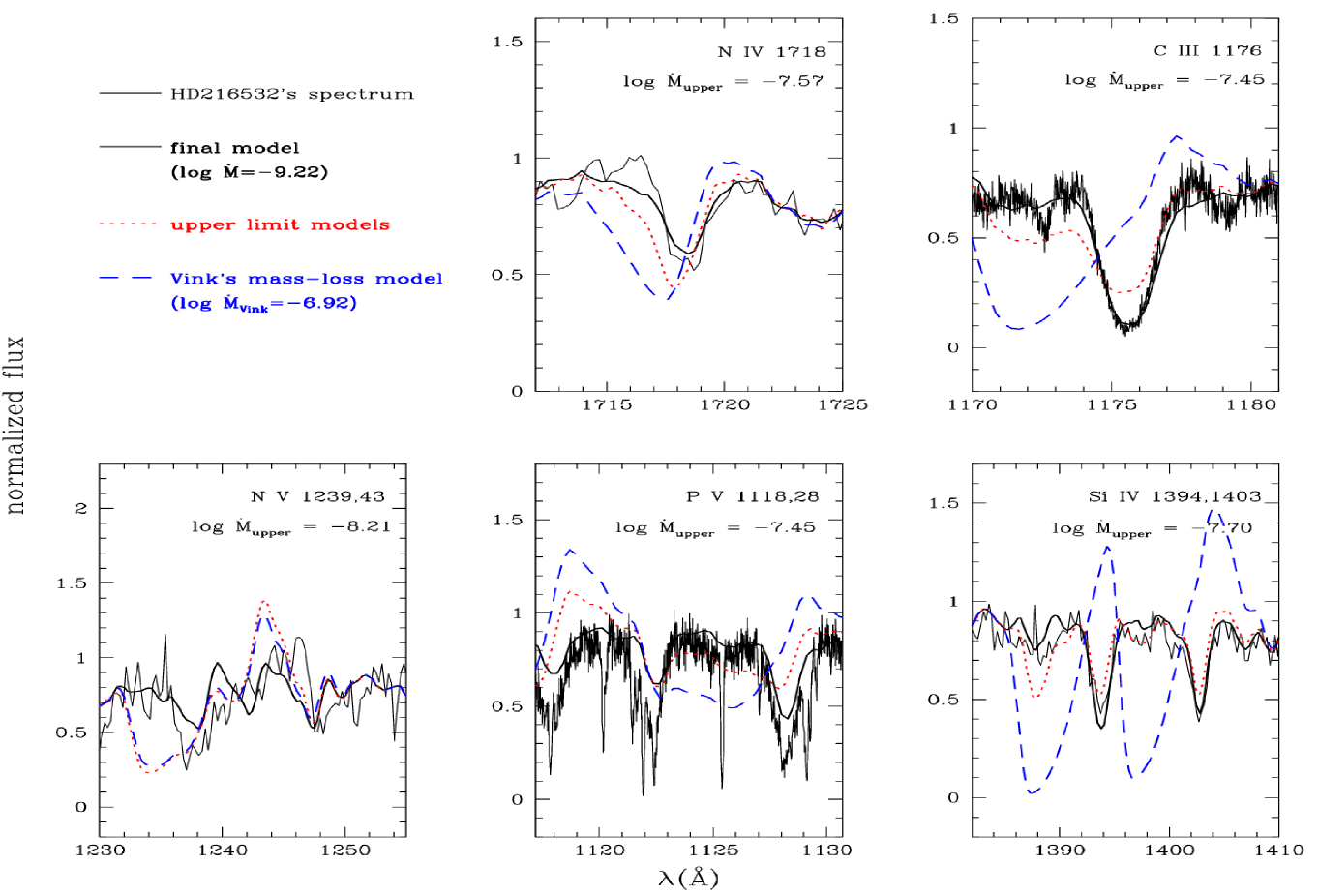
Figure 23: Upper limits for the mass-loss rate in HD 216532.

• HD 216532: In Figure 23 is shown the models and observed spectra of HD 216532. We note that the C iii $\lambda 1176$, P v $\lambda\lambda$1118,1128, and Si iv $\lambda\lambda$1394,1403  lines present a well developed P-Cygni profile with $\dot{M}_{Vink}$. Regarding the P v $\lambda\lambda$1118,1128  lines, the final model fit is not deep enough. Nevertheless, an upper limit for $\dot{M}$ can be derived without difficulty as these lines turn to emissions when $\dot{M}$ is increased, and this is not what is observed.

In Figure 14 we explore the results presented above in a graphical way. The mass-loss rates obtained are shown relative to the predicted value for each star, i.e., relative to $\dot{M}_{Vink}$. For C iv $\lambda\lambda$1548,1551, the mass-loss rates are the ones in our final models. For C iii $\lambda 1176$, Si iv $\lambda\lambda$1394,1403, N iv $\lambda$1718, P v $\lambda\lambda$1118,1128, and N v $\lambda$1239,1243, we remind that the points represent only upper limits, i.e., the mass-loss rates must be lower than what is displayed.

Strikingly, we see from Figure 14 that in all cases the points, i.e., upper limits on the mass-loss rate, fall below the theoretical line. The only exception is N iv $\lambda$1718  in the case of $\zeta$ Oph, for which we have assigned a conservative upper limit value. If we consider only the C iv $\lambda\lambda$1548,1551  and N v $\lambda$1239,1243  lines, we see that most results are below about -1.0 dex, i.e., the $\dot{M}$’s must be less than about ten times the values predicted by theory ! If we analyze all other transitions together, we see that most points fall at approximately $(-0.5\pm 0.2)$ dex. This means that the mass-loss rates are still very low: they must be less than about two to five times $\dot{M}_{Vink}$! Taken together, these results bring for the first time additional support to the reality of weak winds.

If we focus only on one object, it is also interesting to note in Figure 14 that the points below the highest point (i.e. closest to Vink’s line) have the respective theoretical lines already in disagreement with the observed ones. In this sense, whenever we skip to models/points higher than others, Figure 14 can be interpreted as errors being accumulated in the model fits.

We remind that all the models presented in this paper do not include clumping. Therefore, some of the upper limits presented above could be in fact much lower if the wind of the objects studied here are not homogeneous. In this case, we could then have that:

$$log\frac{\dot{M}_{clumped}}{\dot{M}_{Vink}}=log\frac{\dot{M}}{\dot{M}_{Vink}}+log\sqrt{f},$$

where the first term in the right-hand side is in the vertical axis shown in Figure 14. With a typical filling factor $f=0.1$, some points (depending on the wind clumping sensitivity of the respective lines) could go down, i.e. away from the Vink’s prediction, by 0.5 dex. We think however, that it is more reasonable to compare the results of homogeneous atmosphere models with radiative wind models that are also homogeneous, as it is the case in Vink et al. (2000; 2001).

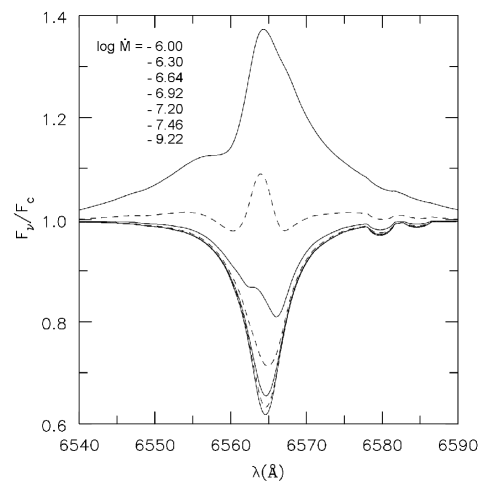
Figure 15: Sensitivity of H$\alpha$ to different values of the mass-loss rate. The model with the lowest mass-loss has log $\dot{M}=-9.22$ and it corresponds to the most intense absorption line. The model with the highest mass-loss rate has log $\dot{M}=-6.0$ and it corresponds to the most intense line in emission. The models in between are shown by alternating dashed and full lines for clarity.

7.2 H$\alpha$ behavior:

Although we have determined mass-loss rates from the far-UV and UV spectral regions, we have also analyzed the behavior of H$\alpha$ to changes in $\dot{M}$. This is an important point because as we highlighted in Section 5, the use of H$\alpha$ by Mokiem et al. (2005) seems to indicate for a few stars that there are no weak winds, i.e., the $\dot{M}$ values obtained are compatible with $\dot{M}_{Vink}$ (see also the discussion in Mokiem et al. 2007).

Previously, the work of Martins et al. (2005) had already demonstrated two things regarding this line: (i) in a low density wind ($\dot{M}\sim 10^{-9}$ M_⊙ yr^-1) the CMFGEN and FASTWIND predictions agree; (ii) for $\dot{M}$ changes from $\sim 10^{-10}$ to $10^{-9}$ M_⊙ yr^-1 the resulting CMFGEN H$\alpha$ profiles are virtually identical. Here, we extend their analysis by presenting the changes in the H$\alpha$ profile for a large range in mass-loss: from $\sim 10^{-10}$ to $10^{-6}$ M_⊙ yr^-1.

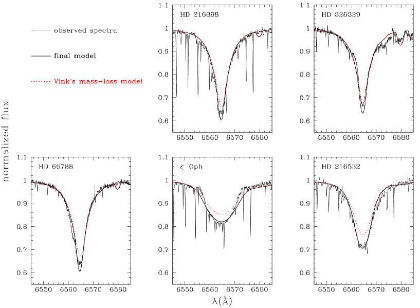
Figure 16: Fits to the observed H$\alpha$ lines in our sample using the mass-loss rates of our final models and the mass-loss rates predicted by theory ($\dot{M}_{Vink}$).

In Figure 15 we plot models with the photospheric parameters fixed and different values for the mass-loss rate. First, we note that only with a log $\dot{M}=-6.30$ the H$\alpha$ line turned to emission. For lower rates, the predictions are in absorption and therefore the measurement of $\dot{M}$ in an observed spectrum must be done based in the analysis of the wind filling of the photospheric profile. In the example shown, models with a log $\dot{M}=-9.22$, log $\dot{M}=-7.46$, log $\dot{M}=-7.20$ do not differ much. Despite a factor of one hundred in $\dot{M}$, the changes in the profiles are too small to allow a secure discrimination of a best fit model to an observed spectrum (see below). Overall, the models suggest that our confidence in mass-loss rates derived from H$\alpha$ profiles is limited to values $\gtrsim$ 10^-7 M_⊙ yr^-1. As it can be seen in Figure 15, only beyond this threshold noticeable changes start to be found.

In Figure 16 we turn our attention to the stars of our sample. The fits achieved to H$\alpha$ using our final models (i.e. with $\dot{M}$ obtained from C iv $\lambda\lambda$1548,1551) and models with $\dot{M}_{Vink}$ are presented (see Table 3 for the corresponding values). First, if we focus on HD 216898 and HD 66788, neither our final models nor the ones using $\dot{M}_{Vink}$ match the observed H$\alpha$. The models using $\dot{M}_{Vink}$ are weaker while our final models are stronger than the observed line center. However, the differences compared to the observations are very small: $\sim$0.02 of the continuum intensity. Given the uncertainties involved in the normalization of the spectra of our sample around H$\alpha$, we find very hard to choose with certainty between any of these models (and also the ones in between, i.e., with intermediate $\dot{M}$’s). As in Martins et al. (2005), we estimate that the position of the line core can have an error up to 2%. However, if a nebular contamination is likely or the signal-to-noise ratio of the spectra is not high enough, the uncertainty increases considerably. Such situations illustrate that it is not straightforward to establish $\dot{M}$ values for O8-9V stars using H$\alpha$. For HD 326329 the situation is similar, but the $\dot{M}_{Vink}$ model presents a better fit than our final model.

Interestingly, for $\zeta$ Oph and HD 216532, our final models seem to be better than the ones using $\dot{M}_{Vink}$, and not only in the line center. To use the predicted mass-loss rates for these stars thus means that we can fit neither the UV nor the optical lines! Regarding $\zeta$ Oph, Repolust et al. (2004) and Mokiem et al. (2005) have presented $\dot{M}$ measurements from H$\alpha$ based on the FASTWIND code. The former authors derived an upper limit of log $\dot{M}=-6.74$ and the latter found a mass-loss rate of log $\dot{M}=-6.85$. In both studies, the $\beta$ parameter used for the velocity law was fixed at 0.8. Although the fit in Figure 16 uses $\beta=1$, we have tested a model with the same predicted mass-loss (log $\dot{M}_{Vink}=-6.89$) and $\beta=0.8$. The synthetic H$\alpha$ line gets deeper, but it is still not enough to fit the observations. We therefore do not confirm the findings of Mokiem et al. (2005). We speculate that one reason for this can be the different data set used and their reduction. Another alternative is the existence of a discrepancy between the predicted H$\alpha$ profile by CMFGEN and FASTWIND at $\sim 10^{-7}$ M_⊙ yr^-1. This is a possibility since in the comparison made by Puls et al. (2005) we can note that these two codes can predict slightly different H$\alpha$ line intensities. In the case of an O8V or a O10V model for example (see their Fig. 17), FASTWIND tends to present a stronger H$\alpha$ absorption than CMFGEN. Such differences can affect mass-loss rate measurements for late O dwarfs obtained from this line.

8 Discussion:

It is clear from the previous section that when high mass-loss rates are used, i.e. above the values derived from C iv $\lambda\lambda$1548,1551, a considerable discrepancy is seen between the models and the observations (see Figs. 19-23). Most importantly, this is seen for lines of different ions, for each object of our sample. With these different diagnostics, the existence of weak winds gains strong additional support. Given the importance of this result, we now discuss the validity of our models.

What are the consequences if we still accept the mass-loss rates predicted by Vink et al. (2000) for late O dwarfs as the correct ones ? Given our findings, we must conclude that the expanding atmosphere models used (from CMFGEN) lack new physics or have incorrect assumptions or approximations (or both). Even with high mass-loss rates (i.e. equal or close to $\dot{M}_{Vink}$) the models should provide a reasonable fit to the observed spectra, where only a few wind lines are seen. The current wind structure/ionisation then must be changed in a drastic way for a model to predict only a weak C iv $\lambda\lambda$1548,1551  wind feature (and perhaps also a weak N v $\lambda$1239,1243), despite a high $\dot{M}$ (about one hundred times higher than the ones in this paper or even more!). One analogy that can be done is that the uppermost synthetic spectrum shown in Figure 13 would have to turn to the one essentially photospheric (bottom). Although possible, this scenario presents several difficulties.

First and foremost, contrary to the recently reported case of some B supergiants, where a few key UV wind lines could not be reproduced by CMFGEN models (see Searle et al. 2008 and also Crowther et al. 2006), we do find agreement with the observations (see Figs. 1-10). Although in most spectra only one conspicuous wind signature is observed, the lack of wind lines such as P v $\lambda\lambda$1118,1128, C iii $\lambda 1176$, Si iv $\lambda\lambda$1394,1403, and N iv $\lambda$1718, is also a constraint attained by our models. In fact, these are transitions from the photospheric region (which is smoothly connected to the wind) that can be well reproduced.

In addition, the reasonable fits that we have achieved with very low mass-loss rates would have to be merely an unfortunate coincidence. This would be also true regarding the stars analyzed by Martins et al. (2005). Another issue is that depending on the physical ingredient(s) neglected or assumptions to be revised, the theoretical hydrodynamical predictions will probably need to be re-examined. In this case, it would now mean that we should trust neither in atmosphere nor in the current radiative wind models when dealing with late O dwarf stars. The weak wind problem would then be ill-defined. Further, any future, more sophisticated models would have to achieve fits to the observed spectra similar to ours, with perhaps more free input parameters or assumptions (e.g. as in non-spherical winds).

There is no clear answer as for the missing ingredient(s) in the current atmosphere models. For massive stars in general, it is true that although CMFGEN and other codes such as FASTWIND are considered state-of-art, different physical phenomena are not taken into account properly or are not taken into account at all due to several technical challenges and lack of observational constraints (e.g. non-stationarity; wind rotation; non-sphericity; realistic description of clumping; see Hillier 2008 and references therein). It is possible that advances in some of these topics can cast a new light in the analysis of massive stars. However, the consequences regarding the weak wind problem are difficult to foresee.

In short, we believe that the inclusion of new physics or relaxation of standard assumptions certainly deserves to be addressed in future studies (with the appropriate observational constraints), but our atmosphere models for the O8-9V stars are the best working hypothesis currently available.

Below we speculate about some possibilities worth to be investigated, and thereafter present the hypothesis of highly (X-rays) ionized winds.

8.1 Magnetic fields and multi-component winds

From the best fit models, we can examine how closely the momentum absorbed by the wind matches that required to satisfy the momentum equation. In general, for the O8-9V stars, we find that the wind absorbs too much momentum. This can be illustrated by noting that the mass-loss rate from a single saturated line is approximately $L/c^{2}$ (Lucy & Solomon 1970). In all cases, this value exceeds our best fit mass-loss rates (see Table 3). While none of the wind lines in the models are saturated, there are sufficient weak lines to yield a force similar, or larger, than the single line limit.

It is unclear how this discrepancy can be removed. Possibilities include the existence of magnetic fields, and/or the presence of a significant component of hot gas. The latter could be generated by shocks in the stellar wind. As noted by Drew et al. (1994) and Martins et al. (2005), it is possible that at the densities encountered in these winds the shocked gas never cools (see also Krtička & Kubát 2009). Such gas would not be easily detectable in the UV since it could be collisionally ionized to such an extent that very few C IV and N V ions would exist. Further evidence for a significant amount of hot gas comes from the observed X-ray fluxes; the required filling factors in the models (while strongly mass-loss rate dependent) indicate that the hot gas in the wind is not a trace component.

Of interest in this regard are the distinct profiles presented by C iv $\lambda\lambda$1548,1551. While all show blue shifted absorptions, the depth and shapes differ significantly among the stars (see for instance the ones in HD 66788, HD 326329, and HD 216532). Also of concern is the general weakness of the P-Cygni emission components (with the possible exception of $\zeta$ Oph). Instead of very low mass-loss, such an absence might be related to complicated wind structures.

8.2 X-rays highly ionized winds:

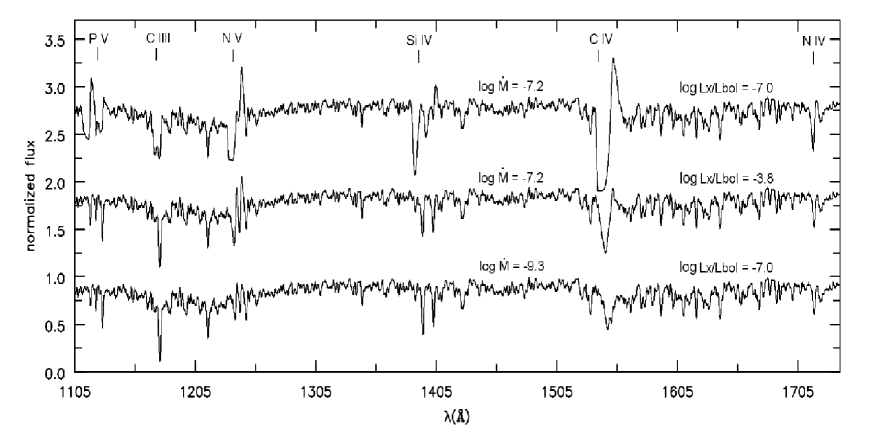
Figure 17: Effects of different log $L_{X}/L_{Bol}$ ratios in the ultraviolet synthetic spectrum. Note the similarities between the middle and bottom spectra, despite the very different mass-loss rates.

Although good fits could be achieved with very low $\dot{M}$’s, we have still studied some alternatives to have agreement with the observations using $\dot{M}_{Vink}$. It became soon clear that the most promising option was to explore high levels of X-rays emission. If most of the wind is ionized, i.e. is in the form of a hot plasma, we do not expect significant wind emission in the UV lines.

In order to test the idea above, we explored models with high values for the $L_{X}/L_{Bol}$ ratio. We have found that indeed the wind emission is decreased in the desired manner. To illustrate this, we present in Figure 17 two models with the same (typically Vink) mass-loss rate but with different values for log $L_{X}/L_{Bol}$: the canonical (-7.0) and a much higher ratio (-3.8). In addition, a third model with a very low mass-loss rate (log $\dot{M}=-9.3$; as in a typical final model) is shown with a log $L_{X}/L_{Bol}=-7.0$. Given the high level of X-rays emission, the model with a log $L_{X}/L_{Bol}=-3.8$ has most of its wind ionized and despite the high mass-loss rate, no significant line emissions take place, as in weak winds! Indeed, the synthetic spectrum with high $\dot{M}$ and log $L_{X}/L_{Bol}$ resembles the one with very low $\dot{M}$ and normal log $L_{X}/L_{Bol}$ (see the spectra in the middle and bottom of Figure 17).

In order to better quantify the result above, we have turned our attention to the ionisation fractions of P v, N v, Si iv, and C iv. For the resonance lines P v $\lambda\lambda$1118,1128, N v $\lambda$1239,1243, Si iv $\lambda\lambda$1394,1403, and C iv $\lambda\lambda$1548,1551, it is well known that what is necessary to fit their observed profiles is an appropriate value of the product of the mass-loss rate and the respective ionisation fraction - $\dot{M}\times q_{i}$ - which means to find their correct/observed optical depths (see for instance the case of P v $\lambda\lambda$1118,1128  in Fullerton et al. 2006). Thus, from our final models it can be said that we actually find:

$$\dot{M}\times q_{i}=\Psi_{i},$$ (1)

where $\Psi_{i}$ is a constant that depends on the observed spectrum and $q_{i}$ is the ionisation fraction of the ion $i$. This latter is usually defined as:

$$q_{i}=\frac{\int_{0.2}^{1}n_{i}(x)dx}{\int_{0.2}^{1}n(x)dx},$$ (2)

where $x=v(r)/v_{\infty}$ and $n_{i}$ and $n$ are the ion and element number density, respectively. We can now compute what is the ionisation fraction needed to fit the observations by using $\dot{M}_{Vink}$, which we call $q_{i,Vink}$. Since the constant $\Psi_{i}$ gives the appropriate fit to the observations, we can write:

$$q_{i,Vink}=\Psi_{i}/\dot{M}_{Vink}.$$ (3)

After we found $q_{i,Vink}$ from the equation above, for each ion, we have computed several models with the mass-loss rate fixed at $\dot{M}_{Vink}$ but with different values of log $L_{X}/L_{Bol}$. For each model, we have derived the ionisation fraction of each ion following Eqn. 2. We call these ionisation fractions $q_{X}$, i.e., the ionisation fractions for a specific log $L_{X}/L_{Bol}$ value. We have then verified which one of the several $q_{X}$ was equal to $q_{i,Vink}$, in order to find for which amount of X-rays we would have agreement with the observations using $\dot{M}_{Vink}$.

In Figure 18 we plot the ratio $q_{i,Vink}/q_{X}$ for each ion versus several log $L_{X}/L_{Bol}$ values. For simplicity, we illustrate the case of only one object of our sample, HD 216898. The first thing to note is that the ions do not behave exactly in the same manner. This is not so surprising, since they have different electronic structures and ionization potentials, and thus react differently to X-rays. If we focus on C iv and P v, we can see that only when very high log $L_{X}/L_{Bol}$ ratios are considered (around -3.0), $q_{X}$ gets close to $q_{i,Vink}$. Otherwise, their ratio is much lower than unity. In the case of Si iv, $q_{i,Vink}/q_{X}$ remains very small regardless the value of log $L_{X}/L_{Bol}$. However, an increase is observed when we use a log $L_{X}/L_{Bol}$ near -3.0. For a log $L_{X}/L_{Bol}\sim-7$ for example, we have $q_{i,Vink}/q_{X}\sim 5\times 10^{-5}$. For log $L_{X}/L_{Bol}\sim-3$, this ratio is much higher, $q_{i,Vink}/q_{X}\sim 0.005$. For this ion therefore, the conclusion is that even more X-rays seems to be required to $q_{X}$ reach $q_{i,Vink}$. The situation for N v is quite interesting: for both low and high values of log $L_{X}/L_{Bol}$, the $q_{X}$ approaches $q_{i,Vink}$. This is however, not hard to explain. For high values of log $L_{X}/L_{Bol}$, we observed that practically all nitrogen is concentrated in N vi. Thus, the ionisation fraction $q_{X}$ obtained for N v is low as the ionisation fraction of Vink, $q_{Vink}$, computed from Eqn. 3. On the other hand, when very low log $L_{X}/L_{Bol}$ ratios are considered, we verified that most of the nitrogen is in N iii-iv. Thus, again, a very low $q_{X}$ is obtained for N v. In practice, this means that the observed, weak N v $\lambda$1239,1243  line (or its absence!), can be reproduced by models using $\dot{M}_{Vink}$ with either very low or large amounts of X-rays.

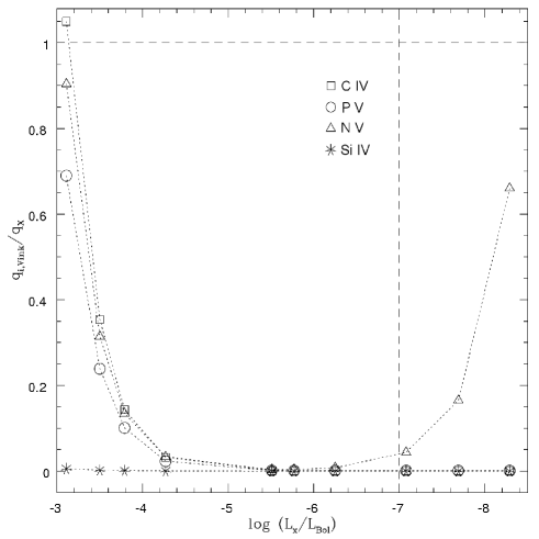
Figure 18: Ionisation fractions as a function of log $L_{X}/L_{Bol}$. The values for $q_{X}$ were computed using Eqn. 2 and $\dot{M}_{Vink}$. The $q_{i,Vink}$ values were derived from Eqn. 3 (see text for more details).

Our conclusion from both Figures 17 and 18 is that the only way to have high mass-loss rates ($\dot{M}_{Vink}$) and still agree with the observed spectra is by using a log $L_{X}/L_{Bol}\gtrsim-3.5$. Unfortunately, this is not supported by X-rays observations, where the log $L_{X}/L_{Bol}$ values measured are normally about -7.0 (see e.g. Sana et al. 2006) with a scatter of about $\pm 1.0$. It is encouraging however, to explore in future studies different scenarios of X-rays emission in stellar winds.

9 Conclusions:

We have analyzed a sample of five late-type Galactic O dwarfs by using atmosphere models from the CMFGEN and TLUSTY codes (HD 216898, HD 326329, HD 66788, $\zeta$ Oph, and HD 216532). Model fits for the far-UV, UV and optical observed spectra were presented, from which stellar and wind parameters were obtained. The mass-loss rates were obtained first using the C iv $\lambda\lambda$1548,1551  feature and then we have explored new diagnostic lines. Our main motivation to study O8-9V stars was to address the so-called weak wind problem, recently introduced in the literature. The main findings of our study are summarized below:

• The stellar parameters obtained for our sample are quite homogeneous (see Table 3). Surface gravities of about 3.8 (after correcting for $vsini$) to 4.0 and $T_{eff}$’s of 30 to 34$kK$ were obtained. These values show a good agreement with the latest calibrations of Galactic O star parameters, regarding the spectral types of the programme stars.
  

• By using the C iv $\lambda\lambda$1548,1551  line we have derived mass-loss rates considerably lower than theoretical predictions (Vink et al. 2000). A discrepancy of roughly two orders of magnitude is observed (see Figure 11). We thus confirm the results of the study of Martins et al. (2005) of weak winds among Galactic O8-9 dwarf stars. We also confirm a breakdown or a steepening of the modified wind momentum luminosity relation for low luminosity objects (log $L_{\star}/L_{\odot}\lesssim 5.2$).
  

• We have investigated the carbon abundance based on a set of UV (C iii $\lambda 1176$) and optical photospheric lines. We estimated that the following range is reasonable for our programme stars: $0.5\lesssim\epsilon_{C}/\epsilon_{C_{\odot}}\lesssim 2$ (in mass fractions). Although the uncertainty is large, it is not large enough to be the reason of the weak wind problem.
  

• We have explored different ways (besides using C iv $\lambda\lambda$1548,1551) to determine mass-loss rates for late O dwarfs. We have found that P v $\lambda\lambda$1118,1128, C iii $\lambda 1176$, N v $\lambda$1239,1243, Si iv $\lambda\lambda$1394,1403, and N iv $\lambda$1718  lines are good diagnostic tools. We have used each of them to derive independent mass-loss rate limits, for each star of our sample. We have found that together with C iv $\lambda\lambda$1548,1551, the use of the N v $\lambda$1239,1243  line implies in the lowest $\dot{M}$ upper limit rates. The results obtained show that the $\dot{M}$ values must be less than about -1.0 dex compared to $\dot{M}_{Vink}$. By considering the other lines, we still find very low mass-loss rates. The results obtained show that $\dot{M}$ must be less than about $(-0.5\pm 0.2)$ dex compared to $\dot{M}_{Vink}$. They bring additional support to the reality of weak winds.
  

• Upper mass-loss rate limits derived from N iv $\lambda$1718  and C iii $\lambda 1176$  can be a factor of three, or more, lower than the theoretical mass-loss rates of Vink. This is crucial in confirming a mass-loss discrepancy as N iv $\lambda$1718  and to a lesser extent C iii $\lambda 1176$  are formed close to the photosphere, where the uncertainties in the ionization structure should be much less than in the (outer) wind.
  

• We have analyzed the H$\alpha$ line and we observed that its profile is insensitive to $\dot{M}$ changes when we are in the $<10^{-8}$M_⊙ yr^-1 regime. For some objects of our sample it is uncertain to choose between the H$\alpha$ fit presented by our final models and the ones using $\dot{M}_{Vink}$. The interpretation of the results is hindered by uncertainties in the continuum normalization of echelle spectra. Such situation gets even more complicated if a contamination by nebular emission is likely. For the stars HD 216532 and $\zeta$ Oph, the fits to the observed H$\alpha$ lines using $\dot{M}_{Vink}$ were not satisfactory. This result shows that even when H$\alpha$ is used, lower than predicted mass-loss rates can be preferred.
  

• We have investigated ways to have agreement with the observed spectra of the O8-9V stars using the mass-loss rates predicted by theory ($\dot{M}_{Vink}$). The only mechanism plausible that we found is X-rays. By using high values for the log $L_{X}/L_{Bol}$ ratio, we could observe that very few wind emissions takes place, as in models with very low mass-loss rates ($\sim 10^{-10}-10^{-9}$ M_⊙ yr^-1). However, the values needed to be used (log $L_{X}/L_{Bol}\gtrsim-3.5$) are not supported by the observations, which usually measure log $L_{X}/L_{Bol}$ values near -7.0.

Although our analysis was performed with state-of-art atmosphere models, there are a couple of issues which still need to be addressed in future studies. For example, some stars of our sample (HD 326329 and HD 216532) present a deep C iv $\lambda\lambda$1548,1551  feature that could not be well reproduced. The origin of this extra absorption remains to be investigated (see Section 8.1). Studies concerning non-spherical winds, specially for stars that are fast rotators, are also of great interest. First synthetic spectra computed by our group have shown interesting line profile changes. A deeper analysis is needed to see if some of the discrepancies found in the case of $\zeta$ Oph can be solved. Furthermore, a more realistic treatment or even alternative descriptions of the X-rays emission in the atmosphere models (e.g. in conformity with the magnetic confinement scenario; Ud-Doula & Owocki 2002) could bring valuable informations. First steps in this direction have been taken by Zsargó et al. (2009). As we have shown in Section 8.2, X-rays are an efficient mechanism to change the ionisation structure of the stellar winds.

It would be also very useful to analyze a sample of O stars having log $L_{\star}/L_{\odot}$ near $\sim 5.2$. The disagreement between atmosphere models and theoretical predictions for Galactic stars seems to start around this value. The candidate spectral types would be O6.5V, O7V, and O7.5V. Also, this same question needs to be better studied in metal-poor environments, i.e. in the LMC and SMC. We intend to investigate these issues in a future paper.

From the point of view of the hydrodynamics, there are also important questions that could be addressed. In the work of Vink et al. (1999; 2000; 2001), a predicted mass-loss rate is computed based on a set of ISA-WIND models (de Koter et al. 1997) plus the use of a Monte-Carlo technique to compute the radiative acceleration ($g_{L}$). Although the results obtained by their procedure are self-consistent, it should be kept in mind that the ISA-WIND atmosphere models do not include the effect of X-rays. As the wind ionization can be changed significantly, new radiative accelerations can be found and perhaps new predicted mass-loss rates might be derived. Within this picture, the agreement with the Vink et al. predictions for early O dwarfs may be understood, since their winds are not seriously affected by X-rays.

Our results bring new constraints to the weak wind problem. Galactic O8-9V stars seem to present very low mass-loss rates, as indicated by the C iv $\lambda\lambda$1548,1551  feature, and also additional spectral diagnostics. The existence of weak winds poses a challenge to the current radiative wind models, and possibly has important consequences to the massive stellar evolution theory.

Appendix A $\dot{M}$ upper limits:

In this Section, we present the model fits used to establish upper limits on the mass-loss rate from different UV lines.