A Short Foucault Pendulum Free of Ellipsoidal Precession

Abstract

A quantitative method is presented for stopping the intrinsic precession of a spherical pendulum due to ellipsoidal motion. Removing this unwanted precession renders the Foucault precession due to the turning of the Earth readily observable. The method is insensitive to the size and direction of the perturbative forces leading to ellipsoidal motion. We demonstrate that a short (three meter) pendulum can be pushed in a controlled way to make the Foucault precession dominant. The method makes room-height or table-top Foucault pendula more accurate and practical to build.

I Introduction

Léon Foucault built his first pendulum to demonstrate the turning of the Earth in the basement of a building, using a roughly two meter long fiber fou . He also soon recognized the problem arising from the intrinsic precession of a spherical pendulum caused by unwanted ellipsoidal motion. Imperfections in the suspension or initial conditions of the pendulum generally cause this to quickly grow to the point that the precession due to the Earth’s turning is overwhelmed. The pendulum can come to precess in either sense (clockwise or counterclockwise) at almost any rate, or indeed even cease all precession. These practical problems are mitigated in pendula of great length, and so most are constructed to have lengths of tens of meters, starting with the celebrated 67 m long device built by Foucault in Paris in 1851.

The precession of an ideal spherical pendulum with no ellipsoidal motion is caused by the non-inertial nature of the reference frame tied to the surface of the Earth. The so-called Coriolis force advances the plane of the pendulum’s motion by an amount

$$\Omega_{F}=\Omega_{Earth}\sin\theta_{latitude}$$ (1)

where $\Omega_{Earth}$ is the sidereal rate of rotation of the Earth, $\theta_{latitude}$ is the latitude of the pendulum measured from the equator, and $\Omega_{F}$ is the Foucault precession rate; many textbooks treat this problem. Near $40^{o}$ northern latitude, this amounts to almost $10^{o}$ of clockwise advance per hour, for an 18 hour half-rotation of the pendulum, after which the motion repeats. This amount of precession is easily masked, however, by the intrinsic precession of a less than perfect pendulum that develops some non-planar ellipsoidal motion.

The construction of a room-height or table-top version of a Foucault pendulum thus presents a technical challenge, first to minimize the amount of ellipsoidal motion that accrues as the pendulum swings, and secondly to compensate in some way for the irreducible amount of this motion that remains. In this paper we will first discuss the dynamics of the spherical pendulum that lead to the problem (Section II). Then we introduce a method that stops the ellipsoidal motion of the pendulum from causing precession, and show that this immunity is, to first order, independent of the minor axis of the ellipse. The method hinges on the observation that pushing the pendulum bob away from the origin after it passes, rather than either pulling it in or alternately pulling and pushing it, acts in a way to counter the unwanted intrinsic precession (Section III). We then present the design of a pendulum and a driving mechanism to exploit this method (Section IV), and demonstrate the validity of this approach by discussing the supporting experimental results (Section V). Finally, we contrast our results with earlier published work on Foucault pendula and summarize how our method and design are new and unique (Section VI).

II The Problem of Intrinsic Precession

The dynamics of the idealized spherical pendulum are determined by the centrally-directed force of gravity and initial conditions, and lead to approximately elliptical motion with a semi-major axis a and a semi-minor axis b, as shown in Fig. 1. It is somewhat counter-intuitive but true that the centrally-directed restoring force of gravity results in a constant intrinsic precession rate $\Omega$ about the z axis. This precession arises from the symmetry-breaking condition of having a finite minor axis, b. The rate is linearly proportional to b, and its sense is in the same direction as the ellipsoidal motion. An example of the exact path of a pendulum with a large ratio of b/a is given in Fig. 2, which illustrates a numerical solution of the equations of motion of a spherical pendulum.

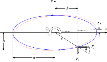
Figure 1: Planar view of the approximate path of a spherical pendulum with semi-major axis a and semi-minor axis b that is moving in a counterclockwise ellipsoid. The suspension is centered on the z axis above the origin. The pendulum is precessing at rate $\Omega$, and in one full cycle the apex advances by a distance $\Delta y$, as suggested by the light dotted and rotated ellipse. The impulsive driving force is applied at x = d, and it is resolved into components parallel and perpendicular to the major axis. The minor axis can be larger or smaller, resulting in a b-dependent magnitude of the transverse force $F_{\bot}$ for a fixed longitudinal force $F_{\parallel}$.

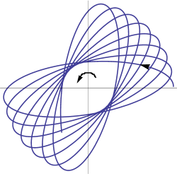
Figure 2: Numerical simulation (using Mathematica) of a spherical pendulum with a large ratio of semi-minor to semi-major ellipse axes. The arrows indicate the counterclockwise intrinsic precession, in the same sense as the motion of the pendulum.

Any ellipsoidal motion that develops in a pendulum will result in an intrinsic precession rate $\Omega$ that is wholly unrelated to the Foucault precession $\Omega_{F}$ of Eq (1). This has been worked out in detail by Olsson ols1 ; ols2 and Pippard pip , among others, and it appears in some textbooks, for example in Ref syn . The main result is

$$\Omega=\frac{3}{8}\omega_{0}\frac{ab}{L^{2}},$$ (2)

where $\omega_{0}=2\pi/T=\sqrt{g/L}$ is the pendulum’s angular frequency, L is the length, T is the period, and g is the acceleration due to gravity. The formula is the lowest-order term in a complicated motion, but it is easily sufficient for our purpose. The area of an ellipse, A, is given by $A=\pi ab$, so another way to write the intrinsic precession rate is

$$\Omega=\frac{3}{4}\frac{A}{L^{2}T}.$$ (3)

From the first expression, note that the ratio of $\Omega$ (the very slow intrinsic precession) to $\omega_{0}$ (the rapid pendular rate) is proportional to the ratio of the area of the ellipse to the area of a sphere of radius L, that is,

$$\frac{\Omega}{\omega_{0}}=\frac{3}{2}\frac{\left(\pi ab\right)}{\left(4\pi L^{2}\right)}.$$ (4)

To minimize this ratio, Foucault pendula are generally made with L very large compared to the axes a and b, since it is comparatively easy to keep b small while making L large.

Besides causing precession, ellipsoidal motion changes the central oscillation frequency of the pendulum from $\omega_{0}$ to

$$\omega=\omega_{0}\left(1-\frac{1}{16}\frac{a^{2}+b^{2}}{L^{2}}\right).$$ (5)

The fractional change in frequency due to a finite semi-minor axis b turns out to be of order $10^{-7}$, and therefore negligible for the present discussion.

Every Foucault pendulum, no matter how carefully constructed to avoid asymmetries in its suspension, and no matter how carefully “launched” to make ellipsoidal area A as small as reasonably achievable will, over time, acquire an intrinsic precession $\Omega$ that can easily grow to overwhelm the Coriolis-force induced Foucault precession $\Omega_{F}$. Near $40^{o}$ latitude, for a pendulum of length L = 3.0 meters and semi-major axis a = 16. cm, the Foucault rate is equaled with a semi-minor axis of b = 3.9 mm. The unwanted intrinsic precession may add or subtract from the Foucault precession; when it is subtractive, then the pendulum stops all precession when the corresponding value of b is reached. In our experience, it is easy to launch such a pendulum with semi-minor axis well under one millimeter, but under free oscillation, on the time scale of only two to three minutes, b grows enough such that $\Omega$ dominates $\Omega_{F}$.

When the pendulum at an extremum, at $x=\pm a$ in Fig. 1, its motion is entirely transverse, with momentum $m\dot{y}$ as large as it gets. Preferential damping of this component of the motion will reduce the unwanted ellipsoidal excursions. In previous work, this has been tried using a so-called Charron’s ring around the suspension wire near the top cha1 ; cha2 , or letting a part of the pendulum bob scrape an annular disk cra1 ; cra2 at r = a, or using eddy current damping between a permanent magnet in the bob and a non-ferrous metal annular disk mas located near x = a. We adopt the touch-free eddy-current damping method in the design we present later in this paper. Even in principle, none of these methods will stop ellipsoidal motion completely, so an additional method is needed to cope with any remaining intrinsic precession.

Every pendulum suffers dissipative losses of energy, mainly due to air friction. Long, very massive, museum-type pendula can simply be relaunched once every day or so, but a small pendulum has a free exponential decay time of order one half hour, so a “driving” mechanism is needed to restore the lost energy. Various mechanisms have been reported for this task cra1 ; cra2 ; pri ; mas . Like some others, we will use magnetic induction to sense the passage near the origin of a permanent magnet embedded in the pendulum bob. A carefully-timed electromagnetic impulse then imparts lost momentum to the bob. We will introduce a quantitative method for using a magnetic push not only to compensate for dissipative losses, but also to compensate for ellipsoidal precession.

The perturbations that lead to ellipsoidal motion are, in our experience, in approximate decreasing order of severity, (1) internal stresses or other imperfections in the fiber supporting the pendulum bob, (2) less than perfectly symmetric suspension of the fiber at its upper end, (3) nearby iron objects that result in asymmetric force on the drive magnet in the bob, (4) a driving coil that is not sufficiently level and centered under the pendulum. All but the first of these were straightforward to reduce to insignificance, but the first was persistent. This led to the necessity of finding a method to evade the problem of ellipsoidal motion rather than to remove it. There is no simple force law that leads to the intrinsic precession $\Omega$, but rather it is an inescapable feature of the spherical pendulum. Nevertheless, we can apply a separate perturbative force to counteract, i.e. nullify, the intrinsic precession. We discuss this in the next section.

III Method to Nullify Intrinsic Precession

As shown in Fig. 1, the driving force that pushes the pendulum away from the origin can be thought of as consisting of components parallel and perpendicular to the major axis. The parallel component $F_{\parallel}$ is the larger one, and it is adjusted to overcome the dissipative forces such as air resistance. The perpendicular component of the pushing force $F_{\bot}$ counteracts the intrinsic precession, and we will now show that it is possible to select distance d at which the impulsive drive force is applied to stop the precession $\Omega$. The crucial result will be that this distance is independent of semi-minor axis b. Starting from $x=-a$, in one half cycle of duration ${T\mathord{\left/{\vphantom{T2}}\right.\kern-1.2pt}2}$, intrinsic precession advances the ellipse in angle by ${\Omega T\mathord{\left/{\vphantom{\Omega T2}}\right.\kern-1.2pt}2}$. The pendulum arrives at $x\simeq+a$ and

$$y\equiv\Delta y=\frac{1}{2}a\,\Omega T,$$ (6)

where $\Delta y$ is the transverse displacement at the apex of the ellipse. However, we arrange to apply an impulsive momentum change at $x=d$ that is calibrated to move the pendulum bob by a distance $-\Delta y$ as it traverses the remaining longitudinal distance $a-d$. If this is done, the bob will arrive at location $x=a$, $y=0$, as desired. The impulse and momentum change are related by

$$m\,\Delta v_{y}=F_{\bot}\Delta t,$$ (7)

where $\Delta t$ is the duration of the applied force and m is the mass of the bob. It turns out that $\Delta t$ is a few milliseconds, compared to hundreds of milliseconds for the duration of the swing, so it is appropriate to use the impulse formulation of Newton’s second law. We treat this perturbation in the y direction as though the bob were free of other forces, which is reasonable since $\Delta y$ is of order 10 microns compared to a of order 10 centimeters. The horizontal component of the motion is simply

$$x(t)=a\sin\omega_{0}t,$$ (8)

where $\omega_{0}$ is the angular frequency characterizing the pendular oscillations. To good accuracy, the time $t_{d}$ between passage closest to the origin and the instant the pendulum reaches x = d is thus

$$t_{d}=\frac{1}{\omega_{0}}\sin^{-1}\frac{d}{a}.$$ (9)

In one quarter of the full period T the pendulum reaches its apex. Therefore, one way to write a relation between the distance $\Delta y$ that the pendulum advances and the transverse velocity $\Delta v_{y}$ that must be imparted by the driver is

$$\Delta y=\Delta v_{y}\left(\frac{1}{4}T-t_{d}\right) =\frac{\Delta v_{y}}{\omega_{0}}\left(\frac{\pi}{2}-\sin^{-1}\frac{d}{a}\right)$$

$$=\frac{\Delta v_{y}}{\omega_{0}}\cos^{-1}\frac{d}{a}.$$ (10)

From the geometry of the situation shown in Fig. 1 we see that that the driving force components are related by

$$\tan\theta=\frac{y}{d}=\frac{F_{\bot}}{F_{\parallel}},$$ (11)

and, using the formula for an ellipse

$$\left(x/a\right)^{2}+\left(y/b\right)^{2}=1,$$ (12)

we have

$$F_{\bot}=F_{\parallel}\frac{b}{d}\sqrt{1-\left(\frac{d}{a}\right)^{2}}.$$ (13)

Combining Eqs (III), (7), (13), (6), and (2) we arrive at

$$\Delta y =\frac{1}{2}a\left(\frac{3}{8}\omega_{0}\frac{ab}{L^{2}}\right)\left(\frac{2\pi}{\omega_{0}}\right)$$

$$=\frac{F_{\parallel}\Delta t}{m\omega_{0}}\frac{b}{d}\sqrt{1-\left(\frac{d}{a}\right)^{2}}\cos^{-1}\frac{d}{a}.$$ (14)

One sees in Eq (III) the crucial cancellation of the factor b that occurs between the intrinsic precession rate and in the perpendicular component of the force. This leads to the result that follows being independent of the transverse size of the ellipse. This, in turn, means the result is insensitive to exactly what non-central forces may act on the pendulum to cause non-vanishing ellipsoidal motion. An approximation is being made that $F_{\parallel}$ does not depend on b; this will be justified later.

It is now convenient to introduce some dimensionless scaling parameters. Let

$$Q\equiv\frac{\pi}{2}\frac{ma\omega_{0}}{F_{\parallel}\Delta t},$$ (15)

which is the ratio of the momentum of the pendulum as it crosses the origin to the momentum kick it receives on each half oscillation. The denominator is the momentum the driver must supply to compensate for the dissipative losses in order to maintain the full amplitude of the swing. The factor of $\pi/2$ stems from letting Q represent the conventional “quality factor” of an oscillator, specifically that

$$Q=2\pi\frac{{\rm Total\;Energy}}{{\rm Energy\;Loss\;per\;Cycle}}.$$ (16)

We expect this ratio to be quite large, on the order of 1000. Then let

$$\alpha=\frac{a}{L}$$ (17)

be the scaled amplitude of the pendulum, that is, the amplitude divided by the length; this parameter is of order 0.1 for a practical pendulum. Next, let

$$\delta=\frac{d}{a}$$ (18)

be the scaled distance from the origin at which the driving force is applied, written as a fraction of the amplitude; this value can range from near zero to unity. With these dimensionless variables, Eq (III) can be written

$$\boxed{\frac{3}{4}Q\alpha^{2}=\frac{\sqrt{1-\delta^{2}}}{\delta}\cos^{-1}\delta}$$ (19)

Equation (19) is the main result of this model. It relates the scaled distance $\delta$ at which the impulsive driving force must be applied on each half oscillation, to the physical parameters of the pendulum, specifically the scaled amplitude $\alpha$ and the quality of the oscillator Q. When Eq (19) is satisfied, the intrinsic precession is stopped or nullified, and the result is independent of the transverse size of the ellipse. Figure 3a is an illustration of this result for the cases of three different lengths of pendulum, each with a maximum excursion of 0.15 meters, as a function of the oscillation parameter, Q. It is seen that a low-loss pendulum with a larger value of Q will have to be pushed when it is closer to the origin, while a pendulum with more dissipative losses, and therefore lower Q, will have be driven further away from the origin. A high-quality, low-loss pendulum needs little energy input. Therefore, the transverse kick, which scales in magnitude with the longitudinal kick at a given $\delta$, must be applied early in the ellipsoidal swing, when the force has a larger transverse component. Part (b) of Fig. 3 illustrates the relationship between the location of the impulse, $\delta$, and the time, $t_{d}$, at which it is applied, as per Eq (9).

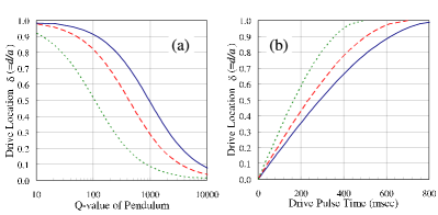
Figure 3: (a) For three pendulum lengths (L) with amplitude of 0.15 meter, the relationship of the scaled driving distance ($\delta=d/a$) versus the quality factor Q for the oscillation. Curves are for an L = 3.0 meter (solid blue), 2.0 meter (dashed red) and 1.0 meter pendulum (dotted green). (b) For the same pendulum lengths as in (a), the distance versus time relationship for the driving pulse.

Taken together, the two parts of the Fig. 3 enable design of a Foucault pendulum not plagued by intrinsic precession. For example, a 3.0 meter long pendulum with a 0.15 meter amplitude ($\alpha=0.050$) and a quality factor of $Q=1000$ must receive its impulsive drive at $\delta=.49$, which corresponds to time $t_{d}=284$ msec and a drive location of d = 7.4 cm from the origin. On the other hand, a 1.0 meter long pendulum with the same $\alpha$ and Q must receive its drive pulse at $\delta=.088$, at a time of 28 msec and 1.3 cm from the origin.

As introduced in Eq (15), Q is proportional to the ratio of the momentum of free oscillation at the origin to the damping/driving momentum that accrues with each half period of oscillation. In fact, it is quite easy to measure this parameter for an actual pendulum by measuring the period, T, and the exponential decay time, $\tau$. The motion of the pendulum in the presence of velocity-dependent losses such as air friction is given, to a good approximation at low speeds, by the damped harmonic oscillator formula

$$x(t)=ae^{-t/\tau}\sin\omega_{0}t.$$ (20)

The momentum loss between times t = 0 and t = T/2 is

$$m\dot{x}(0)-m\dot{x}(T/2)=ma\omega_{0}(1-e^{-T/2\tau})\cong ma\omega_{0}\frac{T}{2\tau}.$$ (21)

This leads to

$$Q=\pi\frac{\tau}{T},$$ (22)

from which Q can be determined experimentally. For the actual three meter pendulum discussed below, we found the decay time to be about 30 minutes and hence Q to be roughly 1600. Eq (22) can be used with Eq (19) in order to express Eq (19) in dimensioned variables as

$$\frac{3}{8}\sqrt{\frac{g}{L}}\left(\frac{a}{L}\right)^{2}\tau=\frac{\sqrt{a^{2}-d^{2}}}{d}\cos^{-1}\left({d\mathord{\left/{\vphantom{da}}\right.\kern-1.2pt}a}\right).$$ (23)

One important approximation that was made needs to be examined. In going from Eq (III) to Eq (19), the cancellation of the semi-minor ellipse parameter b was crucial to showing that the result is independent of inevitable changes in the size of the pendulum’s ellipsoidal motion. In fact, $F_{\parallel}$ does depend very slightly on b in the design we will discuss in the following sections. The pushing agent is a magnetic coil that produces a pulsed dipole field. It acts against a permanent magnetic dipole inside the pendulum bob. Though we operate in the near field of the coil, we presume that the magnetic field has a distance dependence of the dipole form $B(r)=B_{0}(r_{0}/r)^{3}$, where $B_{0}$ and $r_{0}$ are suitable scales. The dipole-dipole repulsion that drives the pendulum goes as the gradient of this field, so the interaction has the form

$$\vec{F}=\vec{F}_{0}(r_{0}/r)^{4},$$ (24)

where the components of $\vec{F}$ are what we earlier called $F_{\bot}$ and $F_{\parallel}$. It is easy to expand this expression to show that

$$F_{\parallel}=F_{0}\left(\frac{r_{0}}{d}\right)^{4}\left\{1-\frac{5}{2}\left(\frac{b}{d}\right)^{2}\left(1-\delta^{2}\right)\right\}.$$ (25)

As seen in the second term in the curly brackets, there is a quadratic dependence on the semi-minor axis b that we ignored earlier. This term is very small: for typical values of $\delta=d/a\simeq 6.0cm/16.0cm=0.375$, and $b/d\simeq 0.5cm/6.0cm=0.083$, the second term is 0.015, which is much less than 1.0. Hence this approximation was justified.

IV Experimental Setup

To verify the mathematical model discussed above, a pendulum of about three meter length was built. The mechanics and drive electronics will be described here. An image of the lower end of the setup is shown in Fig. 4.

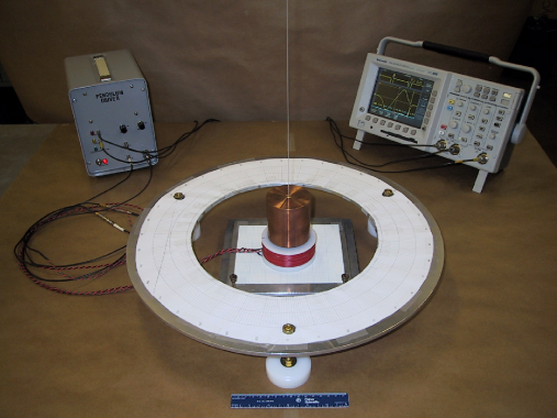
Figure 4: Image of the copper pendulum bob suspended above the sensing and driving coils (red wire on a white bobbin). The aluminum damping ring on brass legs is seen. The white band carries angular position markings. The driver box and an oscilloscope are visible in the background.

The mass of the pendulum was in the form of a lathe-turned copper cylinder, with a diameter of 2.75” (6.99 cm) and height 3.00” (7.62 cm). A 3/8” (.953 cm) axial hole was drilled and tapped to accept a small threaded set screw with a 0.040” (0.10 cm) hole in its center. The small hole was for the fiber suspending the pendulum, and the threading was used to adjust the distance between the center of mass and the suspension point. In practice, the fiber was held flush with the top surface of the bob. The bottom of the cylindrical bob was chamfered by 0.10” (0.25 cm) to allow closer approach to the damping ring. To hold the permanent magnet, a recess was milled into the bottom of the mass, of diameter 3/4” (1.90 cm) and depth 1/4” (0.635 cm), which were the dimensions of the magnet. The total mass of the pendulum bob, apart from the magnet, was 2.47 kg. This is a small mass compared to what has generally been reported for Foucault pendula.

The fiber suspending the mass was an ordinary and inexpensive polymer material of the type used for yard trimmers. The diameter was 0.040” (0.10 cm). The cross section of the fiber was circular and the diameter was uniform to better than 1%. The polymeric material was thought to be advantageous due to its lack of crystalline internal structure. It was found that the polymer material was very flexible, yet strong, and did not suffer the bending fatigue and eventual failure of some metal fibers we tried. In practice, we found that the growth of elliptical motion of the pendulum was dominated by an unobservable non-uniformity of this fiber, but it was less severe than with various metal fibers. Tests wherein the fiber was rotated without changing any other aspect of the pendulum showed this to be the case. Thermal expansion and contraction of the fiber was large enough to necessitate occasional shimming of the pendulum’s length at the level of about one millimeter.

The upper end of the fiber passed through a close-fitting drilled hole in an aluminum plate. The hole had a sharp rim, and no special steps were taken to soften the bend of the fiber as it exited the hole. On the upper side of the plate the fiber was clamped in a way that thin shims could be inserted to fine tune the length. The plate was leveled and clamped to rigid brackets on the ceiling of the laboratory. The upper support of the fiber used in this setup, though carefully arranged, was certainly less exacting than what has been found to be necessary for other Foucault pendula reported in the literature. We view this as an advantage of our design.

The permanent magnet placed inside the pendulum bob was a neodymium-iron-boron disk magnet, placed with its dipole axis vertical. The axial field strength was 2.1 kGauss on contact, but it varied by $\pm$10% from one edge of the disk to the other. Similarly, the radial field was 1.0 kG at the edge of the disk, but varied also by $\pm$10% from one side to the other. Surprisingly perhaps, these variations did not affect the performance of the pendulum.

One purpose of the magnet was to provide eddy-current damping when the bob passed over an aluminum ring near the extrema of its motion. This “damping ring” had an inner diameter of 11 7/8” (30 cm), and was 1/4” (0.64 cm) thick. Three legs made of threaded brass rod were used to level the ring to a precision of less than half a millimeter of variation around the perimeter. The amplitude of the pendulum was adjusted such that the magnet passed over the inner edge of the ring with a clearance of three to four millimeters. This maximized damping of the unwanted transverse precessional speed. Since the eddy current damping force is velocity dependent, it can never entirely stop this motion, but our experience was that it limited the ellipsoidal motion to a semi-minor radius of less than half a centimeter. As a side note, Léon Foucault first identified the eddy-current phenomenon in 1851, thus we use two phenomena in this investigation that are attributed to him.

Two concentric coils under the pendulum sensed and controlled its motion. Both coils were wound from 22 AWG copper wire on polyethylene bobbins, and both had 240 turns. The inner coil was designated as the “drive” coil used for pulsing the pendulum on each half cycle. It had a mean radius of 0.80” (2.0 cm) and a total length of 100’ (30 m) of wire. The outer coil was the “sense” coil for detecting the approach of the pendulum. It had a mean radius of 1.5” (3.8 cm) and a total length of 187’ (57 m) of wire. The supply leads to both coils were twisted pair copper wire near the coils, and RG-174 coaxial cable at distances where the steel ground braid of the latter no longer perturbed the motion.

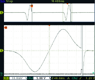
Figure 5: Induced voltage at the input stage of the driver circuit, due to the magnet in the pendulum approaching, passing over, and then receding from the sense coil. Upper trace (1) shows a complete cycle of two passages. Lower zoomed trace shows how on the trailing end of the sense pulse (1) the drive pulse (2) causes a large bipolar induced pulse in the sense coil. Screen capture was from a TDS 3032B oscilloscope.

The concentric sense and drive coils were supported by a small aluminum platform that sat on the main table, supported by three brass screws with knurled heads. These were used to level the coils: imperfect leveling caused the induced signal from the pendulum, described below, to be asymmetric. The clearance between the bottom of the pendulum and the top of the coils was 6$\pm$1 mm.

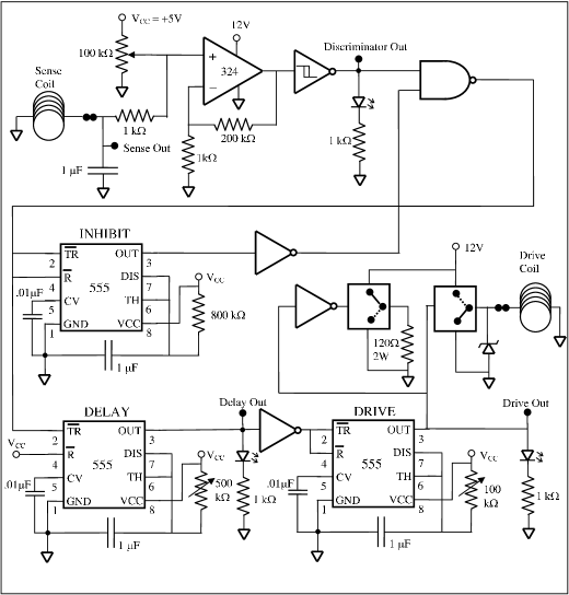
Figure 6: Circuit diagram of the pendulum driver. The op-amp (LM324) and solid-state relays (Crydom CMX60D10) are supplied by +12V, while all other components used $V_{CC}=+5$V. Unlabeled circuit elements use standard TTL chips. The “Out” connections are for monitoring the circuit on an oscilloscope.

The sense coil acted to detect the induced EMF of the swinging pendulum via Faraday induction. The typical waveform is shown in Fig. 5, showing that the approaching coil induced a negative voltage that peaked at about $V_{-}=-34$ mV, as viewed across $1M\Omega$ input impedance on an oscilloscope. When the pendulum was centered over the coil, the voltage crossed upwards through zero, followed by a positive excursion of inverted shape and the same magnitude $V_{+}$ as the negative part. The peak magnitudes of the waveform, V_±, depended on the speed of the pendulum (and hence the amplitude of the swing), as well as the distance between the pendulum magnet and the coil. Monitoring V_± over time was a sensitive way to detect small changes in the pendulum’s amplitude and/or length.

The pendulum driver circuit developed for this study is shown in Fig. 6, and operated as follows. The initial signal from the coil was filtered with a 1 $\mu$F capacitor that reduced RF noise to less than one millivolt. An op-amp circuit of type LM324N level-shifted and amplified the signal by a factor of 200. This signal was the input to a SN7414N Schmitt trigger that switched at 0.9 and 1.7 Volts. In effect, this was a discriminator with a TTL output “trigger” pulse when the induced voltage went more negative than $-20$ mV; the trigger stayed high until the trailing end of the sense-coil signal shown in Fig. 5 fell. A NAND gate output was used to trigger two 555 timers called DELAY and INHIBIT; the second input of the NAND was an inhibit signal that ensured that the DELAY timer was not restarted by the off-scale pulse induced by activation of the drive coil. The DELAY timer set the interval between the approach of the pendulum and the drive pulse in the second coil; it was adjustable in the range from near zero to several hundred milliseconds. The INHIBIT timer duration was set to be longer than the maximum possible delay plus drive times. The output of the INHIBIT timer was fed via an inverter back to the NAND, so the drive pulse could not re-fire the delay timer. The output of the DELAY timer was passed via an inverter to the input of the third 555 timer called DRIVE. This timer was adjustable over a range of several tens of microseconds, and was used to set the duration of the current through the drive coil. The output of the DRIVE timer was used to control two high-current MOSFET relays that switched current to and from the drive coil. The circuit was designed to maintain a substantial current draw from the commercial 12V switching power supply at all times, hence the dual opposite-acting relays. A Zener diode across the drive coil prevented back-emf from damaging the relay and power supply during switching. The very brief drive current was estimated to be 7.5 Amps. The circuit was constructed using the wire-wrap method and housed with its power supply in a small box. External connections were made using LEMO-style coaxial connectors, as seen in Fig. 4.

V Results

The pendulum described in the preceding section was used to determine the accuracy to the model that lead to Eq (19). The prediction that the Foucault precession rate should be unaffected by the transverse size of the elliptical motion is to be confirmed.

The measured pendulum parameters were $T=3.44\pm 0.01$sec, and $a=16.2\pm 0.2$cm. The free decay period was determined by making an exponential fit to amplitude-vs.-time data, leading to $\tau=29.7\pm 0.5$min. From these values we computed $L=2.938\pm 0.009$m, $\alpha=0.0551\pm 0.0007$, and $Q=1628\pm 28$. Solving Eq (19) numerically leads from these values to $\delta=0.319\pm 0.006$. This value in turn can be converted using Eq (9) to an expected drive time $t_{d}=178\pm 3$ms. On the other hand, the actual value of $t_{d}$ was adjusted such that a steady Foucault precession, as shown below, was observed. The direct measurement of this time using an oscilloscope gave $t_{d}=180\pm 2$ms. Thus, the model expectation as given in Eq (19) is found to be in excellent agreement with experiment with about 1% precision.

Figure 7 shows the result of a set of measurements of the precession rate spanning several days. The abscissa angles were measured from an origin arbitrarily picked to point north, with positive azimuthal angles to the counterclockwise side, as seen from above. Red circular data points are for counterclockwise and blue squares are for clockwise ellipsoidal excursions in the pendulum’s motion. Green diamond points are for readings with no measurable sense, i.e. for $b\simeq 0$. At the latitude of $\theta_{latitude}=40^{{\rm o}}26^{\prime}26"$ (Pittsburgh, Pennsylvania), the expected Foucault precession rate in one sidereal day is

$$\Omega_{F}=-\frac{2\pi}{23.935{\rm\;hours}}\sin\theta=-0.1703/{\rm hr}\to-{\rm 9.757}^{{\rm o}}/{\rm hr},$$ (26)

and this is shown as the blue bar. The vertical error bars on the points represent the estimated random measurement errors, and these were dominated by a $\pm 1/2$ degree precision of the angle measurements. The horizontal error bars represent the span of angles over which the rate was measured, with a typical span being ten degrees. The scatter of the data points clearly clusters around the expected rate, with no trend in angle or sense of ellipsoidal motion. The simple average of the measured points gives $\Omega_{F}=-9.85\pm.15$, where the given uncertainty is the error on the mean, not the standard deviation, and this is the red-dotted band shown in the figure. The weighted mean of the data gives $\Omega_{F}=-9.69\pm.09$, which is in very good agreement with the simple average, and both are in excellent agreement with the expectation of Eq (26). We prefer the former uncertainty because the wide scatter of the data points suggests that perhaps there are some small systematic effects that are not captured using the weighted mean’s uncertainty. Hence the former uncertainty is a better estimate of the true uncertainty of the result. The main candidate for a poorly-controlled systematic effect is the temperature-related changes in the length of the pendulum. Even at the sub-millimeter level, these affected the strength of the magnetic kick the pendulum received, and hence affected the value of $\alpha$, which in turn could affect control of the precession rate. We fine-tuned the length of the pendulum with shims, as needed, to minimize this effect, but the compensation was not perfect, and this probably led to some loss of reproducibility. Nevertheless, we have found the expected Foucault precession rate with an angle-integrated precision of 1.5%.

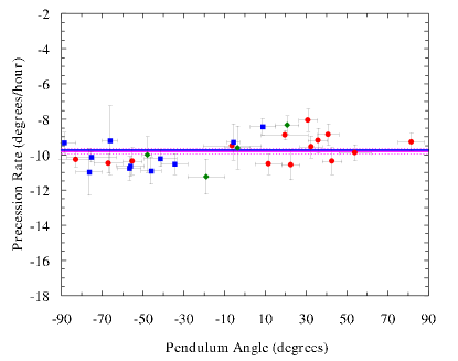
Figure 7: Precession rate as a function of azimuthal angle of the pendulum. Red circles are for counterclockwise, while blue squares are for clockwise ellipsoidal perturbation. Green diamond points were for measurements with no discernible elliptical motion. The expected rate is shown as the thick blue line. The measured average precession rate (solid) and its uncertainty band (dotted) are shown as red lines.

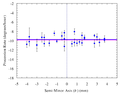
Figure 8: Precession rate as a function of the size of the semi-minor axis b of elliptical motion. Positive values of b are for counterclockwise ellipses, negative values for clockwise ellipses. The horizontal lines are the same as in the previous figure.

As discussed in connection with Eq (III), if $t_{d}$ is correctly chosen, the rate of precession in this pendulum should not depend on the size of the semi-minor axis, b. We could not control b since it depended on the small asymmetries of the fiber itself and any other perturbations of the pendulum’s motion. Of course it was damped by the effect of eddy current braking against the damping ring, but there was always some irreducible amount of ellipsoidal motion to contend with. We assign clockwise motion to have negative b values and counterclockwise motion to have positive b values. Figure 8 shows our measured precession rates, the same data set as in the previous figure, as a function of b. The size of b was measured by watching the pendulum pass over a ruler placed under the pendulum, and the precision of doing this was no better than $\pm 1$mm. We plot the points at the mean value of the ellipse size during the measurement interval. It is clear from the figure that there is no correlation between the two variables, thus proving the claim that they are in fact independent when the pendulum is properly arranged. The Foucault precession was clockwise in this northern-hemisphere setup, i.e. toward decreasing angles. Note that even when the pendulum was moving in a counterclockwise ellipse (positive values of b) that would normally precess in a counterclockwise direction, the action of the driver was such that the clockwise Foucault precession rate was unaffected. This again shows how our method nullifies the unwanted intrinsic precession.

As further evidence that our method succeeds in controlling the motion of the pendulum, we intentionally reduced the value of the driving time by $\approx 20\%$, so that the transverse kick given by $F_{\bot}$was larger than optimal. This means that any ellipsoidal precession was overcompensated by the drive system, resulting in forced precession in the opposite sense to what free oscillation would produce. Figure 9 shows the precession rate as a function of angle for $t_{d}=147\pm 1$ msec. There is, in this new situation, substantial systematic deviation from the expected rate as a function of azimuthal angle. The angle-integrated average rate is now $\Omega_{F}=-9.53\pm.57$, which is still in agreement with the expected Foucault rate, but now with a much wider error band, as shown. One also sees the propensity for clockwise ellipsoidal motion (blue squares) to decrease the magnitude of the precession rate, while counterclockwise motion (red circles) increases the magnitude of the precession rate. This is as expected in our mathematical model. There are again some cases of irreproducibility of the data points at a given angle. We believe this is the result of occasional shimming of the pendulum’s length during a multi-day run; it leads to uncontrolled small variations in the performance of the system.

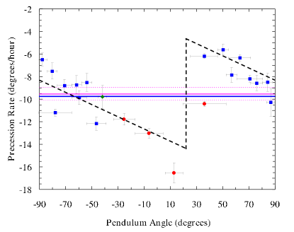
Figure 9: Precession rate as a function of azimuthal angle of the pendulum when the driving time $t_{d}$ is reduced by $\approx 20\%$ from the ideal value. As in Fig. 7, red circles are for counterclockwise, while blue squares are for clockwise ellipsoidal motion. Green diamond points were for measurements with no discernible elliptical motion. The expected rate is shown as the thick blue line. The measured average precession rate (solid) and its uncertainty band (dotted) are shown as red lines. The heavy black dashed line is a guide to the eye, as discussed in the text.

The heavy black dashed line in Fig. 9 is a guide to the eye to illustrate what happens when the ellipsoidal precession is not perfectly canceled. There is a preferred axis near $-67^{o}$, where the measured rate crosses the Foucault rate, because here the non-central forces present in the system happen to vanish. For more negative azimuthal angles (which then wrap to the positive side of the diagram) the precession rate is slower. This is because the unwanted forces act to cause clockwise ellipsoidal motion, but the drive system is overcompensating and adding a component of counterclockwise precession. At about $+23^{o}$, which is $90^{o}$ away from the preferred axis, there is a tipping point where the non-central forces act to push the pendulum in the other direction, counterclockwise. But here the overcompensating drive system makes the pendulum precess more quickly clockwise. We do not claim that the departure from the Foucault rate is strictly linear, as shown, only that the trends are consistent with our understanding of the physical process.

Finally, in Fig. 10 we show the effect of reducing the drive time $t_{d}$ by $\approx 20\%$ on the relationship between precession rate $\Omega$ and the semi-minor axis b. One sees clearly a correlation between them, whereas in Fig. 8 there was no correlation. For positive values of b (counterclockwise ellipses), the precession rate has increased magnitude since the overcompensating drive system “adds” to the Foucault rate. For negative $b$ values (clockwise ellipses) the precession rate is decreased in magnitude since the overcompensating drive system “subtracts” from the Foucault rate. Thus, we have shown that when deviating from the prediction of Eq (19) for the correct drive distance, and therefore the correct drive time, the pendulum shows marked departure from the constant Foucault precession rate that is expected.

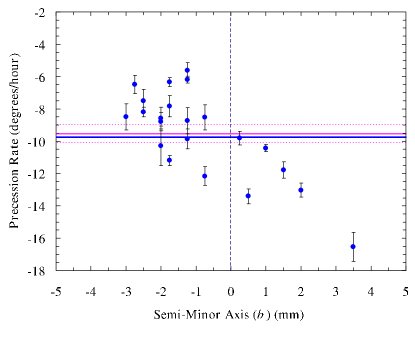
Figure 10: Precession rate as a function of the size of the semi-minor axis b when the driving time $t_{d}$ is reduced by $\approx 20\%$ from the predicted value. Positive values of b are for counterclockwise ellipses, negative values for clockwise ellipses. This figure is to be compared with Fig. 8.

VI Further Discussion and Conclusions

In the previous work of Crane cra2 , he recognized the importance of nullifying the intrinsic precession that remains after damping as well as possible. However, he used a “push-pull” drive system to mitigate problems of alignment of the coils with the pendulum. This led him to introduce a carefully-placed fixed permanent magnet at the origin to provide the desired stopping of intrinsic precession. No quantitative understanding of how to predict the placement of this magnet was offered. It seems to us that his very delicate ad hoc adjustment of this auxiliary magnet is difficult, and, as we have shown, not necessary. Our method is simpler and more direct, in that it does not require this additional magnet. Alignment of the driving and sense coils was not found to be a problem, and the results were not sensitive to the alignment at the level of about a millimeter. This was because the method we have introduced is in a sense self-correcting: if the drive coil causes some small amount of ellipsoidal motion, the very action of the method prevents this motion from causing unwanted precession. The work of Mastner et al.  mas made note of the benefits of a “push only” driving force, but they did not offer the quantitative explanation as to how and why it worked. They built a traditional, very long, very massive pendulum, taking great care to minimize asymmetries.

In conclusion, we have demonstrated the workings of a “short” Foucault pendulum that was designed on a quantitative basis to avoid the unwanted precession due to ellipsoidal motion. The design formula we have derived, Eq (19), was shown to agree with measured values in our setup. We have shown that a driving mechanism that pushes, not pulls, the pendulum is the key to canceling the intrinsic precession for all values of the semi-minor axis of the ellipse. Our driver system used Faraday induction and magnetic repulsion to control the pendulum, using a circuit based on simple op-amp, logic, and timer chips. Eddy current damping was used to reduce the ellipse size, but active compensation did the rest. The design is immune to small non-central forces that are difficult to control in a short pendulum. We plan to further test this method on even shorter pendula, since there is no lower limit at which the model given here should apply.

VII Acknowledgments

We thank Mr. Gary Wilkin for his expert help in the machine shop. We thank Mr. Michael Vahey for construction of the pendulum driver, and we thank Mr. Chen Ling for help with exploratory initial trials in construction of a Foucault pendulum.

References

- (1) M. L. Foucault, “Démonstration physique du mouvement de rotation de la terre au moyen du pendule” Comptes Rendus Acad. Sci. 32, 135-138 (1851).
- (2) M. G. Olsson, “The precessing spherical pendulum,” Am. J. Phys. 46, 1118-1119 (1978).
- (3) M. G. Olsson, “Spherical pendulum revisited,” Am. J. Phys. 49, 531-534 (1981).
- (4) A. B. Pippard, “The parametrically maintained Foucault pendulum and its perturbations,” Proc. R. Soc. Lond. A420, 81-91 (1988).
- (5) J. Synge and B. Griffith, Principles of Mechanics (McGraw Hill, 1959), 3rd ed., pp 335-342.
- (6) M. Charron, “Sur un perfectionnement du pendule de Foucault et sur l’entretien des oscillations,” Comptes Rendus Acad. Sci. 192, 208-210 (1931).
- (7) See for example C.F. Moppert and W. J. Bonwick, “The New Foucault Pendulum at Monash University”, Q. Jl. R. Astr. Soc. 21, 108-118 (1980), and references therein. Also Haym Kruglak et al, “A short Foucault pendulum for a hallway exhibit”, Am. J. Phys. 46, 438-440 (1978).
- (8) H. Richard Crane, “The Foucault Pendulum as a murder weapon and a physicist’s delight”, Phys. Teach. 264-269 (May 1990).
- (9) H. Richard Crane, “Foucault pendulum “wall clock””, Am. J. Phys. 63, 33-39 (1995); “Short Foucault Pendulum: A Way to Eliminate the Precession due to Ellipticity”, Am. J. Phys. 49, 1004-1006 (1981).
- (10) G. Mastner et al, “Foucault pendulum with eddy-current damping of the elliptical motion”, Rev. Sci. Inst. 55, 1533-1538 (1984).
- (11) Joseph Priest and Michael Pechan, “The driving mechanism for a Foucault pendulum (revisited)”, Am. J. Phys. 76, 188-188 (2008).